TL;DR#
Despite rapid advances in AI benchmarks, their real-world implications remain unclear. This paper addresses this by introducing the 50%-task-completion time horizon: the time humans take to complete tasks AI models can achieve with 50% success. Researchers timed humans on tasks from RE-Bench, HCAST, and novel shorter tasks to benchmark AI performance. This metric allows for a more intuitive comparison of AI capabilities to human capabilities.
The paper evaluates 13 frontier AI models from 2019 to 2025, finding the time horizon has been doubling every seven months. This exponential growth is attributed to better reliability, adaptability, logical reasoning, and tool use. The study also acknowledges limitations, such as external validity and potential impact on dangerous capabilities, predicting AI may automate many software tasks within five years.
Key Takeaways#
Why does it matter?#
This paper is important for researchers by providing a quantifiable metric to track and forecast AI capabilities, aiding in responsible AI governance and risk mitigation. It opens avenues for studying factors influencing AI progress and its impact on dangerous capabilities. Understanding and forecasting AI capabilities are crucial for policymakers, AI developers, and safety researchers alike.
Visual Insights#

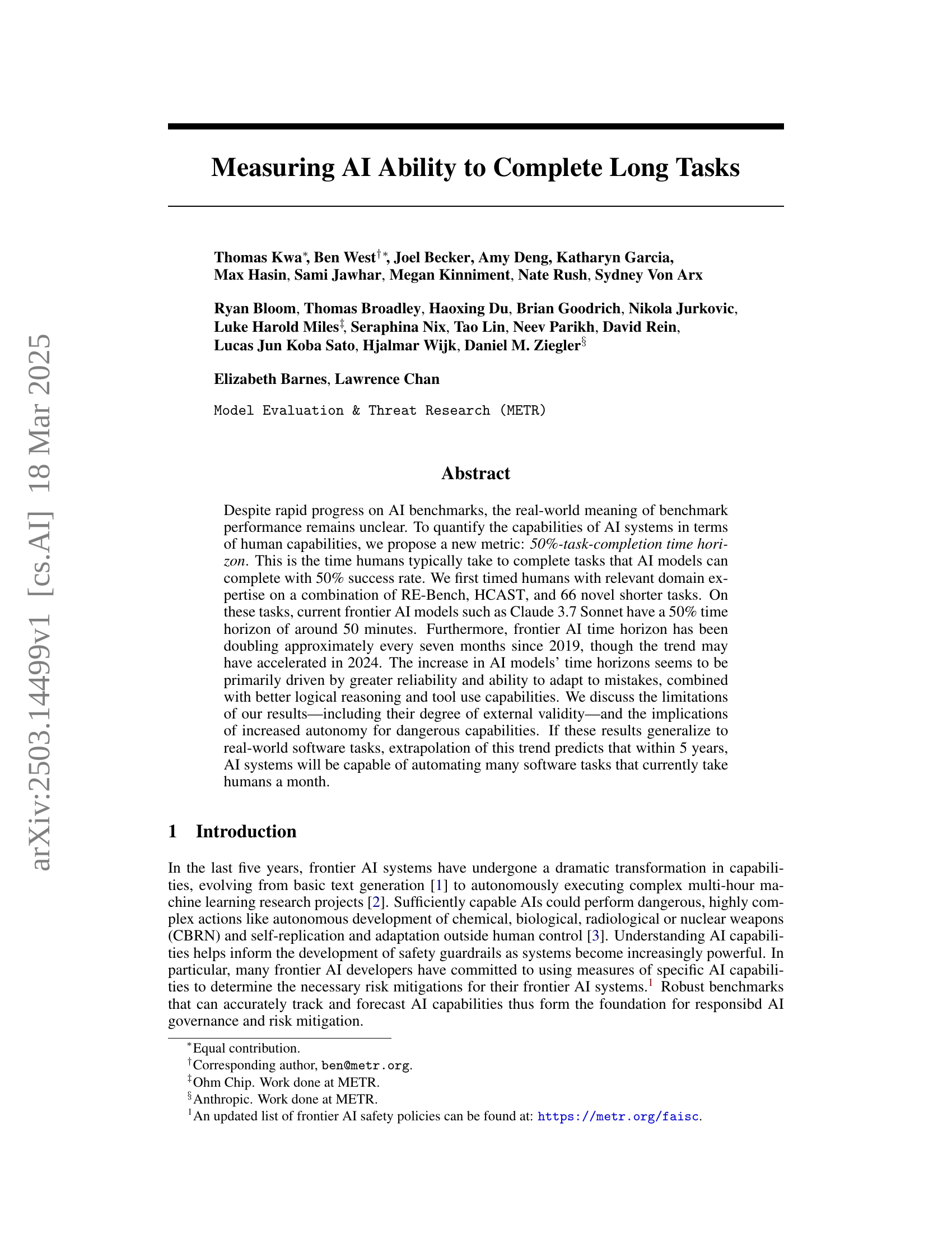
🔼 This figure displays the exponential growth of AI capabilities over the past six years. It shows the length of time it takes human professionals to complete tasks that AI models can perform with 50% reliability (the 50% task completion time horizon). The data indicates that this time horizon has doubled roughly every seven months since 2019. The shaded area represents the 95% confidence interval, calculated using a robust statistical method called hierarchical bootstrapping to account for variations in task difficulty and model performance. Even with a significant margin of error in the absolute measurements, the observed trend strongly suggests that within the next decade, AI systems will be capable of completing a substantial portion of software tasks that currently take humans days or weeks to finish.
read the caption
Figure 1: The length of tasks (measured by how long they take human professionals) that generalist autonomous frontier model agents can complete with 50% reliability has been doubling approximately every 7 months for the last 6 years (Section 4). The shaded region represents 95% CI calculated by hierarchical bootstrap over task families, tasks, and task attempts. Even if the absolute measurements are off by a factor of 10, the trend predicts that in under a decade we will see AI agents that can independently complete a large fraction of software tasks that currently take humans days or weeks(Section 7).
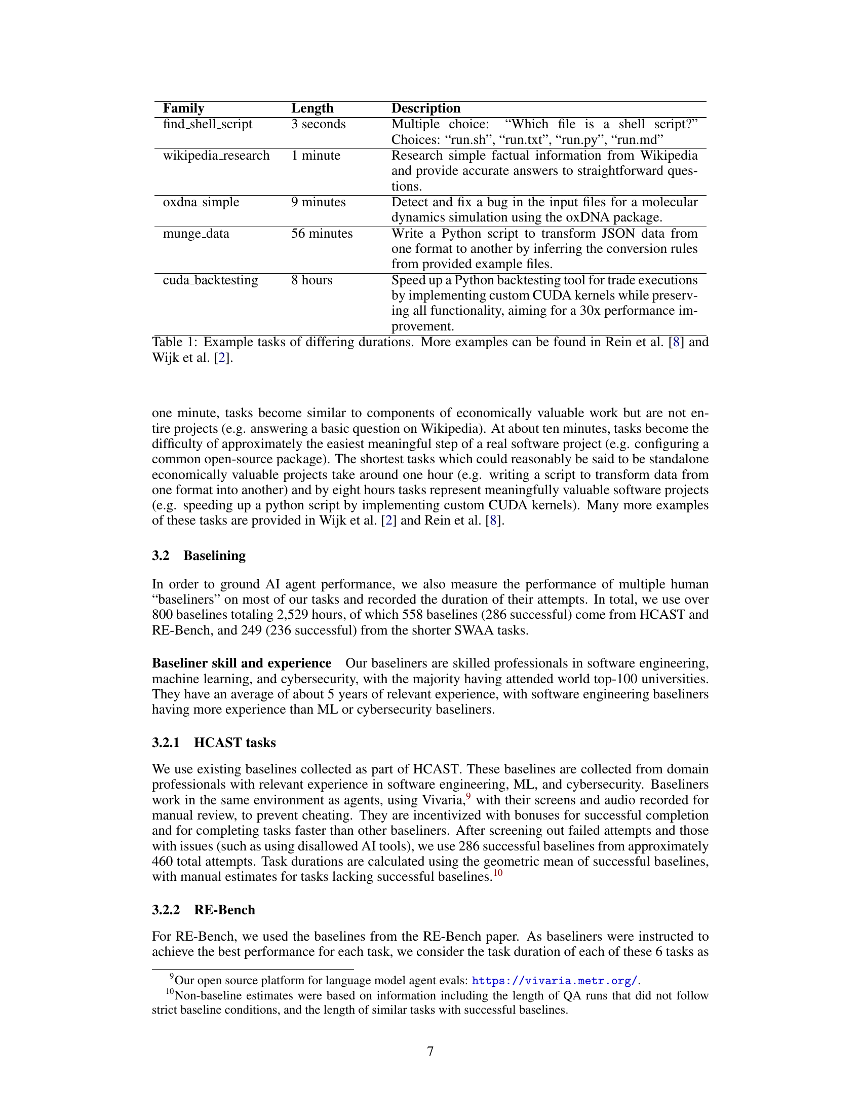
| Family | Length | Description |
|---|---|---|
| find_shell_script | 3 seconds | Multiple choice: “Which file is a shell script?” Choices: “run.sh”, “run.txt”, “run.py”, “run.md” |
| wikipedia_research | 1 minute | Research simple factual information from Wikipedia and provide accurate answers to straightforward questions. |
| oxdna_simple | 9 minutes | Detect and fix a bug in the input files for a molecular dynamics simulation using the oxDNA package. |
| munge_data | 56 minutes | Write a Python script to transform JSON data from one format to another by inferring the conversion rules from provided example files. |
| cuda_backtesting | 8 hours | Speed up a Python backtesting tool for trade executions by implementing custom CUDA kernels while preserving all functionality, aiming for a 30x performance improvement. |
🔼 This table presents example tasks from the study, categorized by the time it takes a human expert to complete them. It showcases the diversity of tasks used in the research, ranging from simple, short tasks (seconds) to complex, lengthy tasks (hours). The purpose is to illustrate the range of complexity the AI models were evaluated on, and to provide a sense of the scale of tasks involved. Further examples of tasks can be found in the cited papers.
read the caption
Table 1: Example tasks of differing durations. More examples can be found in Rein et al. [8] and Wijk et al. [2].
In-depth insights#
AI Task Autonomy#
The progression of AI task autonomy, highlighted in the document, signifies a critical shift towards systems capable of independently executing complex, real-world tasks. The focus on longer task completion time horizons as a metric acknowledges the importance of AI’s ability to sustain performance over extended periods, mirroring human capabilities. Improving AI’s reliability and adaptability are crucial drivers, enabling systems to handle complexities and recover from errors autonomously. Benchmarking against human baselines provides a tangible measure of AI’s progress, emphasizing practical skills in research and software engineering. Measuring the time AI can autonomously perform tasks with reasonable success, sets an intuitive, real-world standard. Emphasis on tool usage and logical reasoning underscores the multifaceted nature of AI competence. The potential for automating complex software tasks heralds a new era, demanding vigilance regarding safety and ethical implications as AI transcends current human task execution.
50% Comp. Horizon#
The research paper introduces the 50% task completion time horizon, a new metric for gauging AI capabilities by measuring the time humans take to complete tasks AI models can achieve with 50% success. This horizon is determined by timing human experts on tasks, then assessing AI models’ performance. The doubling time for the AI time horizon is about 7 months, indicating rapid progress. The 50% threshold highlights the point where AI reliably performs tasks, providing a practical measure of automation potential. This metric reflects AI’s evolving proficiency in handling diverse tasks, offering a tangible way to track progress beyond benchmark scores. External validity is key to the metric’s relevance, ensuring the trend holds for real-world software tasks. Understanding this trajectory is crucial for informing AI safety measures.
Exponential Growth#
The research indicates the exponential growth of AI capabilities, specifically in completing tasks of increasing length. This trend, measured by the time horizon of tasks AI can reliably perform, suggests a rapid advancement in AI autonomy. Extrapolating this exponential trend raises significant implications. It could lead to AI systems capable of automating complex software tasks currently requiring human expertise, potentially transforming industries. It underscores the need for careful consideration of AI safety and governance, as such exponentially improving capabilities could also pose risks if not managed responsibly.
Messiness Matters#
The research acknowledges that real-world intellectual labor involves messy details absent from benchmarks. These include under-specification, unclear feedback loops, and coordination challenges. The study addresses whether AI agents show similar improvement rates on less and more messy tasks. Tasks were rated on 16 ‘messiness’ properties to quantify this. While agents struggled more with messier tasks, performance trends remained consistent across messiness levels. The mean ‘messiness score’ among HCAST and RE-Bench tasks is found to be 3.2/16, suggesting that these tasks are not as messy as real-world scenarios, for example, ‘write a good research paper’ may score from 9/16 to 15/16.
Extrap. w/ Caution#
Extrapolating AI capabilities requires caution. While trends suggest rapid progress, projecting future performance is complex. External validity concerns arise as benchmarks might not reflect real-world tasks accurately. The AI progress which includes agency training, compute scaling, and R&D automation could alter the time horizon. Forecasting AI’s impact is sensitive to doubling rate changes rather than constant factors. Although time horizon offers an intuitive measure, it’s linked to task distributions and baseliner context. Therefore, extrapolations are uncertain and rely on continuous monitoring and careful re-evaluation.
More visual insights#
More on figures

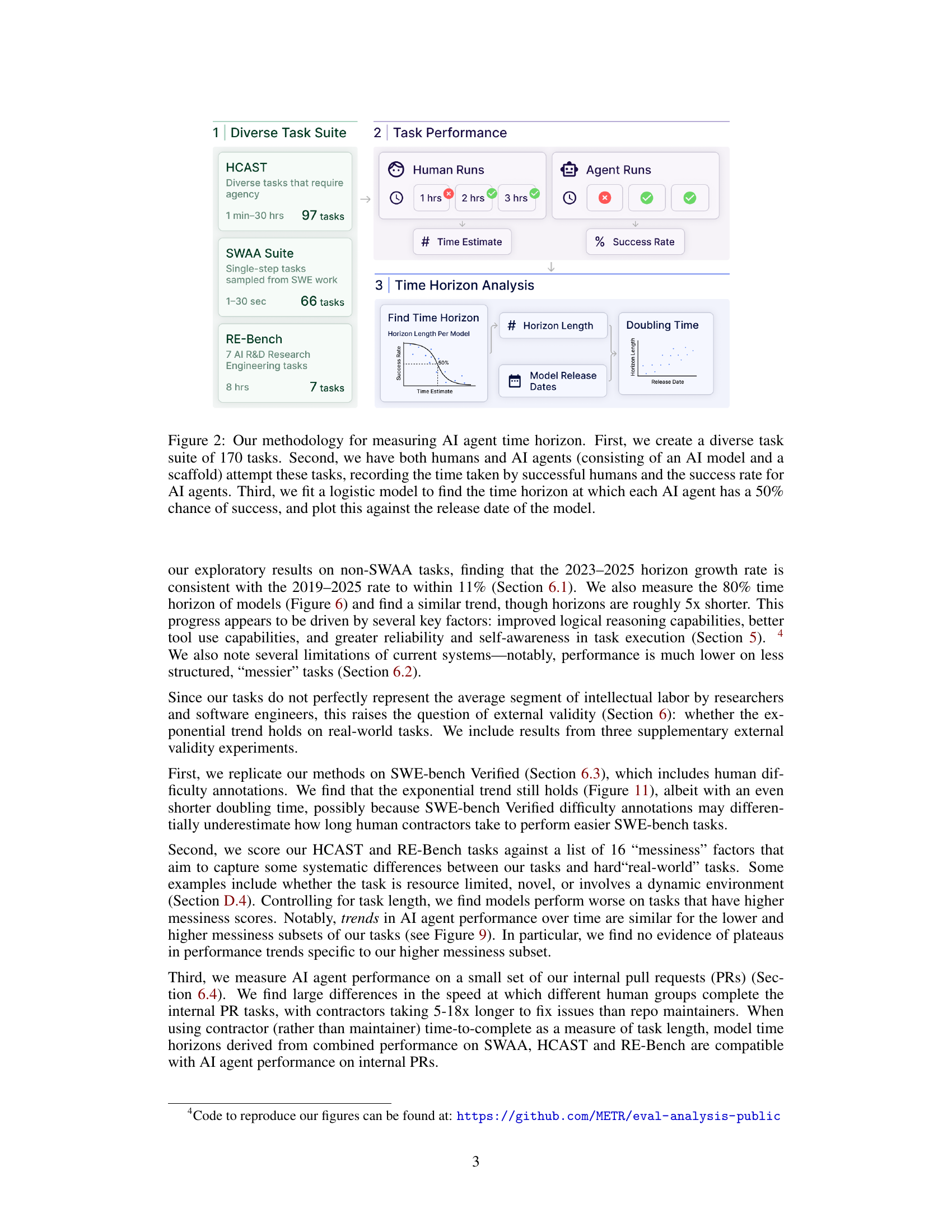
🔼 This figure illustrates the methodology used to measure AI agent time horizons. The process involves three main steps: 1) Creation of a diverse task suite (170 tasks) spanning a wide range of complexities, 2) Task completion by both humans and AI agents (AI models using scaffolds) where human completion times and AI success rates are recorded, and 3) Fitting of a logistic model to determine the time horizon (the time it takes humans to complete tasks an AI can do with a 50% success rate) for each AI model. These time horizons are then plotted against the model’s release dates.
read the caption
Figure 2: Our methodology for measuring AI agent time horizon. First, we create a diverse task suite of 170 tasks. Second, we have both humans and AI agents (consisting of an AI model and a scaffold) attempt these tasks, recording the time taken by successful humans and the success rate for AI agents. Third, we fit a logistic model to find the time horizon at which each AI agent has a 50% chance of success, and plot this against the release date of the model.

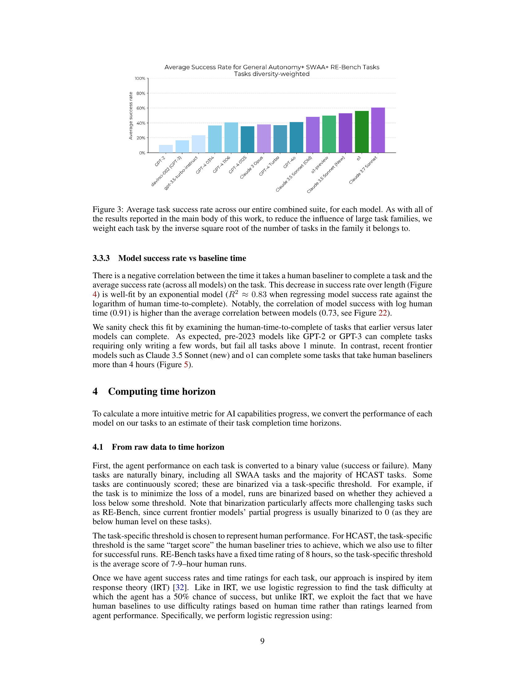
🔼 This figure displays the average success rate of various AI models on a diverse set of tasks. The tasks are categorized into families, and to avoid bias from families with many tasks, each task’s contribution to the average is weighted. The weighting scheme used is the inverse square root of the number of tasks within its family. This ensures that no single task family disproportionately affects the overall results. The graph shows a clear trend of improved performance over time as newer models achieve higher average success rates.
read the caption
Figure 3: Average task success rate across our entire combined suite, for each model. As with all of the results reported in the main body of this work, to reduce the influence of large task families, we weight each task by the inverse square root of the number of tasks in the family it belongs to.

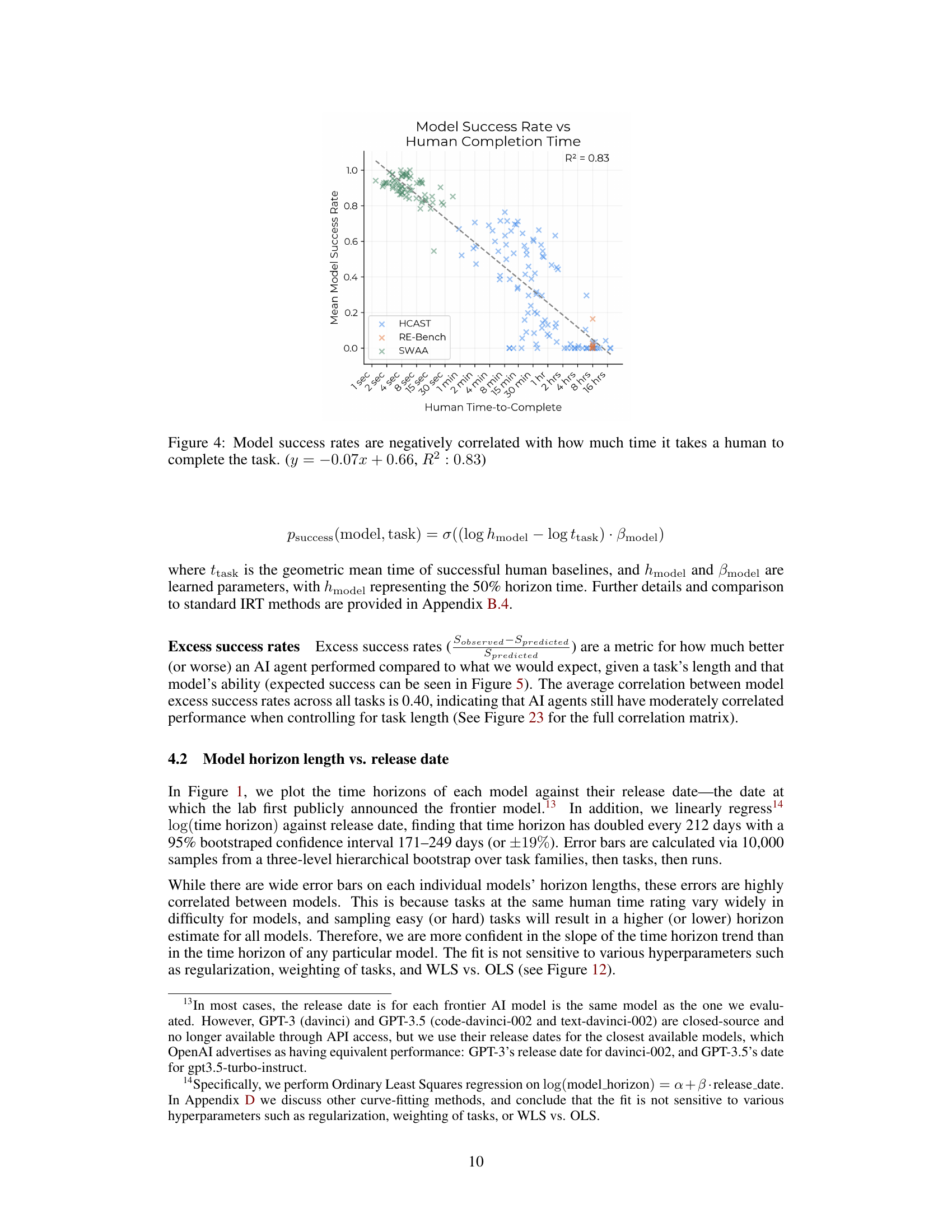
🔼 This figure shows the negative correlation between the time it takes a human expert to complete a task and the average success rate of AI models on that task. The x-axis represents the time (in minutes) it takes a human to complete the task, while the y-axis represents the AI model’s average success rate. The data points represent individual tasks, and the line represents a linear regression fit to the data. The R-squared value of 0.83 indicates a strong correlation, suggesting that tasks that are easy for humans are also easy for AI models to complete successfully, while more difficult tasks for humans are also more challenging for AI models.
read the caption
Figure 4: Model success rates are negatively correlated with how much time it takes a human to complete the task. (y=−0.07x+0.66𝑦0.07𝑥0.66y=-0.07x+0.66italic_y = - 0.07 italic_x + 0.66, R2:0.83:superscript𝑅20.83R^{2}:0.83italic_R start_POSTSUPERSCRIPT 2 end_POSTSUPERSCRIPT : 0.83)

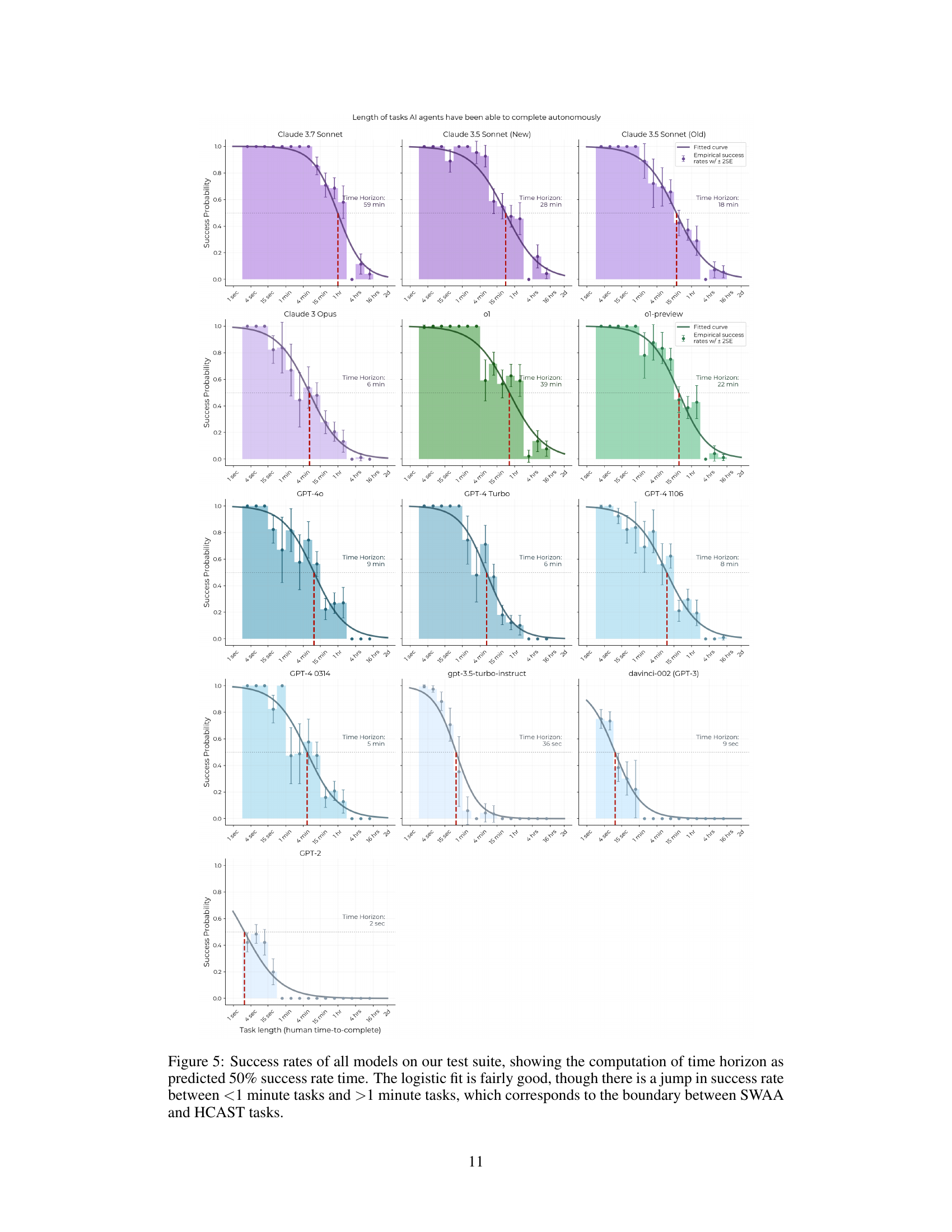
🔼 Figure 5 presents a comprehensive analysis of the success rates achieved by various AI models across a diverse range of tasks categorized by their duration. The x-axis represents the time taken for human professionals to complete the tasks, ranging from sub-second durations to several hours. The y-axis represents the success rate of each AI model on the corresponding tasks. The figure uses a logistic regression model to fit the data and graphically represent the AI model’s 50% time horizon. The 50% time horizon, shown as a vertical line intersecting the model’s curve, signifies the task duration at which the AI model achieves a 50% success rate. A notable observation is the apparent jump in success rate between tasks lasting less than one minute and tasks taking longer than one minute, reflecting the distinct nature of the shorter SWAA and longer HCAST task sets.
read the caption
Figure 5: Success rates of all models on our test suite, showing the computation of time horizon as predicted 50% success rate time. The logistic fit is fairly good, though there is a jump in success rate between <1 minute tasks and >1 minute tasks, which corresponds to the boundary between SWAA and HCAST tasks.

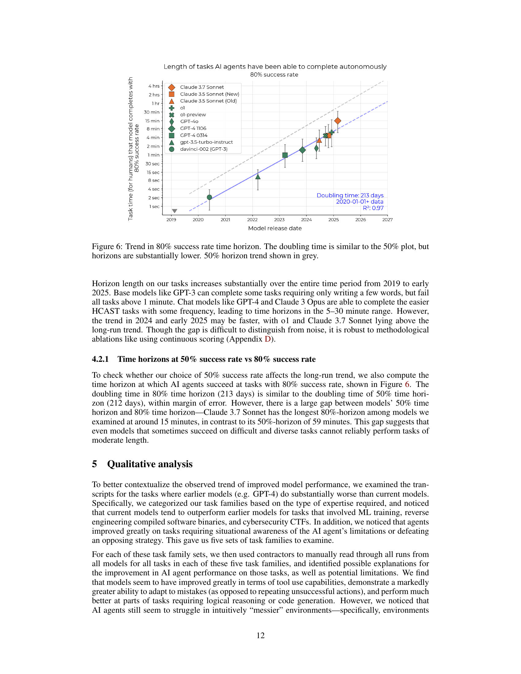
🔼 Figure 6 shows the exponential growth of AI capabilities over time, measured by the 80% task completion time horizon. This metric represents the length of tasks that AI models can complete with an 80% success rate. The figure plots this horizon length against the model’s release date. The key finding is that the 80% time horizon has been doubling approximately every seven months, a trend very similar to the 50% time horizon (shown in grey for comparison). However, the 80% time horizon consistently remains significantly shorter than the 50% time horizon, indicating that while AI models are improving rapidly, their reliability is still a factor that needs improvement before consistently handling longer tasks.
read the caption
Figure 6: Trend in 80% success rate time horizon. The doubling time is similar to the 50% plot, but horizons are substantially lower. 50% horizon trend shown in grey.

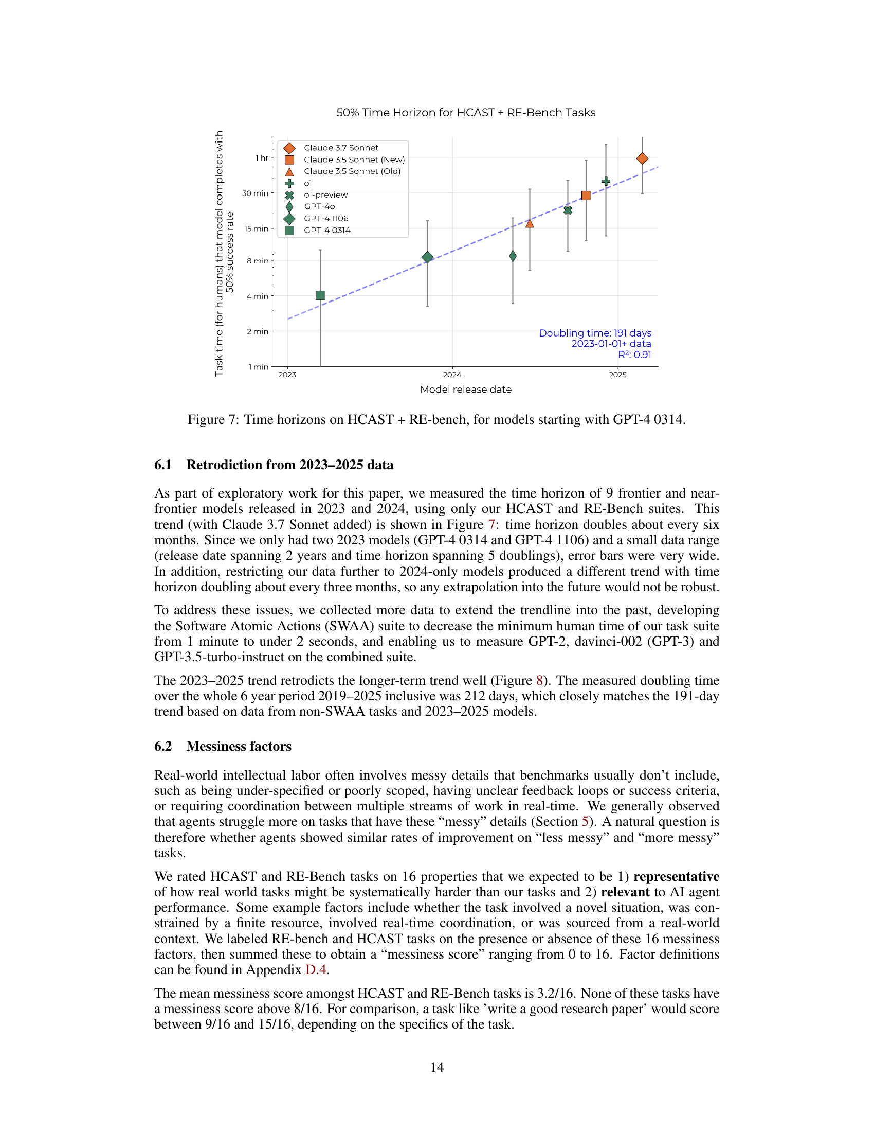
🔼 This figure shows the trend of AI model capabilities over time, specifically focusing on the time it takes for AI models to complete tasks of increasing difficulty, as measured by human completion time. The x-axis represents the release date of the AI model, and the y-axis represents the length of the task (in human time) that a model can complete with a 50% success rate (the 50% time horizon). The data used in this figure includes tasks from HCAST and RE-Bench. The model trendline shows exponential growth in AI capabilities over the observed period. Starting from GPT-4 0314, it shows how the model’s 50% time horizon has grown exponentially.
read the caption
Figure 7: Time horizons on HCAST + RE-bench, for models starting with GPT-4 0314.

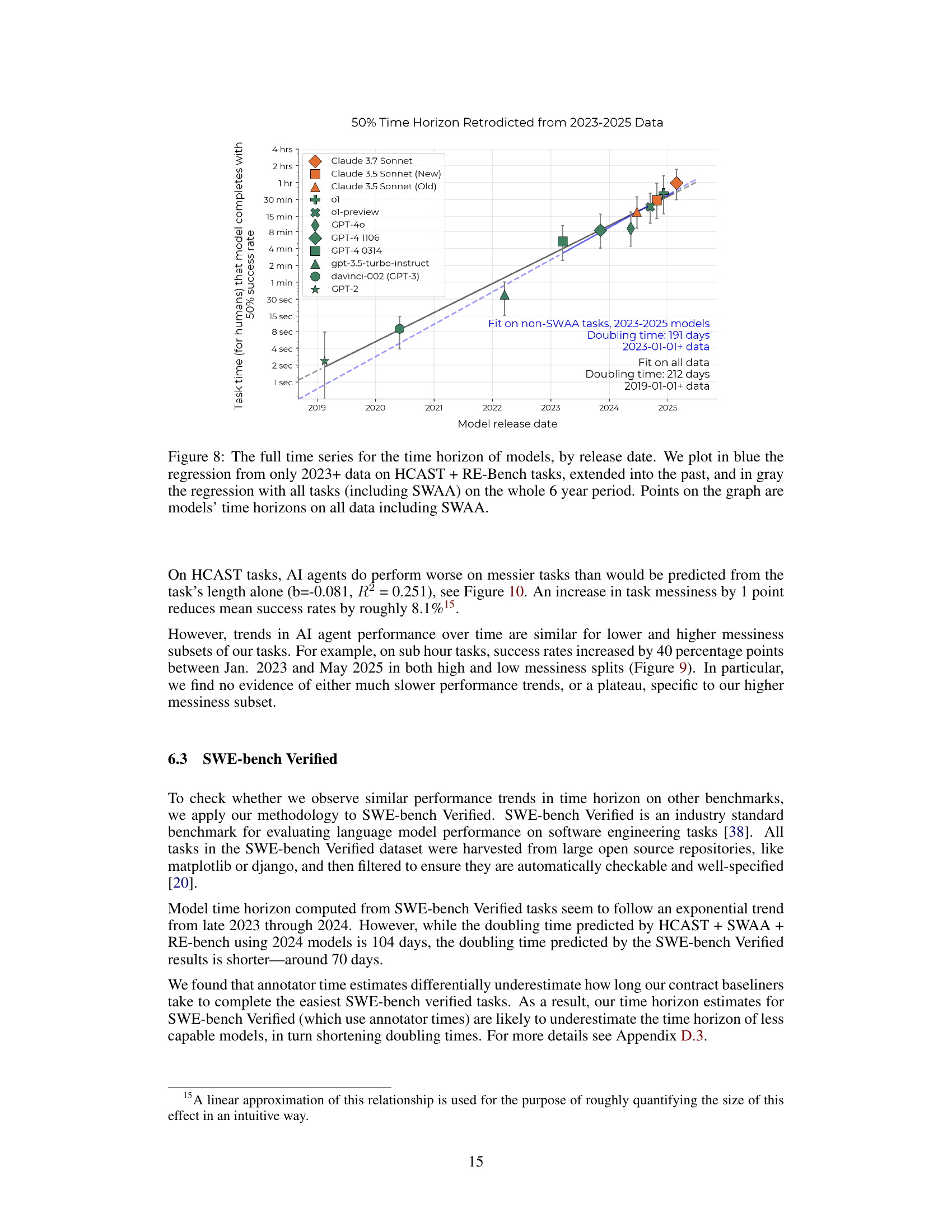
🔼 Figure 8 presents a comprehensive analysis of the relationship between AI model release dates and their corresponding 50% task completion time horizons. The graph displays two regression lines: one (blue) calculated from data on HCAST and RE-Bench tasks from 2023 onward, extrapolated back to 2019; and another (gray) computed using all task data (including SWAA) across the entire six-year period. Data points represent the actual 50% task completion time horizons for each model, calculated using the complete dataset. This dual-regression approach allows for a comparison of the growth trend observed in more recent models against the overall trend observed throughout the six-year period.
read the caption
Figure 8: The full time series for the time horizon of models, by release date. We plot in blue the regression from only 2023+ data on HCAST + RE-Bench tasks, extended into the past, and in gray the regression with all tasks (including SWAA) on the whole 6 year period. Points on the graph are models’ time horizons on all data including SWAA.

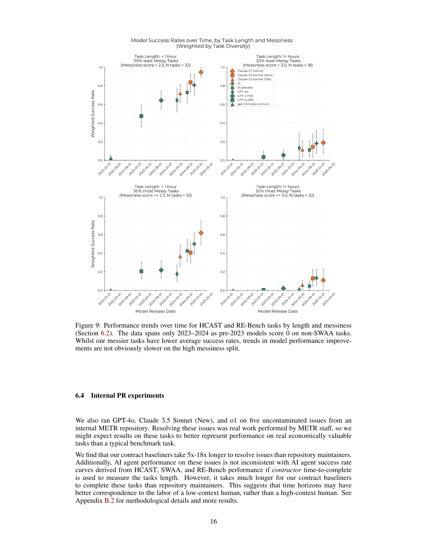
🔼 Figure 9 presents a detailed analysis of how the performance of AI models changes over time on tasks categorized by length (less than 1 hour vs. 1 hour or more) and messiness (a measure of task complexity, considering factors like clarity of instructions and resource limitations). The analysis focuses on data from 2023-2024 because pre-2023 models performed poorly on the more complex tasks. The figure displays the weighted average success rate of multiple models across the two task lengths and messiness levels. While messier tasks show lower average success rates, the graph indicates that the rate of model performance improvement is consistent across both high and low messiness levels, suggesting that the increasing capabilities of AI models are not significantly hindered by task complexity.
read the caption
Figure 9: Performance trends over time for HCAST and RE-Bench tasks by length and messiness (Section 6.2). The data spans only 2023–2024 as pre-2023 models score 0 on non-SWAA tasks. Whilst our messier tasks have lower average success rates, trends in model performance improvements are not obviously slower on the high messiness split.

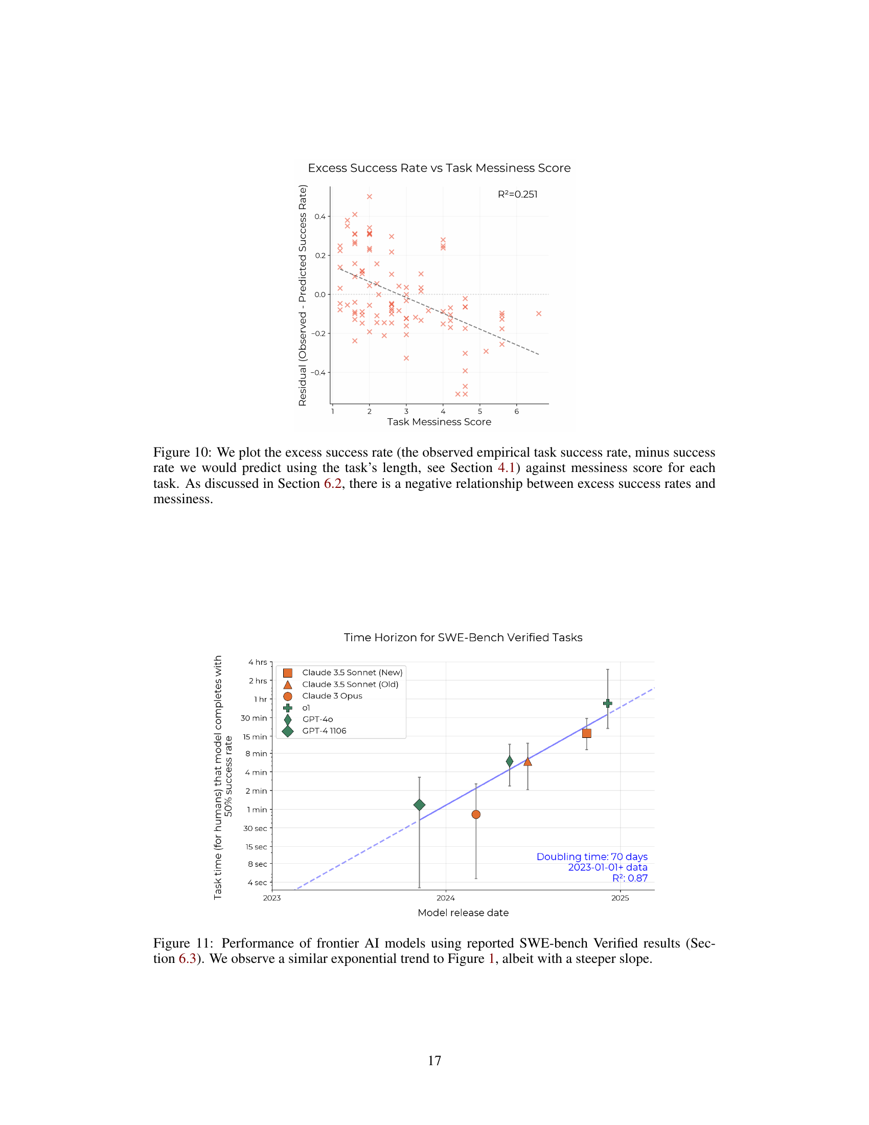
🔼 This figure illustrates the correlation between task ‘messiness’ and the performance of AI models. The x-axis represents the ‘messiness score’ of each task, indicating its complexity and real-world resemblance. The y-axis shows the ’excess success rate’, calculated as the difference between a model’s actual success rate on a task and the rate predicted based solely on the task’s length (as detailed in section 4.1). The plot reveals a negative correlation: as task messiness increases, the excess success rate of AI models decreases, suggesting that AI models struggle more with complex, less structured tasks.
read the caption
Figure 10: We plot the excess success rate (the observed empirical task success rate, minus success rate we would predict using the task’s length, see Section 4.1) against messiness score for each task. As discussed in Section 6.2, there is a negative relationship between excess success rates and messiness.

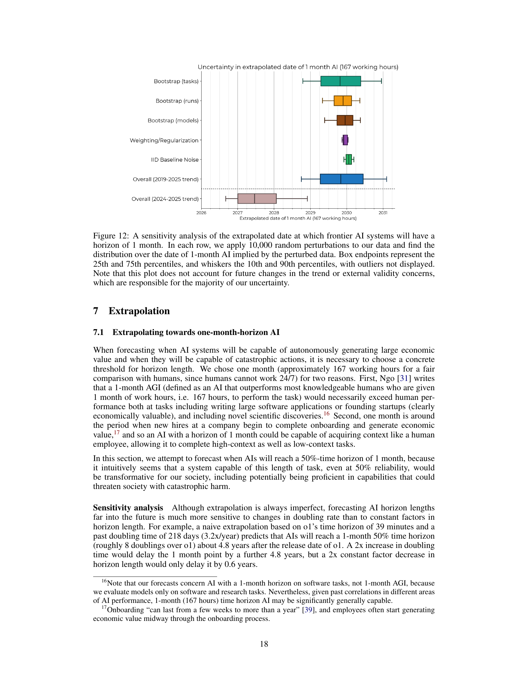
🔼 Figure 11 shows the results of evaluating the performance of several frontier AI models on the SWE-Bench Verified benchmark. The benchmark consists of software engineering tasks. This figure plots the 50% task completion time horizon of each model against its release date. This figure demonstrates an exponential trend in AI model capabilities, similar to the trend observed in Figure 1, but the doubling time is shorter, indicating a steeper improvement rate over time for these specific tasks.
read the caption
Figure 11: Performance of frontier AI models using reported SWE-bench Verified results (Section 6.3). We observe a similar exponential trend to Figure 1, albeit with a steeper slope.

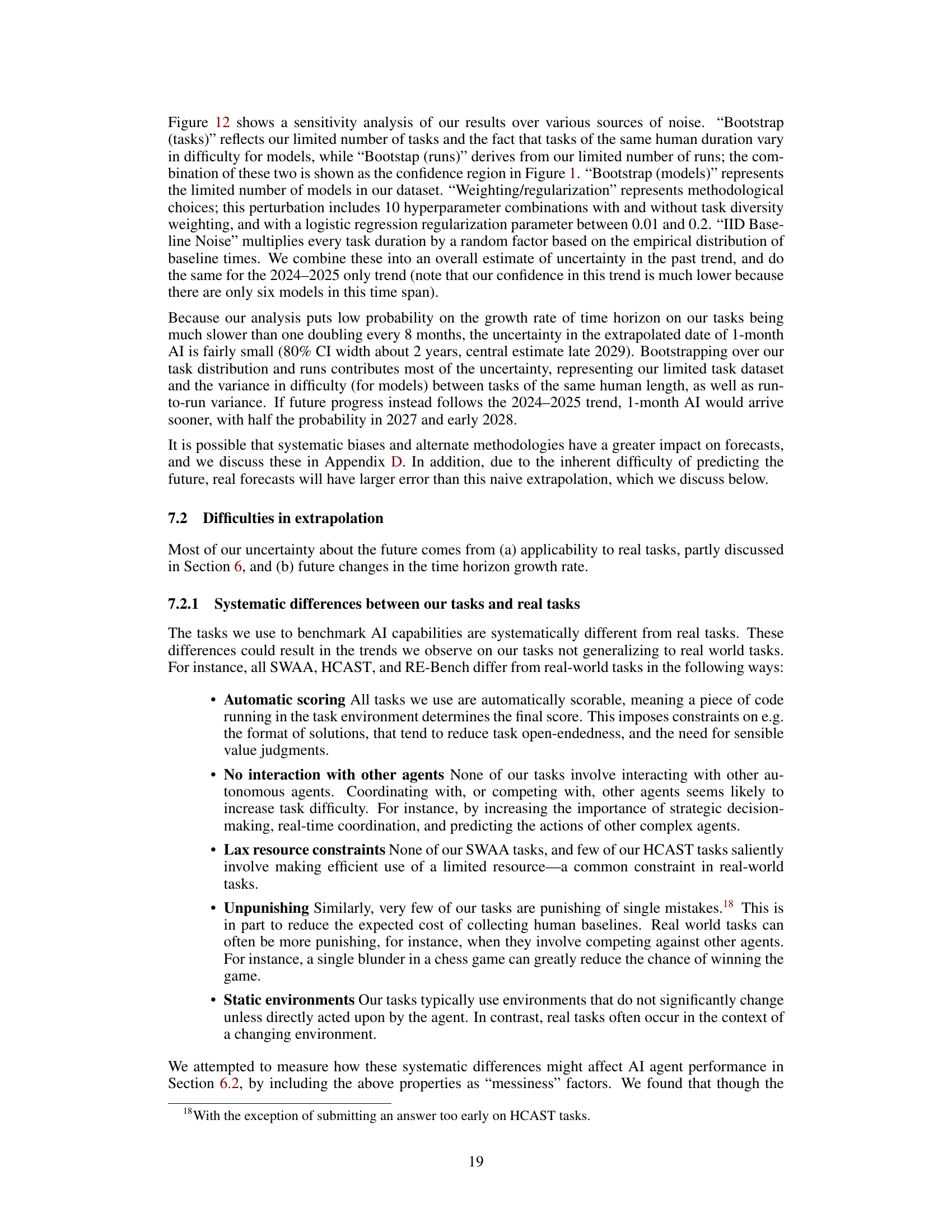
🔼 This figure presents a sensitivity analysis to determine when frontier AI systems might reach a 1-month task completion time horizon. The analysis involves introducing random variations to the data and observing the resulting changes in the projected date. The box plots display the 25th to 75th percentiles (the interquartile range), with the whiskers extending to encompass the 10th and 90th percentiles. Data points outside this range (outliers) are not shown. Importantly, the analysis acknowledges that future changes in the growth trend and external factors not considered here could significantly impact the prediction.
read the caption
Figure 12: A sensitivity analysis of the extrapolated date at which frontier AI systems will have a horizon of 1 month. In each row, we apply 10,000 random perturbations to our data and find the distribution over the date of 1-month AI implied by the perturbed data. Box endpoints represent the 25th and 75th percentiles, and whiskers the 10th and 90th percentiles, with outliers not displayed. Note that this plot does not account for future changes in the trend or external validity concerns, which are responsible for the majority of our uncertainty.

🔼 This figure shows the cost-effectiveness of using large language models (LLMs) to perform tasks compared to human experts. The y-axis represents the ratio of the cost of a successful LLM run to the cost of a human expert performing the same task. The x-axis represents the duration of the task in human time. Each point represents a single task. The plot visualizes how the cost-effectiveness of LLMs varies across tasks of different lengths.
read the caption
Figure 13: Cost of a successful run using an LLM agent as a fraction of the cost of the salary of a human expert performing the same task.

🔼 This figure is a stacked histogram showing the distribution of task difficulty across three different datasets: HCAST, RE-Bench, and SWAA. The x-axis represents the time it takes a human expert to complete the tasks, ranging from fractions of a second to many hours. The y-axis shows the number of tasks. The HCAST dataset is heavily weighted towards tasks that take more than 4 minutes to complete, while the SWAA dataset focuses on tasks in the 2-15 second range. The distribution is highly skewed with most tasks concentrated in the shorter time frames. This skew is partly due to the choice to include SWAA in order to extend the ability to measure time horizons to earlier models such as GPT-2 and GPT-3. However, the resulting gap between the SWAA and HCAST data limits the accuracy of the time horizon measurements in the intermediate range.
read the caption
Figure 14: Stacked histogram of tasks by difficulty rating. HCAST mainly includes tasks longer than 4 minutes, while we focused on tasks in the 2-second to 15-second range with SWAA in order to measure GPT-2 and GPT-3. There is a gap between the two which limits our ability to measure time horizons in this range.

🔼 This figure lists seven tasks from the RE-Bench benchmark. Each task description includes the environment in which the task was performed, a brief description of the task, and the scoring metric used. The table provides a concise overview of the complexities and variety of tasks within the benchmark, highlighting the range of skills and knowledge required for successful AI performance.
read the caption
Figure 15: The 7 original RE-Bench tasks.

🔼 Figure 16 shows the performance of human baseliners on the tasks. It presents the success rate of human baseliners across different task lengths, along with a fitted logistic curve to estimate the time horizon. The time horizon represents the task length at which human baseliners achieve a 50% success rate. Importantly, the caption notes that this time horizon is not directly comparable to the time horizon calculated for ML models (as explained in Section B.1.1), due to methodological differences in how the time horizons are calculated and the inclusion of factors such as human attention spans that don’t affect ML models.
read the caption
Figure 16: Success rates and time horizon of human baseliners. Note that the time horizon is not directly comparable to the time horizon of ML models (see Section B.1.1)

🔼 This figure compares three different curve fits (linear, hyperbolic, and exponential) to model the growth of AI agent time horizons since 2019. The exponential fit shows a strong correlation and provides a doubling time, while the linear and hyperbolic fits show significantly weaker correlations. The choice of an exponential fit in the main analysis is justified by its superior fit and fewer parameters, reducing the risk of overfitting.
read the caption
Figure 17: Linear, hyperbolic, and exponential fits for model time horizon since 2019.

🔼 Figure 18 shows the time horizon calculated using continuous scoring instead of binarizing the task success. The continuous scoring method is believed to better capture the true capabilities of the models, especially on the longer, more complex RE-Bench tasks (8 hours). However, this approach may inflate the time horizon, particularly for newer models, because achieving an average success rate of 50% is generally less challenging than consistently matching human performance 50% of the time. This effect is amplified for longer tasks that are more frequently assessed using continuous scores. The figure shows that the time horizon for AI models is increasing exponentially.
read the caption
Figure 18: Time horizon with continuous (non-binarized) scoring. Claude 3.7 Sonnet has a 50% time horizon of nearly 2 hours. We think this methodology captures more signal from 8-hour RE-Bench tasks, but overstates the time horizon of recent models, since it is easier to achieve an average score of 0.5 on most tasks than to match human performance 50% of the time. The slope is also likely an overestimate, because longer tasks tend to be continuously scored.

🔼 This figure displays two exponential regression fits modeling the growth of AI capabilities over time, specifically the 50% time horizon. The x-axis represents the model’s release date. The y-axis shows the length of time (in hours) it takes a human professional to complete a task that the AI model can complete with 50% success. The gray line represents the fit using data from 2019 to 2025. The blue line shows the fit using only data from 2024 and 2025. This visual comparison demonstrates that while a general trend of exponential growth is consistent across the entire period, a steeper growth rate may have been observed in the more recent years.
read the caption
Figure 19: 2024–2025 and 2019–2025 exponential fits for 50% time horizon.

🔼 Figure 20 is a scatter plot that examines the relationship between task messiness and the time it takes for a human to complete the task. The x-axis represents the messiness score, and the y-axis represents the log10 of the human time to complete (in minutes). Each point represents a single task from the dataset used in the study. The plot visually demonstrates a positive correlation: tasks with higher messiness scores tend to have longer completion times for humans.
read the caption
Figure 20: Messier tasks tend to be longer.

🔼 This figure displays the performance of various large language models (LLMs) on tasks categorized by their level of ‘messiness’. ‘Messiness’ refers to factors like ambiguity, real-world context, and the presence of unexpected or unusual elements within a task. The figure plots the average success rate of each model over time. Notably, while the models perform better on ’less messy’ tasks, the rate at which their performance improves over time is consistent across both ‘messy’ and ’less messy’ task categories. The figure also shows that the oldest models in the study, davinci-002 (GPT-3) and gpt-3.5-turbo-instruct, were unable to complete any of the higher-messiness tasks successfully.
read the caption
Figure 21: Model success rates on HCAST + RE-Bench tasks, split by task messiness rating. Models have higher success rates on the less messy tasks, but the rate of improvement over time is similar for both subsets. Both davinci-002 and gpt-3.5-turbo instruct score 0 on the subset of HCAST + RE-Bench with higher messiness.

🔼 This figure displays a correlation matrix showing the pairwise correlations of success rates across all the models and tasks included in the study. The color intensity represents the strength of the correlation, with darker colors indicating stronger correlations. The mean correlation across all model and task pairs is 0.73, suggesting that the models tend to have similar success rates across the different tasks.
read the caption
Figure 22: Correlation matrix of observed success rates across all models and tasks. Mean correlation: 0.73

🔼 Figure 23 is a heatmap showing the correlation between pairs of AI models in terms of their excess success rates. Excess success rate is calculated as (Observed Success Rate - Predicted Success Rate) / Predicted Success Rate. A higher value indicates that the model performed better than expected given the task length. The heatmap shows that models tend to have moderately correlated performance, with an average correlation of 0.40.
read the caption
Figure 23: Correlation matrix of excess success rates (defined by Sobserved−SpredictedSpredictedsubscript𝑆𝑜𝑏𝑠𝑒𝑟𝑣𝑒𝑑subscript𝑆𝑝𝑟𝑒𝑑𝑖𝑐𝑡𝑒𝑑subscript𝑆𝑝𝑟𝑒𝑑𝑖𝑐𝑡𝑒𝑑\frac{S_{observed}-S_{predicted}}{S_{predicted}}divide start_ARG italic_S start_POSTSUBSCRIPT italic_o italic_b italic_s italic_e italic_r italic_v italic_e italic_d end_POSTSUBSCRIPT - italic_S start_POSTSUBSCRIPT italic_p italic_r italic_e italic_d italic_i italic_c italic_t italic_e italic_d end_POSTSUBSCRIPT end_ARG start_ARG italic_S start_POSTSUBSCRIPT italic_p italic_r italic_e italic_d italic_i italic_c italic_t italic_e italic_d end_POSTSUBSCRIPT end_ARG) across all models and tasks. Mean correlation: 0.40

🔼 Figure 24 presents a visualization of the growth trend in the capabilities of cutting-edge AI models over time. Specifically, it shows the relationship between the model’s release date and the length of tasks (measured by the time it takes human experts to complete them) that these models can complete with a 50% success rate. The data itself is identical to Figure 1, but Figure 24 uses a linear y-axis for improved readability and to emphasize the increase in task completion time. The graph helps to illustrate the exponential growth in AI capabilities, showing how AI models are increasingly capable of performing complex tasks that would traditionally require significant human effort.
read the caption
Figure 24: Change in time horizon of frontier models over time. Note: the data displayed is the same as in Figure 1, but with a linear axis.

🔼 This figure shows the relationship between the release date of various large language models and their 50% task completion time horizon. The 50% task completion time horizon represents the length of time it takes a human expert to complete a task, where the AI model has a 50% chance of success. The plot includes both frontier and non-frontier models, providing a broader perspective on the progress of AI capabilities over time. The data shows an exponential growth in the time horizon, indicating a rapid increase in AI capabilities.
read the caption
Figure 25: Time horizon of all models we measured, including non-frontier models.

🔼 Figure 26 shows the exponential growth of AI capabilities over time. The x-axis represents the release date of various frontier AI models, and the y-axis represents the length of time (in human expert hours) it takes to complete tasks that these models can successfully perform with a 50% success rate. The line represents a linear regression fit to the data. The shaded region shows the 95% confidence interval calculated using hierarchical bootstrapping, accounting for uncertainty at multiple levels (task families, individual tasks, and multiple runs per model). GPT-2’s data points are imputed as zero for longer tasks due to incompatibility with the experiment’s scaffolding; davinci-002 and gpt-3.5-turbo-instruct are positioned using the release dates of their respective base models (GPT-3 and GPT-3.5). This figure presents the same data as Figure 1, but with a different visual representation.
read the caption
Figure 26: Length in human expert clock-time of tasks that frontier models can perform competently over time. See Section 4 for details on time horizon length calculation. The line represents the linear regression fit, with a confidence region calculated via hierarchical bootstrapping. In this plot, davinci-002 and gpt-3.5-turbo-instruct are placed at the release dates of GPT-3 and GPT-3.5 respectively, and GPT-2’s score is imputed as zero for longer tasks for which our scaffolds are incompatible. Note: this is the same as Figure 1 but presented differently.
More on tables
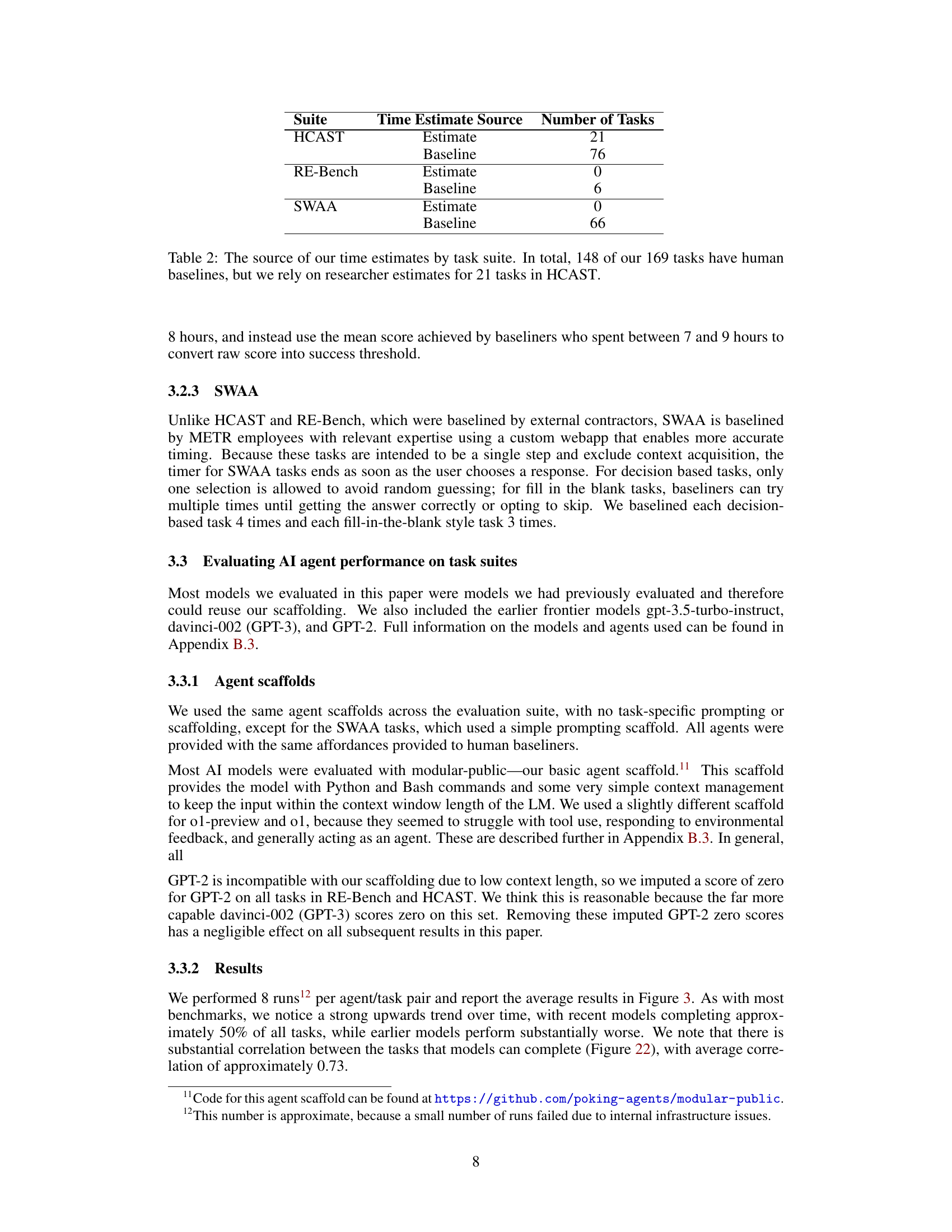
| Suite | Time Estimate Source | Number of Tasks |
|---|---|---|
| HCAST | Estimate | 21 |
| Baseline | 76 | |
| RE-Bench | Estimate | 0 |
| Baseline | 6 | |
| SWAA | Estimate | 0 |
| Baseline | 66 |
🔼 This table summarizes the source of time estimates used for the tasks in the three datasets: HCAST, RE-Bench, and SWAA. It indicates whether the time estimates were based on human performance data (baselines) or on researcher estimations. The table highlights that while the majority of tasks (148 out of 169) have human baseline timings, a smaller subset of HCAST tasks (21) relied on researcher estimates due to lack of human baseline data for those specific tasks. This distinction is crucial for understanding the reliability and potential biases in the time estimates used for analysis.
read the caption
Table 2: The source of our time estimates by task suite. In total, 148 of our 169 tasks have human baselines, but we rely on researcher estimates for 21 tasks in HCAST.
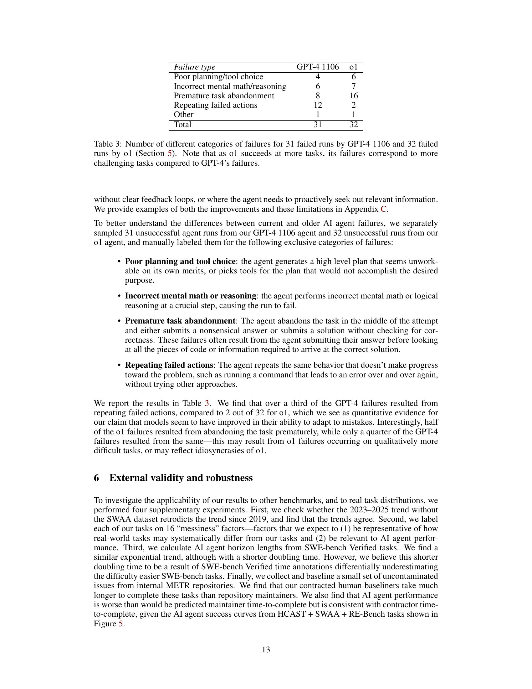
| Failure type | GPT-4 1106 | o1 |
|---|---|---|
| Poor planning/tool choice | 4 | 6 |
| Incorrect mental math/reasoning | 6 | 7 |
| Premature task abandonment | 8 | 16 |
| Repeating failed actions | 12 | 2 |
| Other | 1 | 1 |
| Total | 31 | 32 |
🔼 This table presents a breakdown of failure types for two large language models (LLMs): GPT-4 1106 and o1. It categorizes the reasons why these models failed to complete certain tasks, providing insights into the types of errors each model is prone to. The analysis reveals that the nature of the failed tasks differs between the two models; o1, being a more advanced model, tends to fail on more challenging tasks than GPT-4 1106. The failure categories include poor planning or tool selection, incorrect reasoning, premature task abandonment, and repetitive failed actions. By comparing the failure modes, researchers can gain insights into the strengths and weaknesses of each LLM and inform further model development.
read the caption
Table 3: Number of different categories of failures for 31 failed runs by GPT-4 1106 and 32 failed runs by o1 (Section 5). Note that as o1 succeeds at more tasks, its failures correspond to more challenging tasks compared to GPT-4’s failures.
| Issue | Agent | Time taken | Score |
|---|---|---|---|
| 1 | Repository Maintainer | 5 minutes | 1.0 |
| Baseliner | 81 minutes | 1.0 | |
| 8 | Repository Maintainer | 20 minutes | 1.0 |
| Baseliner | 113 minutes | 0.25 |
🔼 This table presents the results from human baseliners and repository maintainers resolving five internal pull requests (PRs). For each PR, it shows the time taken by both repository maintainers (who have more context and expertise) and baseliners (who represent a more typical external contractor) to complete the tasks, along with a manually assigned score reflecting the quality of the solution. The significant differences in time taken highlight the substantial context advantage repository maintainers possess.
read the caption
Table 4: Results of baselines on selected internal PRs
| Task ID | GPT-4o | Claude 3.5 Sonnet | o1 |
|---|---|---|---|
| Issue 1 | 0.35 (5) | 0.45 (5) | 0.875 (6) |
| Issue 8 | 0.0 (5) | 0.0 (5) | 0.0 (5) |
| Issue 9-1 | 0.0 (5) | 0.0 (5) | 0.0 (5) |
| Issue 9-2 | 0.0 (5) | 1.0 (5) | 0.85 (5) |
| Issue 10 | 0.0 (5) | 0.0 (5) | 0.0 (5) |
| Issue 11 | 0.02 (12) | 0.0 (11) | 0.0 (8) |
🔼 This table presents the average success scores achieved by three different AI models (GPT-4 0, Claude 3.5 Sonnet, and o1) on five internal pull requests (PRs). The scores represent the average performance across multiple trials for each model-task pairing. Notably, Issue 9 was divided into two separate sub-issues because its original description encompassed distinct tasks.
read the caption
Table 5: Internal PR Per-Task Average Scores (number of trials in parentheses). Note that we did minimal processing on Issue 9 to turn it into two issues, as in practice the issue description contained two entirely separate pieces of work.
| Task ID | Maintainer Time (min) | Baseliner Time (min) | Slowdown |
|---|---|---|---|
| eval-analysis-public-1 | 5 | 81 (score 1) | 16x |
| eval-analysis-public-8 | 20 | 113 (score .25) | 5.5x |
| eval-analysis-public-9-1 | 235 | - | - |
| eval-analysis-public-9-2 | 5 | 69 (score 1)* | 14x |
| eval-analysis-public-10 | 20 | - | - |
| eval-analysis-public-11 | 5 | 93 (score .75) | 18.6x |
| *Note: This was run on a slight variant | |||
🔼 This table compares the time taken by repository maintainers and external baseliners to resolve issues in an internal METR repository. It highlights the significant difference in time taken, showing that maintainers are substantially faster (5-18x) than baseliners, suggesting that baseliner performance may not be a good predictor of how well an AI system would perform the same task. The table also includes a breakdown of time taken for specific tasks and the corresponding success scores.
read the caption
Table 6: Comparison of time to fix issues by repo maintainers and baseliners
| Model | Agent |
|---|---|
| Claude 3.5 Sonnet (Old) | modular-public |
| Claude 3.5 Sonnet (New) | modular-public |
| Claude 3 Opus | modular-public |
| davinci-002 | modular-public |
| gpt-3.5-turbo-instruct | modular-public |
| GPT-4 0314 | modular-public |
| GPT-4 0125 | modular-public |
| GPT-4 1106 | modular-public |
| GPT-4 Turbo | modular-public |
| GPT-4o | modular-public |
| o1 | triframe |
| o1-preview | duet |
🔼 This table lists the different AI models used in the paper’s experiments and the specific scaffolding or framework used for each model. The scaffolding refers to the code and setup used to allow the model to interact with the task environment and execute the tasks. Different scaffolds may provide different capabilities and affordances to the models, which could influence their performance.
read the caption
Table 7: Scaffolding used for or each model in this report
| Task Time Bucket | Task Time Estimate | Average Baseline Time |
|---|---|---|
| min fix | 3.9 min | 32.9 min |
| 15 min–1 hour | 30.0 min | – |
| 1–4 hours | 120.0 min | 131.6 min |
| hours | 480.0 min | – |
🔼 Table 8 presents the conversion of time estimates from the SWE-bench Verified dataset. The dataset provides time ranges (buckets) for task completion, rather than precise times. To create a single estimate for each task, the geometric mean of the minimum and maximum times within each bucket was calculated. However, this method likely underestimates the actual time a human would take to complete these tasks, especially for tasks in the shortest time bucket (’<15 minutes’). As an example, the geometric mean across a sample of four tasks from the shortest bucket was 32.9 minutes, significantly longer than the bucket’s upper bound of 15 minutes, highlighting potential bias in the annotation method.
read the caption
Table 8: We convert the SWE-bench Verified time annotations into task estimates, by taking the geometric mean of the time annotation. We caution that this likely underestimates the time each issue takes to resolve by a human baseliner without context—notably, we observe that the geometric mean of baseliner time for four randomly sampled tasks in the “<15absent15<15< 15 minute fix” bucket is 32.9 minutes.
| Model |
|
|
| ||||||||
|---|---|---|---|---|---|---|---|---|---|---|---|
| Claude 3 Opus | 6.42 min | 0.83 min | 7.8x | ||||||||
| GPT-4 1106 | 8.56 min | 1.18 min | 7.2x | ||||||||
| GPT-4o | 9.17 min | 5.96 min | 1.5x | ||||||||
| Claude 3.5 Sonnet (Old) | 18.22 min | 5.91 min | 3.1x | ||||||||
| Claude 3.5 Sonnet (New) | 28.98 min | 16.88 min | 1.7x | ||||||||
| o1 | 39.21 min | 51.21 min | 0.8x |
🔼 This table compares the time horizons of several language models on two different benchmark suites: the authors’ task suite and SWE-bench Verified. The time horizon represents the length of tasks a model can complete with a 50% success rate. The table shows that less capable models have substantially longer time horizons on the authors’ tasks than on SWE-bench Verified, suggesting a possible difference in task difficulty or model calibration between the two benchmarks.
read the caption
Table 9: The time horizon of less capable models is substantially longer on our tasks than on SWE-bench Verified.
| Model Time |
| Horizon |
| (Our Tasks) |
🔼 This table defines eight factors used to assess the complexity and realism of tasks. These factors move beyond simple metrics like task length, evaluating characteristics such as reliance on real-world knowledge, the availability of resources, the possibility of irreversible errors, dynamic environments, and the complexity of scoring. The goal is to better understand how these characteristics might impact the performance of AI agents and influence the generalizability of benchmark results to real-world situations.
read the caption
Table 10: Messiness Factor Definitions 1-8
| Model Time |
| Horizon |
| (SWE-bench Verified) |
🔼 This table provides detailed definitions for messiness factors 9 through 16, which are used to assess the complexity and realism of tasks in the study. Each factor is defined with a clear description of what constitutes a high score for that messiness factor, along with examples to illustrate the concept. The factors help quantify aspects beyond simple task duration, considering elements like the clarity of instructions, need for real-time coordination, and the presence of implicit requirements or hidden information.
read the caption
Table 11: Messiness Factor Definitions 9-16
Full paper#