TL;DR#
Current evaluations of code-generating language models often overlook their ability to understand and produce code that satisfies specific time and space complexity constraints. This oversight leads to a gap between theoretical performance and real-world applicability, where efficiency and scalability are often critical. The ability to optimize and control computational complexity separates novice programmers from experienced ones, yet existing benchmarks do not adequately assess this higher-level reasoning skill in language models.
To address this gap, this paper introduces BIGO(BENCH), a novel coding benchmark designed to evaluate the capabilities of generative language models in understanding and generating code with specified complexities. The benchmark comprises tooling to infer algorithmic complexity, a set of 3,105 coding problems and 1,190,250 solutions annotated with time and space complexity labels. The study evaluates multiple state-of-the-art language models, revealing strengths and weaknesses in handling complexity requirements. Token-space reasoning models excel in code generation but lack complexity understanding.
Key Takeaways#
Why does it matter?#
This research introduces a novel benchmark for code LLMs to promote the development of more robust and reliable code generation models, which is important for real-world applications with complexity constraints. It opens up new research avenues to explore code LLMs in a more nuanced way.
Visual Insights#

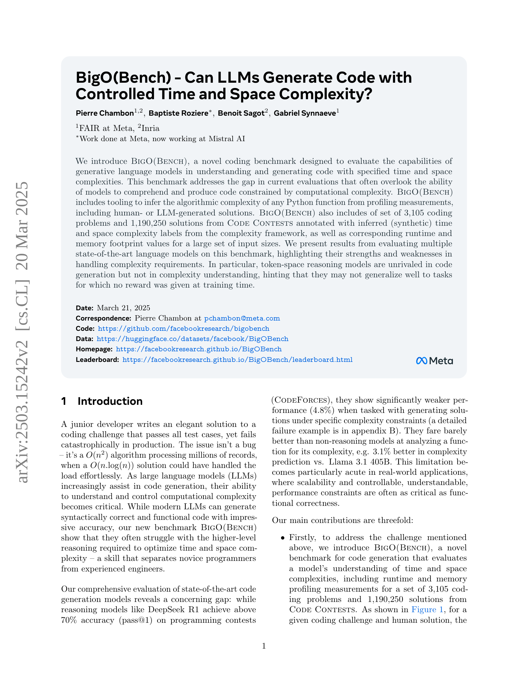
🔼 The figure illustrates the BigO(Bench) framework, which evaluates large language models (LLMs) on their ability to handle code complexity. Given a coding problem and existing human-generated solutions, BigO(Bench) assesses the LLMs’ performance in three areas: (1) predicting the time and space complexity of the solutions, (2) generating new code that satisfies specified complexity constraints, and (3) ranking solutions based on their complexity compared to human solutions. The framework uses profiling to automatically verify the LLMs’ responses by analyzing runtime distributions and curve coefficients.
read the caption
Figure 1: BigO(Bench) framework overview: Given a coding problem and human solutions, the framework evaluates language models on three key tasks: (1) predicting time-space complexities of existing solutions, (2) generating new code that meets specified complexity requirements, and (3) ranking solutions against human-written code with similar complexity profiles. The complexity framework automatically validates model outputs by computing runtime distributions and curve coefficients.
| Model | Corr | BckTr |
|---|---|---|
| Codestral 22B | 63.6 | 54.0 |
| CodeLlama 34B Instruct | 22.1 | 17.8 |
| CodeLlama 70B Instruct | 10.3 | 7.9 |
| Llama 3.1 8B Instruct | 31.9 | 21.4 |
| Llama 3.1 405B Instruct | 70.2 | 58.1 |
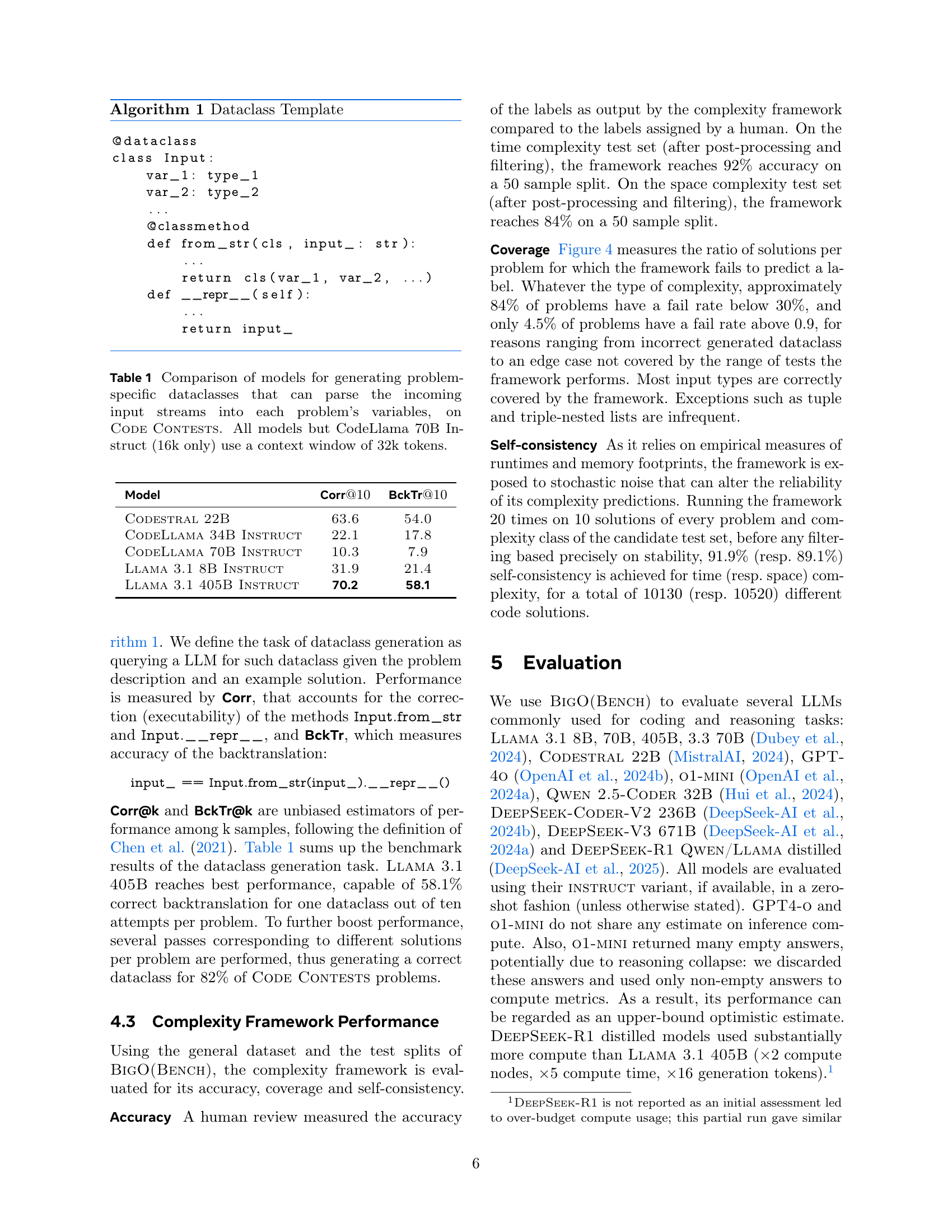
🔼 This table compares the performance of various large language models (LLMs) in generating problem-specific dataclasses for the Code Contests dataset. These dataclasses are crucial for parsing the input streams associated with each coding problem into its respective variables. The comparison focuses on the accuracy of the generated dataclasses, measuring both their correctness and the accuracy of the back-translation (whether the original input can be reconstructed from the generated dataclass). The models’ performance is evaluated using two metrics: Corr@k and BckTr@k (explained in the paper), providing a comprehensive assessment of their ability to handle this specific code generation task. Most models utilize a context window of 32k tokens; however, CodeLlama 70B Instruct is the exception, using a smaller 16k token window.
read the caption
Table 1: Comparison of models for generating problem-specific dataclasses that can parse the incoming input streams into each problem’s variables, on Code Contests. All models but CodeLlama 70B Instruct (16k only) use a context window of 32k tokens.
In-depth insights#
LLM Time Sense?#
While not explicitly stated as ‘LLM Time Sense?’, this paper indirectly explores the capacity of LLMs to reason about time, specifically computational complexity (time and space). The findings reveal that LLMs, even advanced models, exhibit limitations in understanding and generating code that adheres to specified complexity constraints. Their performance on time complexity generation tasks is significantly lower than their ability to synthesize code for general programming challenges. This suggests a deficiency in the ’time sense’ of LLMs, their ability to reason effectively about algorithmic efficiency. This deficiency hints that performance gains on benchmarks may be through memorization and not true reasoning, impacting the trustworthiness and generalization of LLMs in practical software development where scalability is crucial, and emphasizes the need for benchmarks focusing on computational complexity.
Big-O Benchmark#
The Big-O benchmark, introduced in the paper, is a novel coding challenge that assesses generative language models’ ability to understand and generate code with specified time and space complexities, addressing a critical gap in current evaluations that often overlook computational complexity. It includes a tool for inferring algorithmic complexity from profiling measurements and a dataset of coding problems with inferred complexity labels and runtime/memory footprint values, enabling a comprehensive evaluation of language models’ strengths and weaknesses in handling complexity requirements. The benchmark highlights the limitations of token-space reasoning models, which excel in code generation but not complexity understanding, suggesting potential issues in generalizing to tasks without explicit rewards during training, underscoring the importance of controlling computational complexity in code generation.
Dynamic Analysis#
Dynamic analysis, a cornerstone of code understanding, involves executing code to observe its behavior in real-time. This approach is crucial for identifying runtime complexities, performance bottlenecks, and potential inefficiencies that static analysis might miss. By profiling execution time and memory usage under various input sizes, a complexity profile can be built, effectively mapping resource consumption to input scale. The inference might be conducted by measuring runtime and memory which can be used to infer time and space complexities dynamically and identify the most effective algorithm. This technique also aids in discerning subtle optimizations and contrasting them with theoretical complexities which improves scalability and helps in optimizing the actual performance in coding challenges.
Data Generation#
While the paper doesn’t explicitly have a section titled ‘Data Generation,’ the discussion around benchmark creation and the complexity framework heavily implies a data generation strategy. The researchers generated a synthetic dataset of code solutions with associated time and space complexity labels. This was done by profiling existing code solutions from CODE CONTESTS, effectively creating a dataset where the ‘ground truth’ complexity is empirically derived rather than theoretically assigned. This approach is valuable because it reflects real-world coding practices and the performance characteristics of Python code under CPython. The framework also automatically generates variations of code solutions during its analysis phase, which is a form of data augmentation to better understand the scaling behavior of the code. This generation process also extends to creating diverse input data for functions, systematically increasing input sizes to observe the impact on runtime and memory usage. However, the lack of explicit control or targeted generation of specific complexity classes might be a limitation, potentially leading to biases in the dataset’s distribution.
Limits to Scale?#
Scalability limits in LLMs are multifaceted, encompassing computational constraints, data availability, and architectural bottlenecks. Training demands grow exponentially with model size, potentially hitting hardware limits. Data scarcity for certain domains restricts generalization. Architecturally, attention mechanisms face quadratic complexity, hindering long-context processing. Addressing these limits requires innovative approaches, such as model parallelism, efficient attention variants (e.g., sparse attention), and knowledge distillation. Furthermore, algorithmic breakthroughs and hardware advancements are crucial for pushing the boundaries of LLM scalability while maintaining performance and practicality. Balancing resource investment with expected return also plays a vital role in pushing scale further.
More visual insights#
More on figures

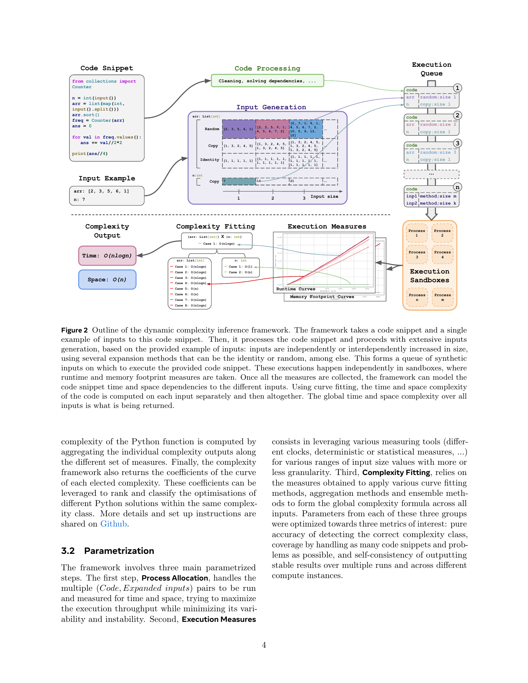
🔼 The dynamic complexity inference framework analyzes code complexity. It starts with a code snippet and sample inputs. These inputs are systematically expanded using various methods (identity, random, etc.) creating a queue of test cases. Each test case runs in isolation within a sandboxed environment, capturing runtime and memory usage. The collected data reveals the relationship between input size and resource consumption. Curve fitting techniques determine time and space complexity for each individual test and these are combined for a final, overall complexity assessment.
read the caption
Figure 2: Outline of the dynamic complexity inference framework. The framework takes a code snippet and a single example of inputs to this code snippet. Then, it processes the code snippet and proceeds with extensive inputs generation, based on the provided example of inputs: inputs are independently or interdependently increased in size, using several expansion methods that can be the identity or random, among else. This forms a queue of synthetic inputs on which to execute the provided code snippet. These executions happen independently in sandboxes, where runtime and memory footprint measures are taken. Once all the measures are collected, the framework can model the code snippet time and space dependencies to the different inputs. Using curve fitting, the time and space complexity of the code is computed on each input separately and then altogether. The global time and space complexity over all inputs is what is being returned.

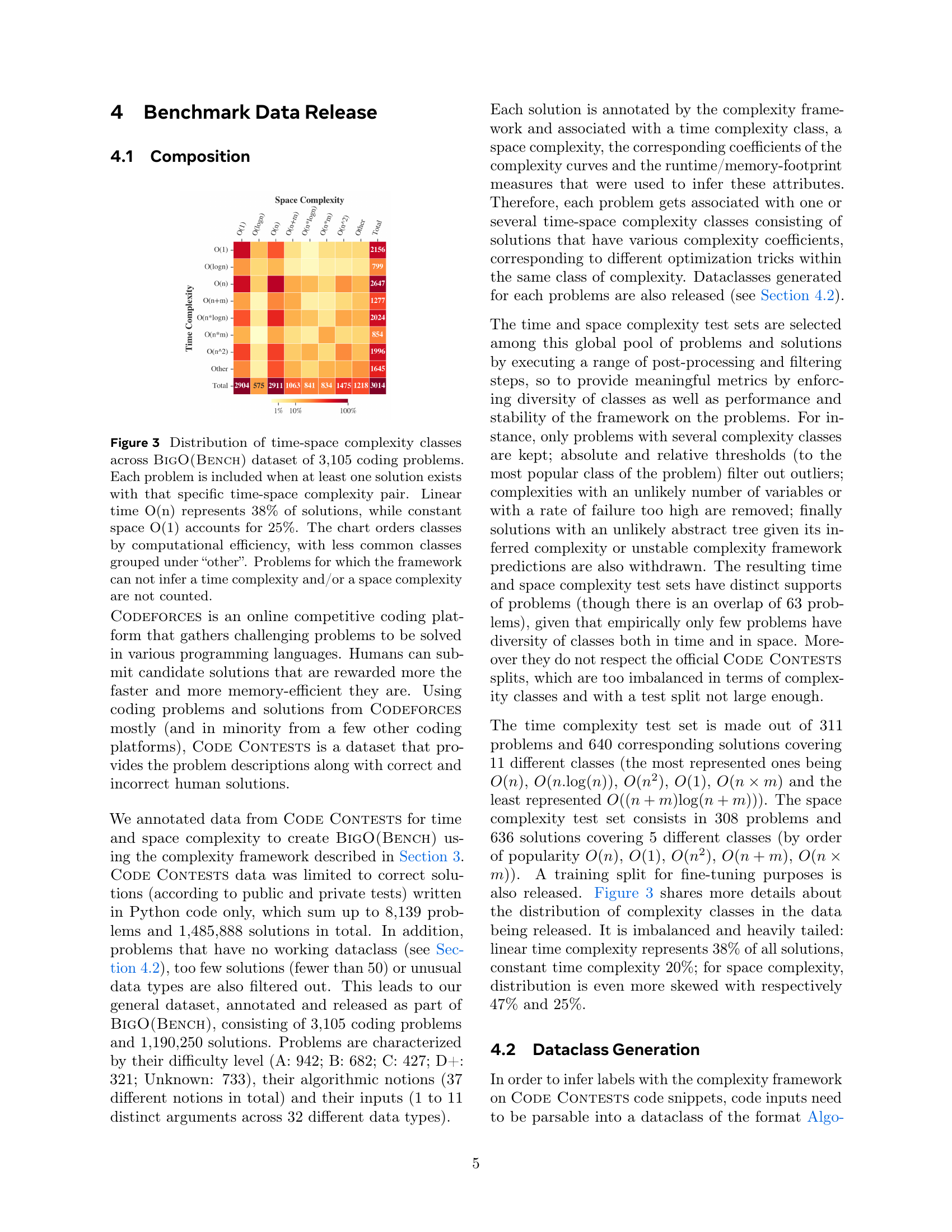
🔼 This figure visualizes the distribution of time and space complexity classes within the BigO(Bench) dataset, which comprises 3,105 coding problems. Each problem is represented if at least one solution exists matching a specific time-space complexity pair. The visualization highlights the prevalence of certain complexities: linear time complexity, O(n), accounts for 38% of the solutions, whereas constant space complexity, O(1), represents 25%. Complexities are ordered from most to least computationally efficient, with less frequent complexities grouped under the ‘other’ category. Problems where the complexity framework couldn’t determine either time or space complexity are excluded from this analysis.
read the caption
Figure 3: Distribution of time-space complexity classes across BigO(Bench) dataset of 3,105 coding problems. Each problem is included when at least one solution exists with that specific time-space complexity pair. Linear time O(n) represents 38% of solutions, while constant space O(1) accounts for 25%. The chart orders classes by computational efficiency, with less common classes grouped under “other”. Problems for which the framework can not infer a time complexity and/or a space complexity are not counted.

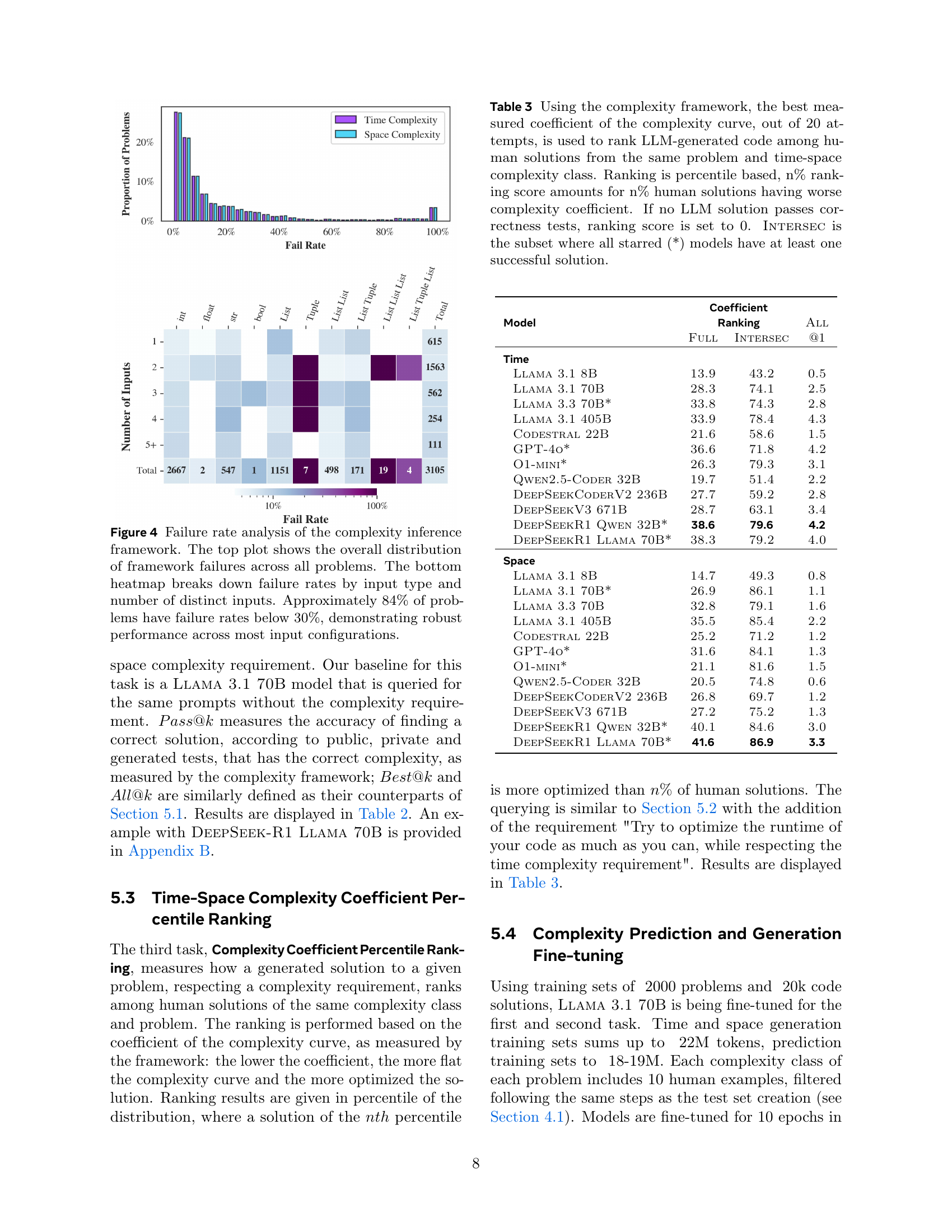
🔼 This figure analyzes the performance of the complexity inference framework. The top graph displays the distribution of problems with different failure rates, showing that 84% of problems have failure rates under 30%. The bottom heatmap provides a more detailed breakdown of failure rates based on the type and number of inputs used in each problem. This visualization highlights the framework’s robustness across various input configurations.
read the caption
Figure 4: Failure rate analysis of the complexity inference framework. The top plot shows the overall distribution of framework failures across all problems. The bottom heatmap breaks down failure rates by input type and number of distinct inputs. Approximately 84% of problems have failure rates below 30%, demonstrating robust performance across most input configurations.

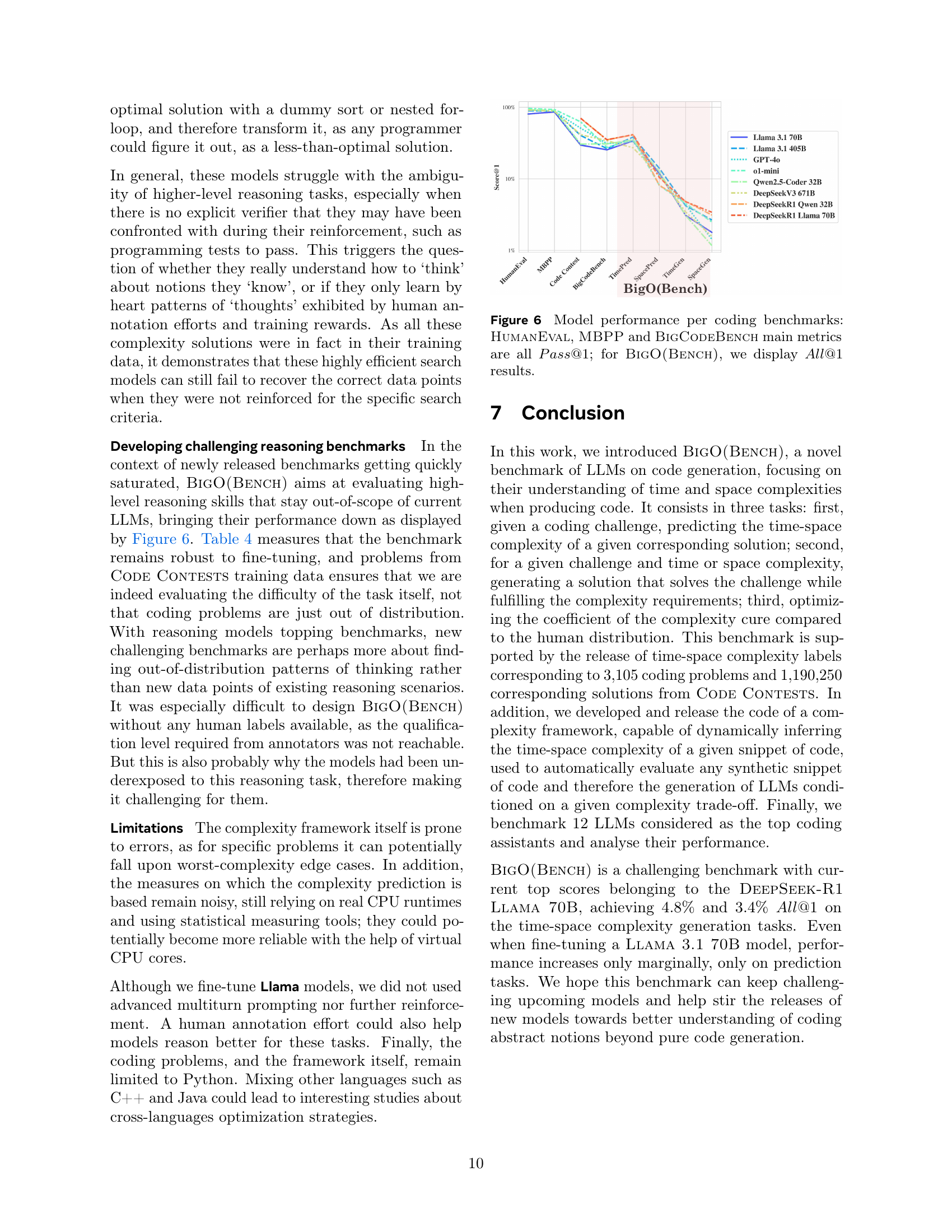
🔼 This figure visualizes the performance of various Large Language Models (LLMs) on code generation tasks categorized by time complexity and algorithmic approaches. The x-axis represents different algorithmic categories used in the problems (e.g., graph algorithms, string manipulation, etc.). The y-axis represents the accuracy or success rate of the LLMs. Different colored bars represent the various LLMs included in the benchmark. The figure allows for a comparison of LLM performance across various problem types and complexities, highlighting strengths and weaknesses of different models in handling specific algorithmic challenges.
read the caption
Figure 5: LLM results aggregated by time complexity class and by algorithmic notions for all models part of BigO(Bench).

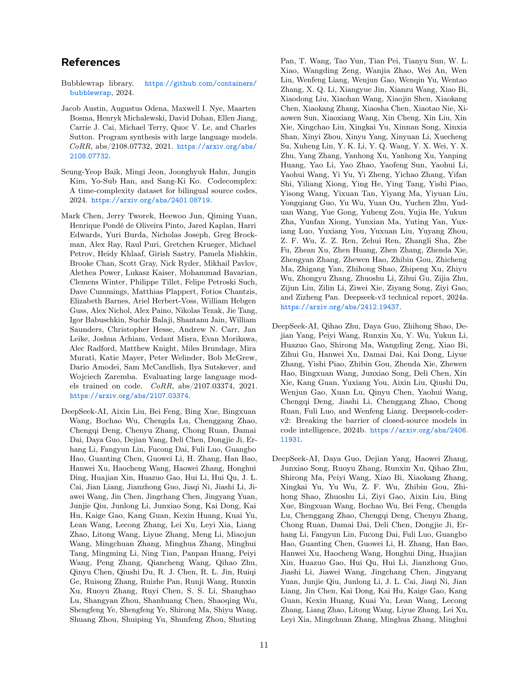
🔼 Figure 6 compares the performance of various large language models (LLMs) across four different coding benchmarks: HumanEval, MBPP, BigCodeBench, and BigO(Bench). HumanEval, MBPP, and BigCodeBench evaluate the models’ ability to generate correct code solutions to programming problems, using the Pass@1 metric which measures the percentage of problems for which the model produces the correct solution on its first try. In contrast, BigO(Bench) assesses not only the correctness but also the efficiency (time and space complexity) of the generated solutions. The BigO(Bench) results utilize the All@1 metric, indicating whether the model successfully generates correct code solutions for all problems while adhering to specific time and space constraints. The figure thus provides a comprehensive overview of LLM capabilities in terms of both code generation accuracy and algorithmic efficiency.
read the caption
Figure 6: Model performance per coding benchmarks: HumanEval, MBPP and BigCodeBench main metrics are all Pass@1𝑃𝑎𝑠𝑠@1Pass@1italic_P italic_a italic_s italic_s @ 1; for BigO(Bench), we display All@1𝐴𝑙𝑙@1All@1italic_A italic_l italic_l @ 1 results.
More on tables
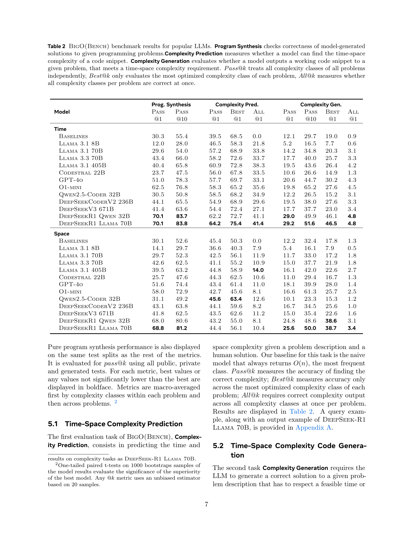
| Model | Prog. Synthesis | Complexity Pred. | Complexity Gen. | |||||||||
|---|---|---|---|---|---|---|---|---|---|---|---|---|
| Pass | Pass | Pass | Best | All | Pass | Pass | Best | All | ||||
| Time | ||||||||||||
| Baselines | 30.3 | 55.4 | 39.5 | 68.5 | 0.0 | 12.1 | 29.7 | 19.0 | 0.9 | |||
| Llama 3.1 8B | 12.0 | 28.0 | 46.5 | 58.3 | 21.8 | 5.2 | 16.5 | 7.7 | 0.6 | |||
| Llama 3.1 70B | 29.6 | 54.0 | 57.2 | 68.9 | 33.8 | 14.2 | 34.8 | 20.3 | 3.1 | |||
| Llama 3.3 70B | 43.4 | 66.0 | 58.2 | 72.6 | 33.7 | 17.7 | 40.0 | 25.7 | 3.3 | |||
| Llama 3.1 405B | 40.4 | 65.8 | 60.9 | 72.8 | 38.3 | 19.5 | 43.6 | 26.4 | 4.2 | |||
| Codestral 22B | 23.7 | 47.5 | 56.0 | 67.8 | 33.5 | 10.6 | 26.6 | 14.9 | 1.3 | |||
| GPT-4o | 51.0 | 78.3 | 57.7 | 69.7 | 33.1 | 20.6 | 44.7 | 30.2 | 4.3 | |||
| O1-mini | 62.5 | 76.8 | 58.3 | 65.2 | 35.6 | 19.8 | 65.2 | 27.6 | 4.5 | |||
| Qwen2.5-Coder 32B | 30.5 | 50.8 | 58.5 | 68.2 | 34.9 | 12.2 | 26.5 | 15.2 | 3.1 | |||
| DeepSeekCoderV2 236B | 44.1 | 65.5 | 54.9 | 68.9 | 29.6 | 19.5 | 38.0 | 27.6 | 3.3 | |||
| DeepSeekV3 671B | 41.4 | 63.6 | 54.4 | 72.4 | 27.1 | 17.7 | 37.7 | 23.0 | 3.4 | |||
| DeepSeekR1 Qwen 32B | 70.1 | 83.7 | 62.2 | 72.7 | 41.1 | 29.0 | 49.9 | 46.1 | 4.8 | |||
| DeepSeekR1 Llama 70B | 70.1 | 83.8 | 64.2 | 75.4 | 41.4 | 29.2 | 51.6 | 46.5 | 4.8 | |||
| Space | ||||||||||||
| Baselines | 30.1 | 52.6 | 45.4 | 50.3 | 0.0 | 12.2 | 32.4 | 17.8 | 1.3 | |||
| Llama 3.1 8B | 14.1 | 29.7 | 36.6 | 40.3 | 7.9 | 5.4 | 16.1 | 7.9 | 0.5 | |||
| Llama 3.1 70B | 29.7 | 52.3 | 42.5 | 56.1 | 11.9 | 11.7 | 33.0 | 17.2 | 1.8 | |||
| Llama 3.3 70B | 42.6 | 62.5 | 41.1 | 55.2 | 10.9 | 15.0 | 37.7 | 21.9 | 1.8 | |||
| Llama 3.1 405B | 39.5 | 63.2 | 44.8 | 58.9 | 14.0 | 16.1 | 42.0 | 22.6 | 2.7 | |||
| Codestral 22B | 25.7 | 47.6 | 44.3 | 62.5 | 10.6 | 11.0 | 29.4 | 16.7 | 1.3 | |||
| GPT-4o | 51.6 | 74.4 | 43.4 | 61.4 | 11.0 | 18.1 | 39.9 | 28.0 | 1.4 | |||
| O1-mini | 58.0 | 72.9 | 42.7 | 45.6 | 8.1 | 16.6 | 61.3 | 25.7 | 2.5 | |||
| Qwen2.5-Coder 32B | 31.1 | 49.2 | 45.6 | 63.4 | 12.6 | 10.1 | 23.3 | 15.3 | 1.2 | |||
| DeepSeekCoderV2 236B | 43.1 | 63.8 | 44.1 | 59.6 | 8.2 | 16.7 | 34.5 | 25.6 | 1.0 | |||
| DeepSeekV3 671B | 41.8 | 62.5 | 43.5 | 62.6 | 11.2 | 15.0 | 35.4 | 22.6 | 1.6 | |||
| DeepSeekR1 Qwen 32B | 68.0 | 80.6 | 43.2 | 55.0 | 8.1 | 24.8 | 48.6 | 38.6 | 3.1 | |||
| DeepSeekR1 Llama 70B | 68.8 | 81.2 | 44.4 | 56.1 | 10.4 | 25.6 | 50.0 | 38.7 | 3.4 | |||
🔼 Table 2 presents the performance of various Large Language Models (LLMs) on BigO(Bench), a coding benchmark focusing on time and space complexity. The benchmark assesses LLMs across three key tasks: Program Synthesis (generating correct code), Complexity Prediction (identifying the time-space complexity of existing code), and Complexity Generation (creating code meeting specific time-space complexity constraints). The table shows the models’ accuracy (Pass@k, Best@k, All@k) for each task. Pass@k indicates the overall accuracy, considering each problem’s complexity class independently. Best@k focuses on accuracy only for a problem’s most efficient complexity class, while All@k measures whether all complexity classes within a problem are correctly identified.
read the caption
Table 2: BigO(Bench) benchmark results for popular LLMs. Program Synthesis checks correctness of model-generated solutions to given programming problems.Complexity Prediction measures whether a model can find the time-space complexity of a code snippet. Complexity Generation evaluates whether a model outputs a working code snippet to a given problem, that meets a time-space complexity requirement. Pass@k𝑃𝑎𝑠𝑠@𝑘Pass@kitalic_P italic_a italic_s italic_s @ italic_k treats all complexity classes of all problems independently, Best@k𝐵𝑒𝑠𝑡@𝑘Best@kitalic_B italic_e italic_s italic_t @ italic_k only evaluates the most optimized complexity class of each problem, All@k𝐴𝑙𝑙@𝑘All@kitalic_A italic_l italic_l @ italic_k measures whether all complexity classes per problem are correct at once.
| Model | Coefficient | ||
|---|---|---|---|
| Ranking | All | ||
| Full | Intersec | ||
| Time | |||
| Llama 3.1 8B | 13.9 | 43.2 | 0.5 |
| Llama 3.1 70B | 28.3 | 74.1 | 2.5 |
| Llama 3.3 70B* | 33.8 | 74.3 | 2.8 |
| Llama 3.1 405B | 33.9 | 78.4 | 4.3 |
| Codestral 22B | 21.6 | 58.6 | 1.5 |
| GPT-4o* | 36.6 | 71.8 | 4.2 |
| O1-mini* | 26.3 | 79.3 | 3.1 |
| Qwen2.5-Coder 32B | 19.7 | 51.4 | 2.2 |
| DeepSeekCoderV2 236B | 27.7 | 59.2 | 2.8 |
| DeepSeekV3 671B | 28.7 | 63.1 | 3.4 |
| DeepSeekR1 Qwen 32B* | 38.6 | 79.6 | 4.2 |
| DeepSeekR1 Llama 70B* | 38.3 | 79.2 | 4.0 |
| Space | |||
| Llama 3.1 8B | 14.7 | 49.3 | 0.8 |
| Llama 3.1 70B* | 26.9 | 86.1 | 1.1 |
| Llama 3.3 70B | 32.8 | 79.1 | 1.6 |
| Llama 3.1 405B | 35.5 | 85.4 | 2.2 |
| Codestral 22B | 25.2 | 71.2 | 1.2 |
| GPT-4o* | 31.6 | 84.1 | 1.3 |
| O1-mini* | 21.1 | 81.6 | 1.5 |
| Qwen2.5-Coder 32B | 20.5 | 74.8 | 0.6 |
| DeepSeekCoderV2 236B | 26.8 | 69.7 | 1.2 |
| DeepSeekV3 671B | 27.2 | 75.2 | 1.3 |
| DeepSeekR1 Qwen 32B* | 40.1 | 84.6 | 3.0 |
| DeepSeekR1 Llama 70B* | 41.6 | 86.9 | 3.3 |
🔼 This table presents the results of ranking LLMs’ code generation performance against human-written code for the same problem, while considering time and space complexity requirements. The ranking uses the complexity framework described in the paper. The framework evaluates 20 attempts to measure complexity for each model, choosing the best coefficient to assess performance. This assessment considers both time and space complexity. A percentile-based ranking system is employed; for instance, a ranking score of ’n%’ signifies that ’n%’ of human-generated solutions performed worse regarding the complexity coefficient. If a model failed to produce a correct solution, its ranking is zero. The ‘Intersec’ subset highlights the models (marked with *) with at least one successful solution.
read the caption
Table 3: Using the complexity framework, the best measured coefficient of the complexity curve, out of 20 attempts, is used to rank LLM-generated code among human solutions from the same problem and time-space complexity class. Ranking is percentile based, n% ranking score amounts for n% human solutions having worse complexity coefficient. If no LLM solution passes correctness tests, ranking score is set to 0. Intersec is the subset where all starred (*) models have at least one successful solution.
| Method | Prog. | Prediction | Generation | ||
|---|---|---|---|---|---|
| Synth. | Time | Space | Time | Space | |
| Pass | All | All | All | All | |
| Zero-shot | 29.6 | 33.8 | 11.9 | 3.1 | 1.8 |
| Few-shot | 28.9 | 33.6 | 12.1 | 2.4 | 1.4 |
| Prediction Fine-tuning | |||||
| Time | 27.4 | 36.5 | 6.6 | 2.9 | 1.3 |
| Space | 26.6 | 9.0 | 14.0 | 2.4 | 1.4 |
| Generation Fine-tuning | |||||
| Time | 23.2 | 34.7 | 12.7 | 1.2 | 1.3 |
| Space | 23.4 | 34.6 | 13.0 | 1.5 | 1.4 |
🔼 This table presents the results of fine-tuning the Llama 3.1 70B language model on the BigO(Bench) benchmark for time and space complexity prediction and generation tasks. It shows the model’s performance across several metrics (Pass@1, Pass@10, Best@1, Best@10, All@1, All@10) before and after fine-tuning. These metrics evaluate the accuracy of the model in correctly predicting and generating code that meets specified time and space complexity requirements. The table also compares the performance of the fine-tuned model to its zero-shot and few-shot counterparts.
read the caption
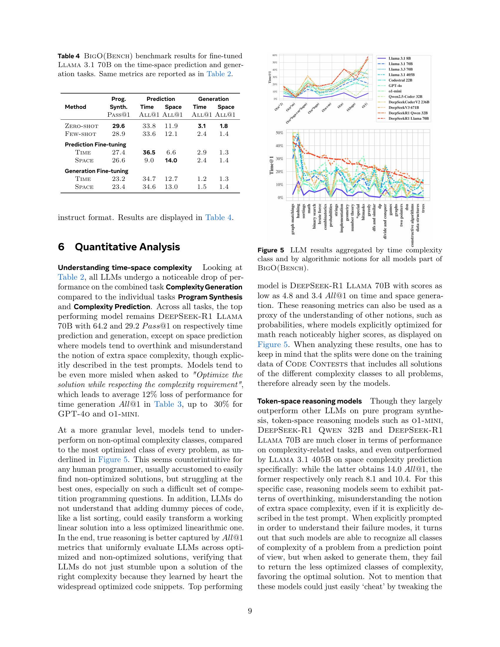
Table 4: BigO(Bench) benchmark results for fine-tuned Llama 3.1 70B on the time-space prediction and generation tasks. Same metrics are reported as in Table 2.
Full paper#