TL;DR#
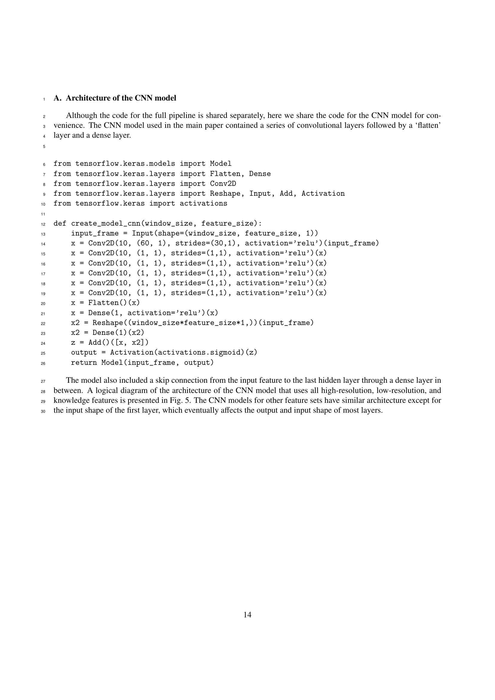
Key Takeaways#
Why does it matter?#
This research is important because it addresses a critical need for personalized adherence forecasting in healthcare. By leveraging wearable sensor data and future knowledge, it opens new avenues for developing effective intervention tools and improving patient outcomes, contributing to the growing field of mobile health and personalized medicine.
Visual Insights#

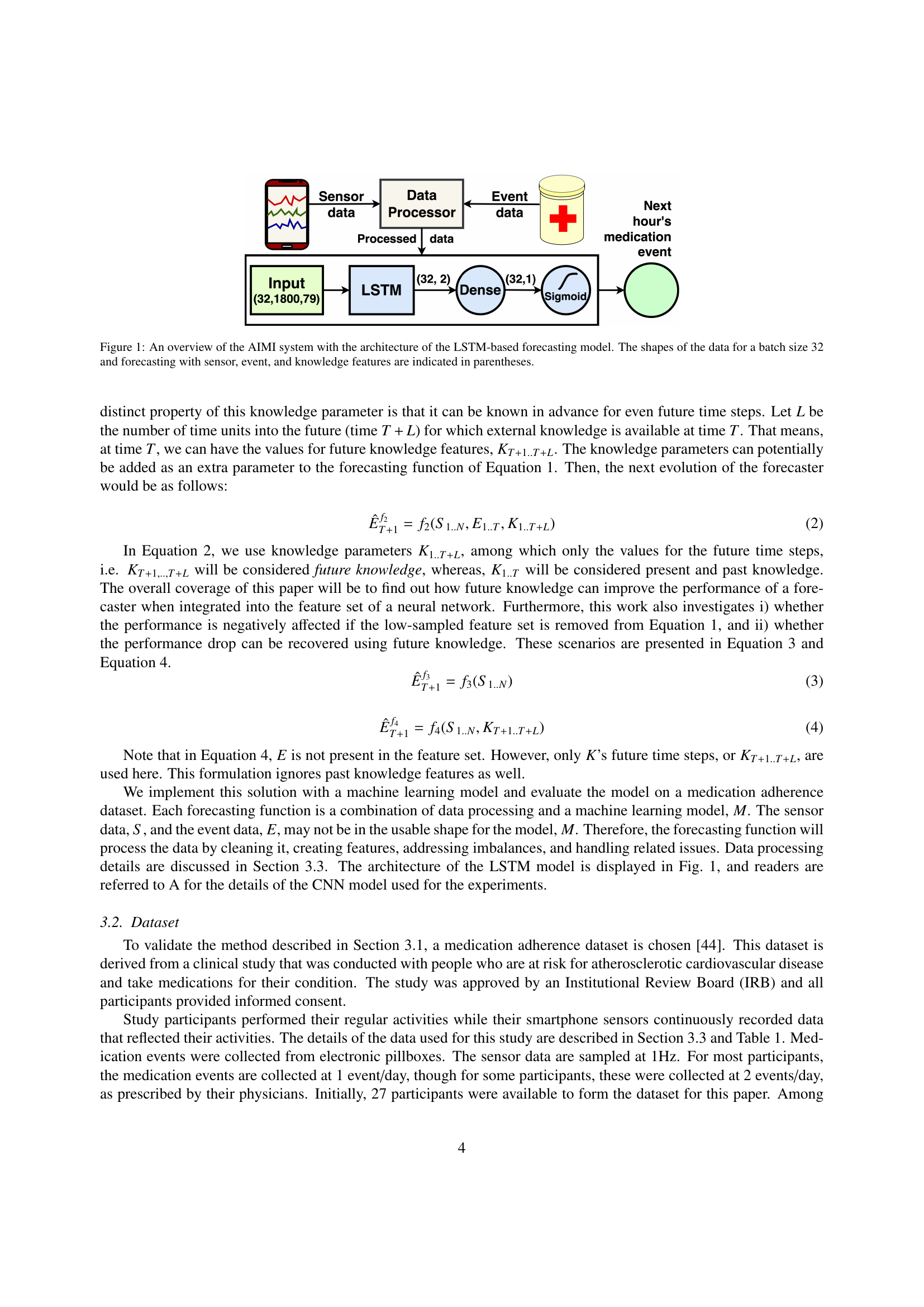
🔼 This figure illustrates the Adherence Forecasting and Intervention with Machine Intelligence (AIMI) system’s architecture, focusing on the LSTM-based forecasting model. The data flow begins with sensor data and event data being processed. The processed data, along with knowledge features, is fed into the LSTM model which then outputs a prediction for the next hour’s medication event. The parentheses display the dimensions of the input data for a batch size of 32, showing the shape of the sensor data, event data, and knowledge features.
read the caption
Figure 1: An overview of the AIMI system with the architecture of the LSTM-based forecasting model. The shapes of the data for a batch size 32 and forecasting with sensor, event, and knowledge features are indicated in parentheses.
| Feature | Type | Dimension |
|---|---|---|
| High-resolution features (H) | 14 | |
| Yaw, Pitch, Roll | N | 3 |
| Rotation rate (x,y,z) | N | 3 |
| Acceleration (x,y,z) | N | 3 |
| Latitude, longitude | N | 2 |
| Altitude, horizontal accuracy, speed | N | 3 |
| Low-resolution features (L) | 39 | |
| Last medication event | B | 1 |
| Last prescribed time | N | 1 |
| Last event hour | N | 1 |
| Day of the week | B | 7 |
| Hour of the day | B | 24 |
| Medication events of | ||
| last 2, 3, 6, 12, and 24 hours | B | 5 |
| Future knowledge features (K) | 26 | |
| Relative timestamp | N | 2 |
| Next prescribed hour | B | 24 |
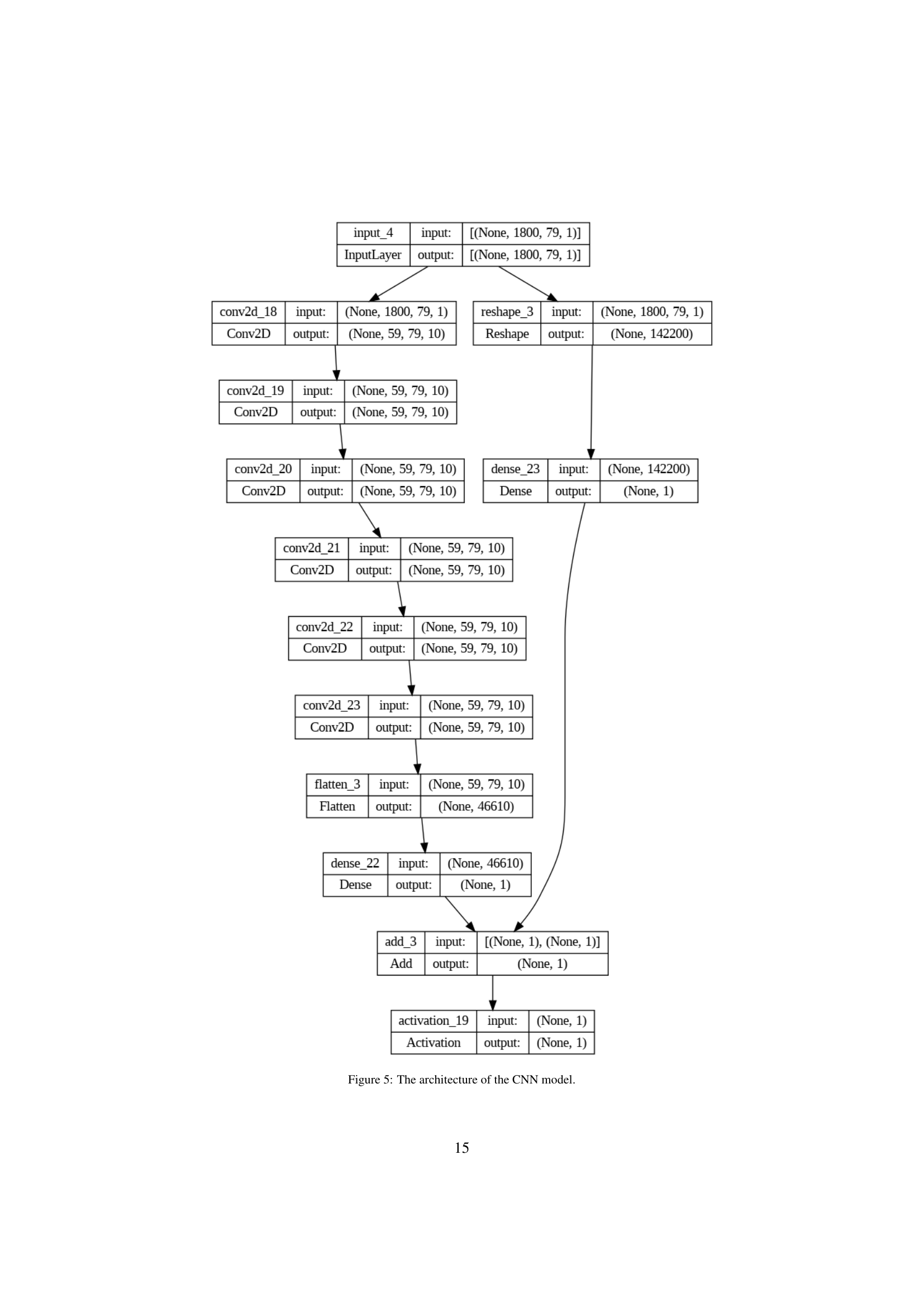
| Medication next hour (target) | B | 1 |
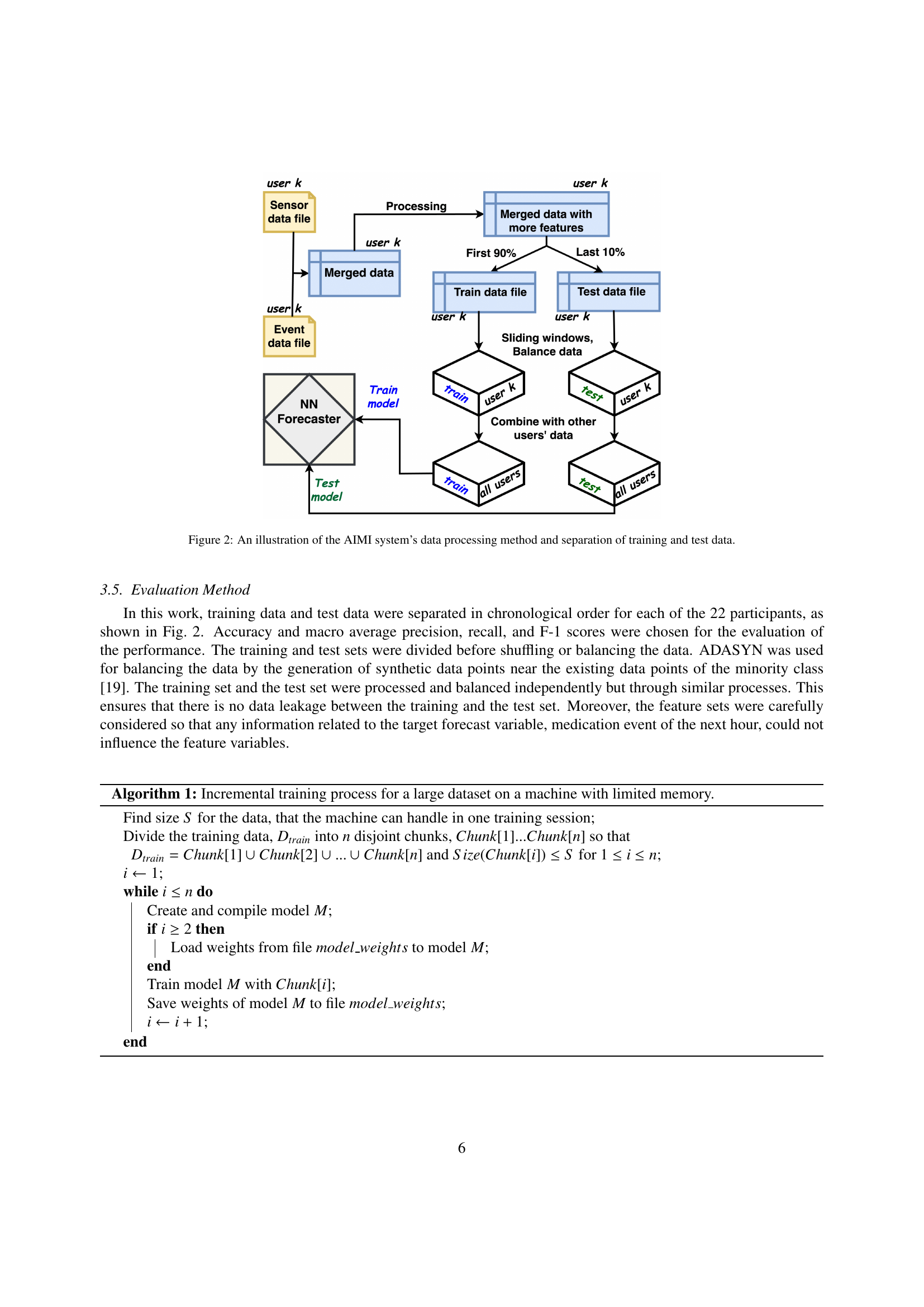
🔼 Table 1 presents the features used in the AIMI model for forecasting medication adherence. It details the type and dimensionality of each feature, categorized into high-resolution sensor data, low-resolution sensor data, and future knowledge features. The ‘Relative Timestamp’ and ‘Next Prescribed Hour’ features are particularly important because they incorporate knowledge of future events. The target variable to be predicted is ‘Medication Next Hour’, indicating whether the medication was taken in the next hour.
read the caption
Table 1: Dataset features. Here, the Relative timestamp and Next prescribed hour features embed knowledge of the future. Medication next hour is the forecast variable. Type N=numeric, B=boolean.
In-depth insights#
AIMI: Adherence#
AIMI (Adherence Forecasting and Intervention with Machine Intelligence) is an approach to improve medication adherence using technology. It leverages data from smartphone sensors and medication history to predict if someone will miss taking their medication. The core idea is to provide timely, personalized support to individuals who are at risk of non-adherence. AIMI utilizes machine learning models to analyze sensor data (activity, location) and combine it with information about prescribed medications, like dosage, frequency. The aim is to create a system that can accurately forecast treatment adherence and enable interventions, such as reminders or personalized support, to help patients stay on track. The ‘intelligence’ aspect refers to machine learning algorithms. It’s important to note that the system accounts for both current activity, past adherence, time context, and future prescription information.
Sparse Event DL#
Sparse Event Deep Learning (DL) presents unique challenges and opportunities. The “sparse” nature implies data scarcity, where events of interest are infrequent compared to background noise or irrelevant data. This necessitates specialized DL architectures and training methodologies. Data augmentation techniques become crucial to artificially inflate the event dataset, and transfer learning from related, denser datasets can bootstrap model performance. Anomaly detection approaches can be adapted, framing rare events as deviations from the norm. Careful consideration of loss functions is essential; weighted losses or focal loss can prioritize accurate classification of the sparse event class. Furthermore, DL models must be robust to the imbalanced nature of sparse event data. Specialized architectures like autoencoders or generative adversarial networks (GANs) can learn the underlying data distribution and generate synthetic events for augmentation. The goal is to extract meaningful insights from limited data, requiring careful feature engineering and algorithm selection.
Time-Series Future#
The idea of “Time-Series Future” in research is intriguing, particularly when considering predictive modeling. It suggests leveraging not only historical data but also anticipated future events to improve forecast accuracy. Incorporating future knowledge could significantly enhance the precision of models, especially in domains with scheduled events or known interventions. For example, in healthcare, knowing future medication schedules or appointments could refine adherence predictions. The challenge lies in effectively integrating this future information without introducing bias or overfitting to known events. Careful feature engineering is needed to ensure the model learns generalizable patterns rather than simply memorizing specific future occurrences. Additionally, handling uncertainty associated with future events is crucial, as predictions about the future are inherently probabilistic. The potential benefits of incorporating future knowledge into time-series models warrant further investigation, as it could lead to more robust and reliable forecasting in various fields.
CNN vs. LSTM#
When comparing CNNs and LSTMs, several factors must be considered. CNNs excel at extracting spatial features, making them suitable for tasks where local patterns are important. Their computational efficiency often allows for faster training, especially with large datasets. However, CNNs might struggle with long-range dependencies in sequential data. Conversely, LSTMs are designed to capture temporal dependencies, processing sequences step-by-step and maintaining a memory of past inputs. This makes them ideal for time-series analysis and natural language processing, but they can be computationally intensive and may require more training data. The choice between CNNs and LSTMs depends on the specific task and data characteristics. Hybrid approaches combining the strengths of both architectures are also common, leveraging CNNs for feature extraction and LSTMs for sequence modeling. Additionally, it is very important to choose the appropriate hyperparameters of each model to get the best results.
Personalization#
The section on personalization highlights the importance of tailoring treatment adherence strategies to individual needs and behaviors. Generic interventions often fall short due to the diverse factors influencing adherence, such as personal beliefs, lifestyle, and social support. Personalization involves leveraging individual data, including sensor data, adherence history, and contextual information, to create targeted interventions. This approach acknowledges that individuals respond differently to reminders, feedback, and support mechanisms. Adaptive interventions, which adjust in real-time based on individual responses, hold significant promise. Personalization further improves by addressing the parameter challanges during model training for a specific set of users. Personalized models can thus forcast better than generic, and more robust models.
More visual insights#
More on figures

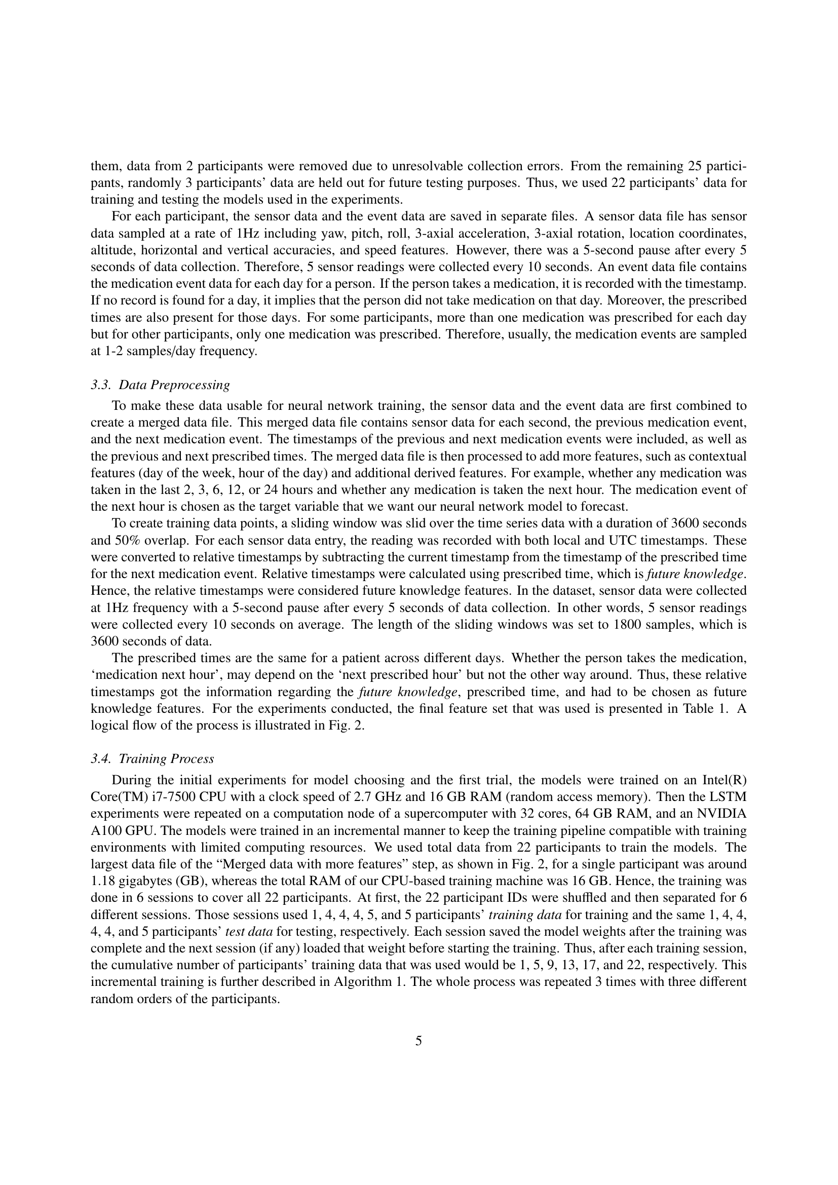
🔼 This figure illustrates the data processing pipeline used in the AIMI system. It starts with raw sensor data and event data (medication taken or missed) collected from individual users. The data is then processed to add more features like contextual information (day of week, time of day), and derived features. This enriched dataset is then split into training and testing datasets, with 90% of the data used for training and the remaining 10% for testing the prediction model. The training data is further processed using a sliding window technique to create multiple instances for model training.
read the caption
Figure 2: An illustration of the AIMI system’s data processing method and separation of training and test data.

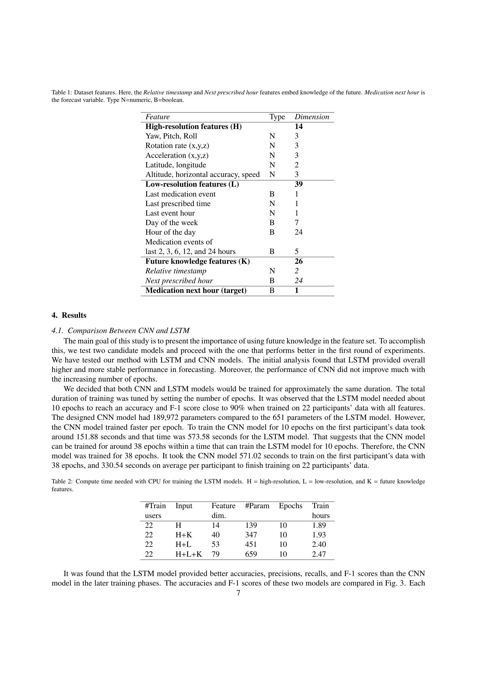
🔼 The figure shows a comparison of the CNN and LSTM models’ accuracies and F1-scores across different training phases. The x-axis represents different training phases, each labeled with the number of training and test participants involved (e.g., 1-1 indicates one training and one testing participant, while 22-5 represents 22 training and 5 testing participants). The y-axis represents the model’s performance, measured in terms of accuracy (sub-figure a) and F1-score (sub-figure b). The lines represent the performance of each model (CNN and LSTM) across various training phases. This visual helps demonstrate how the models perform with increasing amounts of training data and the relative strengths of each model in terms of accuracy and F1-score.
read the caption
(a) Accuracies

🔼 This figure shows the macro-averaged F-1 scores of the CNN and LSTM models across different training phases. The x-axis represents the training phase, indicating the number of participants used for training and testing in each phase (e.g., 1-1 means 1 participant for training and 1 for testing, while 22-5 represents 22 participants for training and 5 for testing). The y-axis represents the F-1 score, a metric that combines precision and recall, measuring the overall accuracy of the model’s predictions. The plot shows how the F-1 score changes for both CNN and LSTM models as the amount of training data increases. This illustrates the models’ performance improvement with more training data and allows for a comparison between the two model architectures.
read the caption
(b) F-1 scores

🔼 This figure compares the performance of Convolutional Neural Network (CNN) and Long Short-Term Memory (LSTM) models for forecasting medication adherence. The models were trained incrementally, adding more participants’ data in each phase. The x-axis shows the training phases, identified by the number of training and testing participants (e.g., 1-1 means 1 participant for training and 1 for testing, 5-4 means 5 for training and 4 for testing, and so on). The y-axis represents the model’s accuracy and F1-score, key metrics evaluating model performance. The figure helps to visualize how the models’ accuracy and F1-score change as more data is included in the training process. This provides insight into the effectiveness of each model and the impact of data size on prediction accuracy.
read the caption
Figure 3: Comparison of the CNN and LSTM models’ accuracies and macro average F-1 scores in different training phases. The training phase labels, 1-1, 5-4, 9-4, 13-4, 17-4, and 22-5, indicate the numbers of training and test participants for those phases.
More on tables
| #Train | Input | Feature | #Param | Epochs | Train |
|---|---|---|---|---|---|
| users | dim. | hours | |||
| 22 | H | 14 | 139 | 10 | 1.89 |
| 22 | H+K | 40 | 347 | 10 | 1.93 |
| 22 | H+L | 53 | 451 | 10 | 2.40 |
| 22 | H+L+K | 79 | 659 | 10 | 2.47 |
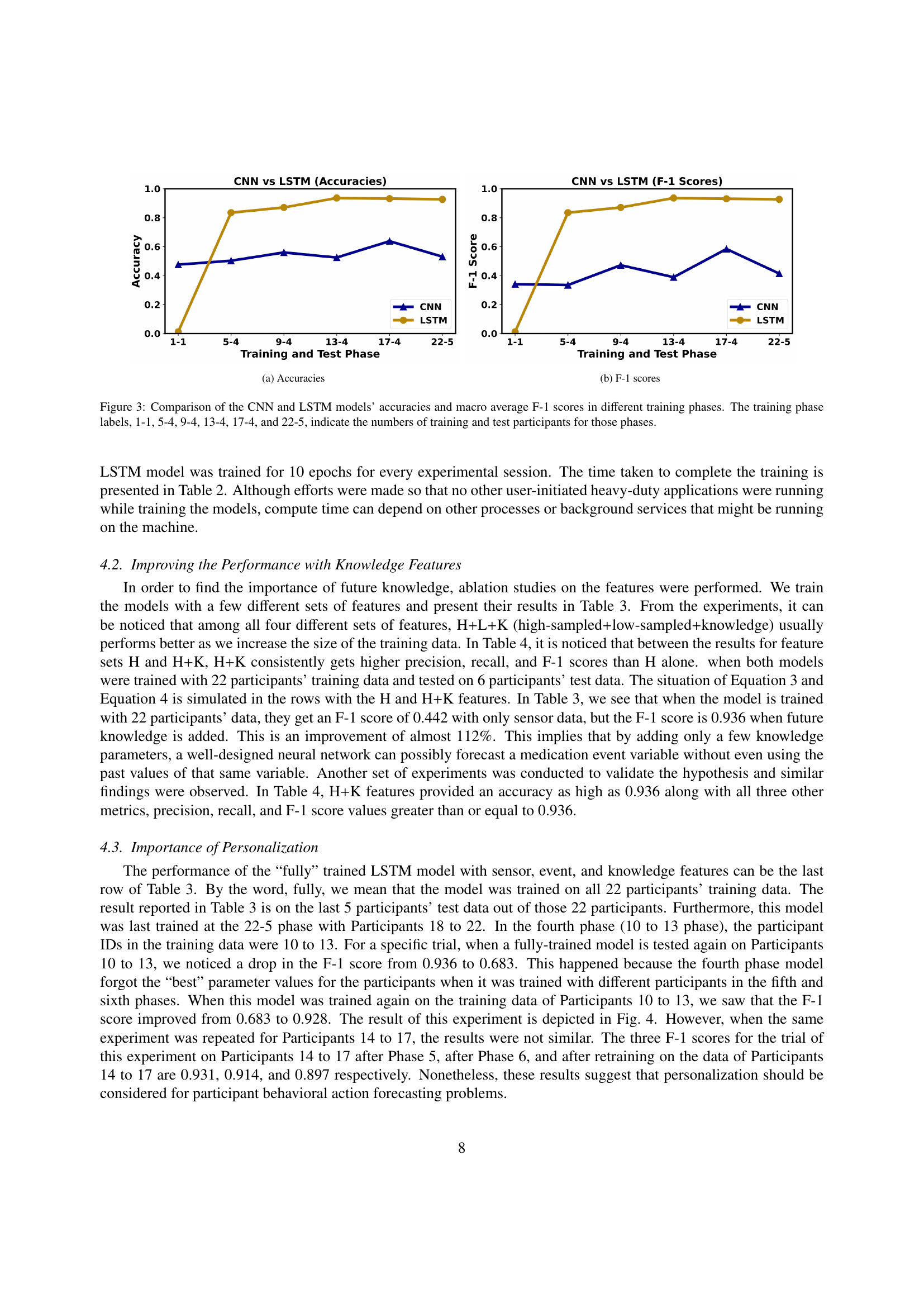
🔼 This table presents the computational time required for training LSTM models using different sets of features. The models were trained on a CPU. The table shows the number of training users, input dimensions, the features used (High-resolution (H), Low-resolution (L), and Future knowledge (K) features), the number of model parameters, the number of training epochs, and the total training time in hours. This allows for a comparison of training time across different feature combinations and model complexities.
read the caption
Table 2: Compute time needed with CPU for training the LSTM models. H = high-resolution, L = low-resolution, and K = future knowledge features.
| #Train | #Test | Features | Accuracy | Precision | Recall | F-1 |
|---|---|---|---|---|---|---|
| users | users | |||||
| 1 | 1 | H | 0.617 | 0.189 | 0.521 | 0.237 |
| 1 | 1 | H+K | 0.869 | 0.385 | 0.562 | 0.449 |
| 1 | 1 | H+L | 0.510 | 0.015 | 0.333 | 0.028 |
| 1 | 1 | H+L+K | 0.937 | 0.405 | 0.600 | 0.469 |
| 5 | 4 | H | 0.549 | 0.447 | 0.328 | 0.375 |
| 5 | 4 | H+K | 0.805 | 0.847 | 0.719 | 0.733 |
| 5 | 4 | H+L | 0.659 | 0.652 | 0.820 | 0.705 |
| 5 | 4 | H+L+K | 0.912 | 0.895 | 0.936 | 0.913 |
| 9 | 4 | H | 0.475 | 0.321 | 0.441 | 0.361 |
| 9 | 4 | H+K | 0.909 | 0.871 | 0.961 | 0.914 |
| 9 | 4 | H+L | 0.782 | 0.824 | 0.715 | 0.765 |
| 9 | 4 | H+L+K | 0.896 | 0.848 | 0.970 | 0.904 |
| 13 | 4 | H | 0.494 | 0.166 | 0.333 | 0.222 |
| 13 | 4 | H+K | 0.845 | 0.878 | 0.801 | 0.838 |
| 13 | 4 | H+L | 0.833 | 0.787 | 0.921 | 0.847 |
| 13 | 4 | H+L+K | 0.919 | 0.888 | 0.958 | 0.922 |
| 17 | 4 | H | 0.605 | 0.665 | 0.659 | 0.616 |
| 17 | 4 | H+K | 0.906 | 0.855 | 0.977 | 0.912 |
| 17 | 4 | H+L | 0.834 | 0.794 | 0.899 | 0.842 |
| 17 | 4 | H+L+K | 0.894 | 0.849 | 0.959 | 0.901 |
| 22 | 5 | H | 0.516 | 0.455 | 0.526 | 0.442 |
| 22 | 5 | H+K | 0.932 | 0.888 | 0.989 | 0.936 |
| 22 | 5 | H+L | 0.829 | 0.798 | 0.903 | 0.837 |
| 22 | 5 | H+L+K | 0.898 | 0.867 | 0.946 | 0.903 |
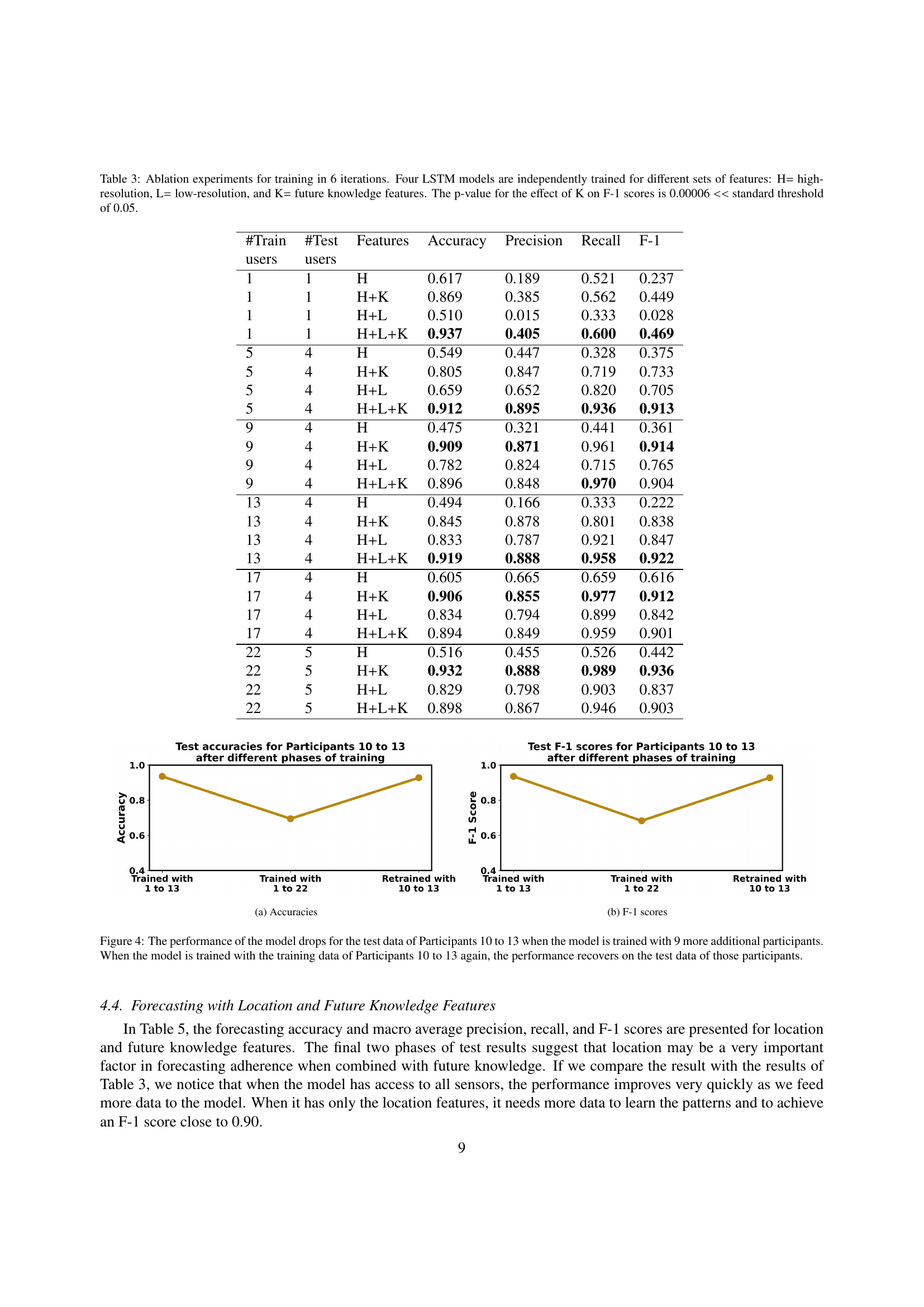
🔼 This table presents ablation study results comparing four LSTM models trained with different feature sets across six iterations. The models used high-resolution (H), low-resolution (L), and future knowledge (K) features in various combinations. The results demonstrate the impact of each feature set on model performance, measured by accuracy, precision, recall, and F1-score. A statistically significant improvement (p<0.00006) in the F1-score was observed when future knowledge features (K) were included, highlighting their importance in improving prediction accuracy.
read the caption
Table 3: Ablation experiments for training in 6 iterations. Four LSTM models are independently trained for different sets of features: H= high-resolution, L= low-resolution, and K= future knowledge features. The p-value for the effect of K on F-1 scores is 0.00006 <
| #Train | #Test | Features | Accuracy | Precision | Recall | F-1 |
|---|---|---|---|---|---|---|
| users | users | |||||
| 1 | 1 | H | 0.905 | 0.575 | 0.574 | 0.575 |
| 1 | 1 | H+K | 0.952 | 0.577 | 0.599 | 0.588 |
| 8 | 7 | H | 0.403 | 0.241 | 0.406 | 0.292 |
| 8 | 7 | H+K | 0.879 | 0.879 | 0.879 | 0.879 |
| 12 | 4 | H | 0.525 | 0.526 | 0.524 | 0.518 |
| 12 | 4 | H+K | 0.880 | 0.880 | 0.880 | 0.880 |
| 16 | 4 | H | 0.490 | 0.489 | 0.490 | 0.485 |
| 16 | 4 | H+K | 0.936 | 0.943 | 0.937 | 0.936 |
| 22 | 6 | H | 0.516 | 0.549 | 0.518 | 0.428 |
| 22 | 6 | H+K | 0.922 | 0.932 | 0.922 | 0.921 |
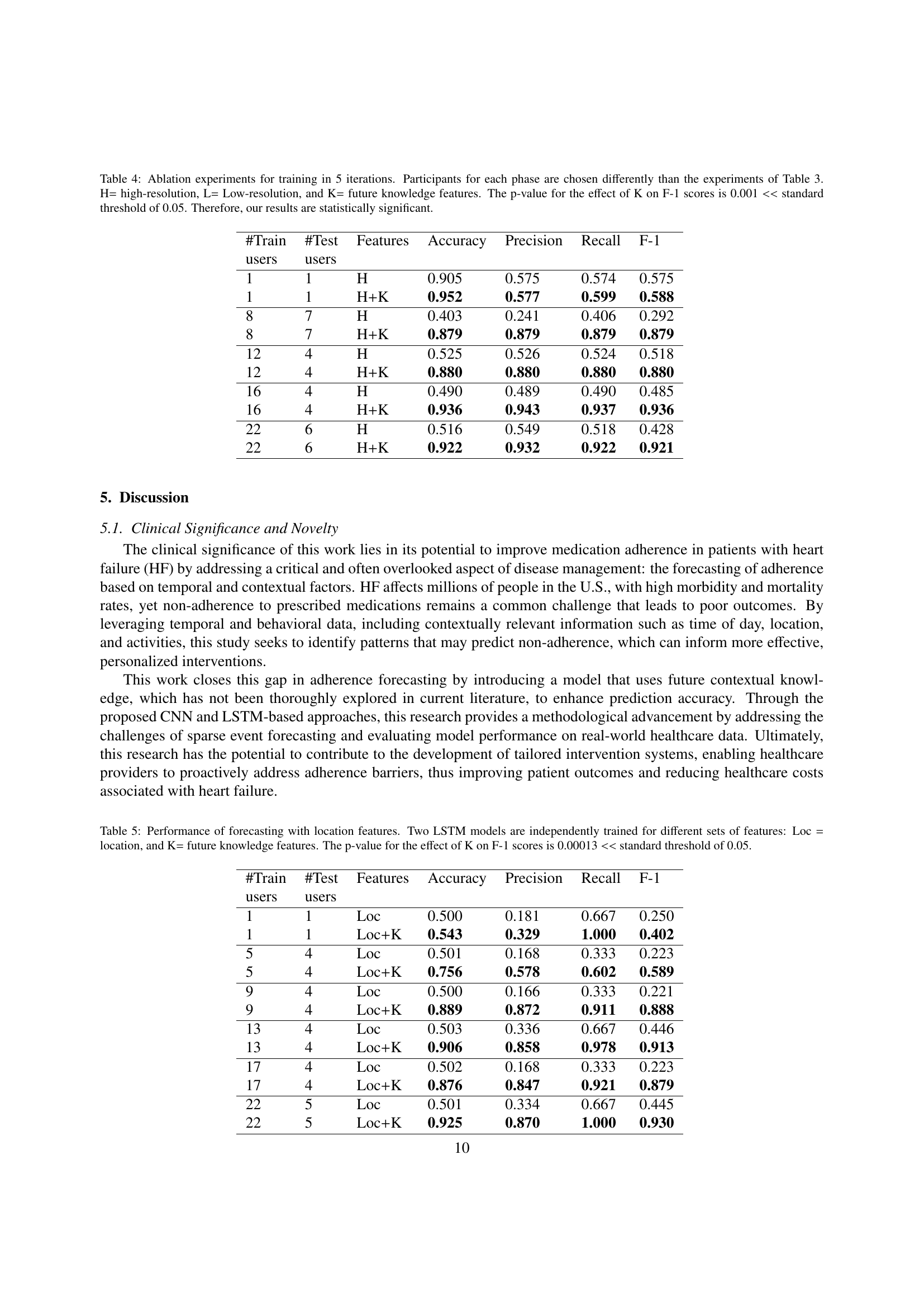
🔼 This table presents ablation study results comparing the performance of an LSTM model trained with different combinations of features (high-resolution, low-resolution, and future knowledge). The model was trained across 5 iterations, with participant data selected differently than in Table 3. The results show the impact of including future knowledge (K) features on model accuracy, precision, recall, and F1-score. Statistical significance of the impact of K on the F1-score is demonstrated using a p-value significantly below the standard threshold of 0.05.
read the caption
Table 4: Ablation experiments for training in 5 iterations. Participants for each phase are chosen differently than the experiments of Table 3. H= high-resolution, L= Low-resolution, and K= future knowledge features. The p-value for the effect of K on F-1 scores is 0.001 <
| #Train | #Test | Features | Accuracy | Precision | Recall | F-1 |
|---|---|---|---|---|---|---|
| users | users | |||||
| 1 | 1 | Loc | 0.500 | 0.181 | 0.667 | 0.250 |
| 1 | 1 | Loc+K | 0.543 | 0.329 | 1.000 | 0.402 |
| 5 | 4 | Loc | 0.501 | 0.168 | 0.333 | 0.223 |
| 5 | 4 | Loc+K | 0.756 | 0.578 | 0.602 | 0.589 |
| 9 | 4 | Loc | 0.500 | 0.166 | 0.333 | 0.221 |
| 9 | 4 | Loc+K | 0.889 | 0.872 | 0.911 | 0.888 |
| 13 | 4 | Loc | 0.503 | 0.336 | 0.667 | 0.446 |
| 13 | 4 | Loc+K | 0.906 | 0.858 | 0.978 | 0.913 |
| 17 | 4 | Loc | 0.502 | 0.168 | 0.333 | 0.223 |
| 17 | 4 | Loc+K | 0.876 | 0.847 | 0.921 | 0.879 |
| 22 | 5 | Loc | 0.501 | 0.334 | 0.667 | 0.445 |
| 22 | 5 | Loc+K | 0.925 | 0.870 | 1.000 | 0.930 |
🔼 This table presents the results of experiments evaluating the impact of location data and future knowledge features on the accuracy of medication adherence forecasting using LSTM models. Two sets of experiments are shown. One uses only location data (‘Loc’), and the other combines location data with future knowledge features (‘Loc+K’). The results (accuracy, precision, recall, and F1-score) are presented for each model across different training set sizes, ranging from 1 to 22 participants. The p-value of 0.00013 indicates that the inclusion of future knowledge (‘K’) significantly improves the F1-score, surpassing the standard threshold for statistical significance (0.05).
read the caption
Table 5: Performance of forecasting with location features. Two LSTM models are independently trained for different sets of features: Loc = location, and K= future knowledge features. The p-value for the effect of K on F-1 scores is 0.00013 <
Full paper#