TL;DR#
Classification is a core task in machine learning, but Multimodal Large Language Models(MLLMs)often struggle with it. Supervised fine-tuning(SFT) can improve performance, but it also leads to catastrophic forgetting and performance degradation. To solve this, the paper proposes CLS-RL, uses verifiable signals (class names) as reward to fine-tune MLLMs and format reward to encourage models to think before answering.The paper found that SFT can cause severe catastrophic forgetting issues and may even degrade performance.
To address this, recent works in inference time thinking, the paper present that No-Thinking-CLS-RL approach, which minimizes thinking processes during training by setting an equality accuracy reward. Findings indicate that with much less fine-tuning time, the No-Thinking- CLS-RL method achieves superior in-domain performance and generalization capabilities. Extensive experiments showed that CLS-RL outperforms SFT in most datasets and has a much higher average accuracy on both base-to-new generalization and few-shot learning settings.
Key Takeaways#
Why does it matter?#
This work presents a new way to fine-tune MLLMs for image classification with rule-based RL which avoids catastrophic forgetting and achieves strong performance, offering insights into visual tasks of MLLMs and opening new avenues for RL-based fine-tuning.
Visual Insights#

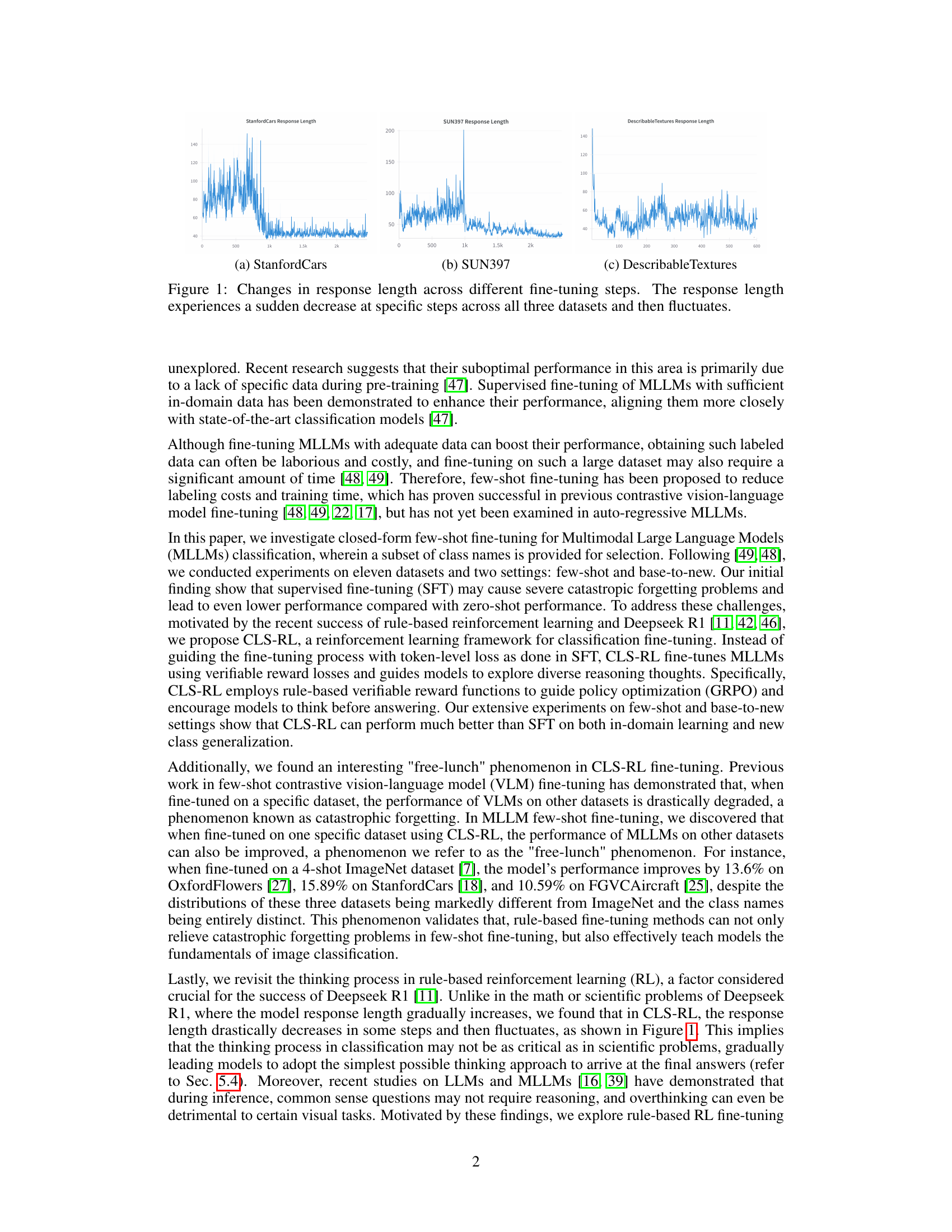
🔼 This figure visualizes the changes in the length of model responses generated during the fine-tuning process of three different datasets: StanfordCars, SUN397, and DescribableTextures. The x-axis represents the number of fine-tuning steps, while the y-axis shows the response length. The plot reveals that the response length is not consistently decreasing but instead undergoes sudden drops at certain points, followed by periods of fluctuation. This indicates that the model’s reasoning or ’thinking’ process isn’t linear during fine-tuning but instead involves abrupt shifts in its approach to the problem.
read the caption
Figure 1: Changes in response length across different fine-tuning steps. The response length experiences a sudden decrease at specific steps across all three datasets and then fluctuates.
| Base | New | H | |
|---|---|---|---|
| Qwen2VL | 62.1 | 66.27 | 64.12 |
| SFT | 67.4 | 70.73 | 69.03 |
| CLS-RL | 81.17 | 79.15 | 80.15 |
| no-thinking | 83.42 | 81.88 | 82.64 |
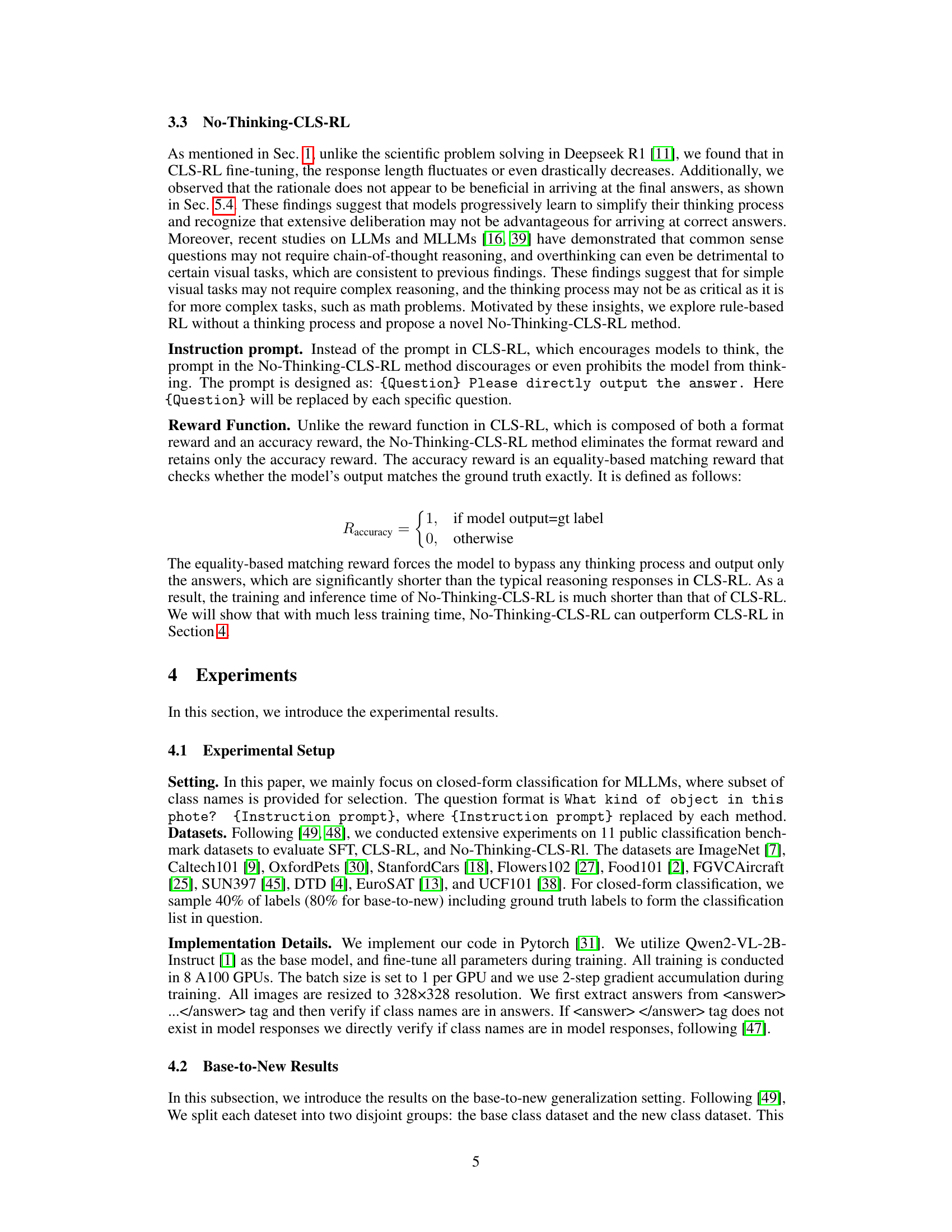
🔼 This table presents a comparison of four different methods for image classification fine-tuning on eleven benchmark datasets using the Qwen2VL instruction model. The methods compared are: the Qwen2VL instruct model without any fine-tuning, supervised fine-tuning (SFT), the proposed CLS-RL (Classification with Rule-based Reinforcement Learning) method, and a variation of CLS-RL called ‘No-Thinking-CLS-RL’. The evaluation is performed in a base-to-new generalization setting, meaning that a subset of classes is used for training (‘base classes’) and the performance is assessed on both the training classes and unseen classes (’new classes’). The table shows the accuracy achieved on ‘base’ classes and ’new’ classes for each method, and also presents the harmonic mean (H) of base and new class accuracies, providing a more comprehensive measure of generalization ability. ‘No-Thinking’ refers to the ‘No-Thinking-CLS-RL’ method.
read the caption
Table 1: Comparison of Qwen2VL instruct, SFT, CLS-RL, and no-thinking-RL in the base-to-new generalization setting. No-Thinking: no-thinking-RL. Base: base class accuracy. New: new class accuracy. H: harmonic mean accuracy. no-thinking: No-Thinking-CLS-RL.
In-depth insights#
RL & No Forgetting#
Reinforcement learning (RL) offers a promising avenue to combat catastrophic forgetting in multimodal models. Traditional fine-tuning often overwrites pre-existing knowledge, but RL, by optimizing for cumulative reward, can potentially retain broader capabilities. Rule-based RL, specifically, uses verifiable signals to guide learning, ensuring the model doesn’t stray too far from desired behaviors. This approach can mitigate forgetting by encouraging the model to leverage existing knowledge to achieve new tasks, rather than learning from scratch. Furthermore, the ‘free-lunch’ phenomenon observed with CLS-RL, where fine-tuning on one dataset improves performance on others, suggests a mechanism for knowledge consolidation and transfer, inherently reducing forgetting. By learning general classification principles, the model becomes more robust and less susceptible to performance degradation when faced with novel datasets.
CLS-RL vs. SFT#
CLS-RL demonstrates a significant advantage over SFT. CLS-RL achieves markedly higher accuracy, around 14%, for base classes and about 9% for new classes. Overall harmonic mean accuracy is 11% higher. CLS-RL is more effective in classification, showing rule-based reinforcement fine-tuning is useful. The results indicate that for image classification, CLS-RL framework surpasses the SFT framework because it can take advantage of more context and reasoning during the training process. It can fine-tune the parameters much more accurately and effectively.
No-Think > Think?#
The paper challenges the conventional wisdom that complex reasoning is always beneficial in multimodal tasks. The core concept, ‘No-Think > Think?’, suggests that for some visual classification problems, reducing the cognitive load and encouraging direct answer generation can outperform methods that promote extensive reasoning. This is counterintuitive, as many recent advances in large language models (LLMs) emphasize chain-of-thought reasoning. The key findings are that a simpler approach, where the model directly outputs the answer, can lead to better accuracy and efficiency. This implies that the nature of the task plays a crucial role. Complex reasoning might be necessary for tasks requiring multi-step inference, but can be detrimental when it introduces unnecessary noise or complexity for simpler classifications. Also, ’thinking process’ in fine-tuning might not be that important, or even detrimental, for simple visual tasks such as classification. Moreover, by compelling the model to only output the answer, the training time is significantly shorter. This challenges the assumption that explicit reasoning steps are always beneficial for visual tasks, and underscores the importance of task-specific adaptation in MLLMs.
Free-Lunch Effect#
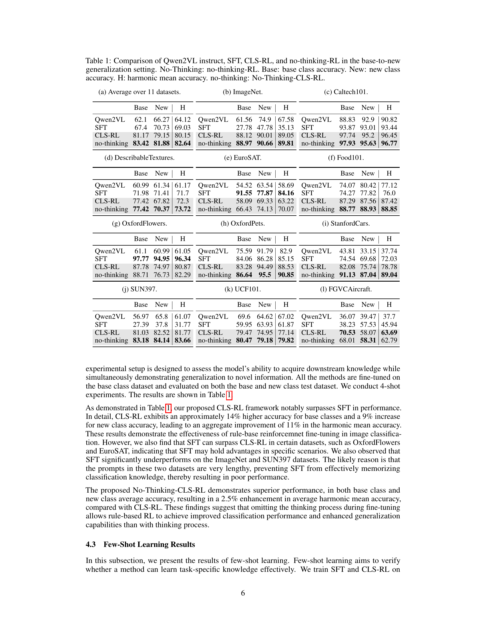
The “free-lunch” effect in the context of MLLM fine-tuning, particularly with CLS-RL, presents a fascinating phenomenon. Unlike contrastive VLMs where fine-tuning on one dataset often leads to catastrophic forgetting on others, CLS-RL can sometimes improve performance across diverse datasets. This suggests that instead of merely memorizing dataset-specific information, the RL-based fine-tuning is enabling the model to learn more generalizable visual concepts or classification strategies. This implies that CLS-RL is genuinely teaching fundamental aspects of image classification to the model. The fact that improvements occur even with datasets differing significantly in distribution and class names supports this claim. However, the effect isn’t universally positive; some datasets may see diminished performance after fine-tuning on others, hinting at potential interference or concept divergence. Further exploration into the factors influencing this ‘free-lunch’ effect, such as dataset similarity or the nature of the learned representations, would be valuable. The contrast between the ‘free-lunch’ effect and catastrophic forgetting further validates the RL-based method.
Dataset Limits#
While the research paper extensively explores image classification with rule-based reinforcement learning (CLS-RL), it’s crucial to acknowledge dataset limitations. The reliance on specific, curated datasets might hinder the generalizability of findings to real-world scenarios with diverse or noisy data. The paper mentions experiments on eleven public datasets, there could be a bias towards well-defined categories and clean images, potentially overestimating the performance of CLS-RL in more ambiguous settings. Furthermore, the limited size of few-shot learning datasets raises questions about the robustness of the learned models and their ability to handle unseen variations within a class. The ‘free-lunch’ phenomenon, where fine-tuning on one dataset improves performance on others, also needs careful scrutiny. The datasets used in this context should be further researched to discover potential overlapping between datasets, and any biases introduced by them. It’s essential to investigate how CLS-RL performs on datasets with varying levels of difficulty and distributional shifts to gain a more comprehensive understanding of its capabilities. Additionally, the paper should address the potential for overfitting to the specific characteristics of the datasets used, and explore techniques for mitigating this risk. Analyzing performance across a wider range of datasets with varying properties is vital for assessing the true potential and limitations of CLS-RL.
More visual insights#
More on tables
| Base | New | H | |
|---|---|---|---|
| Qwen2VL | 61.56 | 74.9 | 67.58 |
| SFT | 27.78 | 47.78 | 35.13 |
| CLS-RL | 88.12 | 90.01 | 89.05 |
| no-thinking | 88.97 | 90.66 | 89.81 |
🔼 This table presents a comparison of the performance of four different methods: Qwen2VL instruct (a baseline), Supervised Fine-Tuning (SFT), CLS-RL, and No-Thinking-CLS-RL on eleven image classification datasets. The comparison is done in a base-to-new generalization setting, where the models are initially trained on a subset of classes (‘base’) and then evaluated on those classes and a set of unseen classes (’new’). The table shows the ‘base’ and ’new’ classification accuracies, as well as the harmonic mean of these two metrics (H), providing a comprehensive evaluation across different model approaches and dataset splits. The average performance across all eleven datasets is also summarized.
read the caption
(a) Average over 11 datasets.
| Base | New | H | |
|---|---|---|---|
| Qwen2VL | 88.83 | 92.9 | 90.82 |
| SFT | 93.87 | 93.01 | 93.44 |
| CLS-RL | 97.74 | 95.2 | 96.45 |
| no-thinking | 97.93 | 95.63 | 96.77 |
🔼 This table presents a comparison of the performance of different methods on the ImageNet dataset in the base-to-new generalization setting. It shows the base class accuracy (accuracy on classes present in both training and testing sets), new class accuracy (accuracy on classes only present in the testing set), and the harmonic mean of these two accuracies. The methods compared are Qwen2VL (a baseline model), supervised fine-tuning (SFT), CLS-RL, and No-Thinking-CLS-RL. The results illustrate the relative effectiveness of each method in generalizing to unseen classes.
read the caption
(b) ImageNet.
| Base | New | H | |
|---|---|---|---|
| Qwen2VL | 60.99 | 61.34 | 61.17 |
| SFT | 71.98 | 71.41 | 71.7 |
| CLS-RL | 77.42 | 67.82 | 72.3 |
| no-thinking | 77.42 | 70.37 | 73.72 |
🔼 This table presents a comparison of the performance of four different methods on the Caltech101 dataset in a base-to-new generalization setting. It shows base class accuracy, new class accuracy, and harmonic mean accuracy for each method: Qwen2VL, Supervised Fine-Tuning (SFT), CLS-RL, and No-Thinking-CLS-RL. The results illustrate the performance differences between these approaches in adapting to unseen data.
read the caption
(c) Caltech101.
| Base | New | H | |
|---|---|---|---|
| Qwen2VL | 54.52 | 63.54 | 58.69 |
| SFT | 91.55 | 77.87 | 84.16 |
| CLS-RL | 58.09 | 69.33 | 63.22 |
| no-thinking | 66.43 | 74.13 | 70.07 |
🔼 This table presents a comparison of the performance of different methods on the Describable Textures dataset in a base-to-new generalization setting. It shows the base class accuracy (accuracy on classes present in both training and testing sets), the new class accuracy (accuracy on classes only in the testing set), and the harmonic mean of these two accuracies for four different methods: Qwen2VL (a baseline), SFT (supervised fine-tuning), CLS-RL (the proposed method), and No-Thinking-CLS-RL (a variant of CLS-RL). This allows for a comparison of the models’ ability to generalize to unseen classes and their overall performance on this specific dataset.
read the caption
(d) DescribableTextures.
| Base | New | H | |
|---|---|---|---|
| Qwen2VL | 74.07 | 80.42 | 77.12 |
| SFT | 74.27 | 77.82 | 76.0 |
| CLS-RL | 87.29 | 87.56 | 87.42 |
| no-thinking | 88.77 | 88.93 | 88.85 |
🔼 Table 1 presents a comparison of the performance of different image classification methods on the EuroSAT dataset in a base-to-new generalization setting. It shows the base class accuracy (accuracy on classes seen during training), new class accuracy (accuracy on unseen classes), and the harmonic mean of these two metrics for each method. The methods compared include Qwen2VL (a baseline model), Supervised Fine-Tuning (SFT), CLS-RL (the proposed method), and No-Thinking-CLS-RL (a variation of the proposed method). This allows for a detailed assessment of how each method generalizes to new classes after fine-tuning on the EuroSAT dataset.
read the caption
(e) EuroSAT.
| Base | New | H | |
|---|---|---|---|
| Qwen2VL | 61.1 | 60.99 | 61.05 |
| SFT | 97.77 | 94.95 | 96.34 |
| CLS-RL | 87.78 | 74.97 | 80.87 |
| no-thinking | 88.71 | 76.73 | 82.29 |
🔼 This table presents a comparison of the performance of different image classification methods on the Food101 dataset. The methods compared are Qwen2VL (a baseline model), Supervised Fine-Tuning (SFT), CLS-RL (the proposed rule-based reinforcement learning method), and No-Thinking-CLS-RL (a variant of CLS-RL). The performance is evaluated in a base-to-new setting, measuring the accuracy on both base classes (used for fine-tuning) and new classes (not seen during fine-tuning). The harmonic mean of base and new class accuracies (H) is also provided as a combined performance metric. This allows for a comprehensive comparison of the effectiveness of these methods in both in-domain and out-of-domain image classification scenarios.
read the caption
(f) Food101.
| Base | New | H | |
|---|---|---|---|
| Qwen2VL | 75.59 | 91.79 | 82.9 |
| SFT | 84.06 | 86.28 | 85.15 |
| CLS-RL | 83.28 | 94.49 | 88.53 |
| no-thinking | 86.64 | 95.5 | 90.85 |
🔼 This table presents a comparison of the performance of four different methods on the OxfordFlowers dataset in a base-to-new generalization setting. The methods compared are: Qwen2VL (a baseline zero-shot model), Supervised Fine-Tuning (SFT), CLS-RL (the proposed rule-based reinforcement learning method), and No-Thinking-CLS-RL (a variation of CLS-RL minimizing the ’thinking’ process). The table shows the accuracy achieved by each method on base classes (classes present in the training data) and new classes (classes not seen during training), along with the harmonic mean of these accuracies. This allows for evaluation of the model’s ability to generalize to unseen data.
read the caption
(g) OxfordFlowers.
| Base | New | H | |
|---|---|---|---|
| Qwen2VL | 43.81 | 33.15 | 37.74 |
| SFT | 74.54 | 69.68 | 72.03 |
| CLS-RL | 82.08 | 75.74 | 78.78 |
| no-thinking | 91.13 | 87.04 | 89.04 |
🔼 This table presents a comparison of the performance of four different methods (Qwen2VL instruct, SFT, CLS-RL, and No-Thinking-CLS-RL) on the OxfordPets dataset in a base-to-new generalization setting. It shows the accuracy achieved by each method on both the base class (already seen during training) and new class (unseen during training). The ‘H’ column represents the harmonic mean of base and new class accuracies, providing a balanced view of the model’s overall performance. This allows for a comprehensive evaluation of how well each method generalizes to novel data, reflecting its ability to learn generalizable image classification knowledge rather than simply memorizing training examples.
read the caption
(h) OxfordPets.
| Base | New | H | |
|---|---|---|---|
| Qwen2VL | 56.97 | 65.8 | 61.07 |
| SFT | 27.39 | 37.8 | 31.77 |
| CLS-RL | 81.03 | 82.52 | 81.77 |
| no-thinking | 83.18 | 84.14 | 83.66 |
🔼 Table 1 presents a comparison of four different methods for image classification: Qwen2VL instruct (a baseline), Supervised Fine-tuning (SFT), CLS-RL, and No-Thinking-CLS-RL. The comparison is done across eleven datasets, evaluating performance in two distinct settings: ‘base-to-new’ (where the model is trained on a subset of classes and tested on both seen and unseen classes) and ‘few-shot’ (where the model is trained on very limited data per class). For each dataset and method, the table shows the classification accuracy on the base classes, new classes, and the harmonic mean of these two accuracies. The table allows a direct comparison of the effectiveness of the different methods in terms of both in-domain and out-of-domain generalization.
read the caption
(i) StanfordCars.
| Base | New | H | |
|---|---|---|---|
| Qwen2VL | 69.6 | 64.62 | 67.02 |
| SFT | 59.95 | 63.93 | 61.87 |
| CLS-RL | 79.47 | 74.95 | 77.14 |
| no-thinking | 80.47 | 79.18 | 79.82 |
🔼 The table presents a comparison of different methods for image classification on the SUN397 dataset. It shows the performance (base class accuracy, new class accuracy, and harmonic mean accuracy) of Qwen2VL instruct, supervised fine-tuning (SFT), CLS-RL, and No-Thinking-CLS-RL in a base-to-new generalization setting. This allows for assessment of how well each method generalizes from a set of base classes to unseen new classes.
read the caption
(j) SUN397.
| Base | New | H | |
|---|---|---|---|
| Qwen2VL | 36.07 | 39.47 | 37.7 |
| SFT | 38.23 | 57.53 | 45.94 |
| CLS-RL | 70.53 | 58.07 | 63.69 |
| no-thinking | 68.01 | 58.31 | 62.79 |
🔼 Table 1 presents a comparison of four different methods for image classification using the Qwen2VL-Instruct model: Qwen2VL, Supervised Fine-Tuning (SFT), CLS-RL (Classification with Rule-Based Reinforcement Learning), and No-Thinking-CLS-RL. The table displays the performance metrics (Base class accuracy, New class accuracy, and Harmonic mean accuracy) across eleven datasets. The ‘Base-to-New’ experimental setting is used, where models are trained on a subset of classes and tested on both seen (base) and unseen (new) classes. This allows for the evaluation of generalization capabilities. Each row represents a different model and method, allowing comparison across these techniques.
read the caption
(k) UCF101.
ImageNet | Caltech101 | DTD | EuroSAT | Food101 | Flowers102 | OxfordPets | S.C. | SUN397 | UCF101 | F.A. | Average | |
|---|---|---|---|---|---|---|---|---|---|---|---|---|
| Qwen2VL | 70.8 | 88.56 | 54.79 | 45.68 | 77.54 | 64.43 | 73.89 | 35.77 | 63.83 | 66.22 | 42.75 | 62.21 |
| SFT | 41.60 | 93.91 | 71.336 | 75.16 | 75.75 | 96.87 | 85.80 | 71.13 | 41.66 | 63.81 | 60.15 | 70.65 |
| CLS-RL | 92.24 | 98.09 | 69.92 | 49.46 | 88.94 | 86.56 | 87.24 | 80.24 | 84.57 | 82.1 | 74.41 | 81.25 |
| No-Thinking-RL | 92.31 | 98.46 | 73.52 | 58.02 | 90.78 | 91.6 | 86.13 | 92.5 | 86.72 | 83.82 | 74.41 | 84.39 |
🔼 Table 1 presents a comparison of the performance of four different methods on eleven image classification datasets. The methods compared are Qwen2VL instruct (a baseline), Supervised Fine-Tuning (SFT), CLS-RL, and No-Thinking-CLS-RL. The table shows the accuracy achieved by each method on the base classes (classes used for fine-tuning) and new classes (unseen classes) for each of the datasets. The harmonic mean of base and new class accuracies is also provided to summarize overall performance. The results are displayed for both few-shot and base-to-new settings. The purpose is to show the effectiveness of the CLS-RL and No-Thinking-CLS-RL methods in comparison to supervised fine-tuning in few-shot and base-to-new image classification scenarios.
read the caption
(l) FGVCAircraft.
| Accuracy | Training Time | Inference Time | |
|---|---|---|---|
| SFT | 41.60 | 35 min | 20min |
| CLS-RL | 92.24 | 1587 min | 30 min |
| No-Thinking-CLS-RL | 92.31 | 94 min | 26 min |
🔼 This table presents the results of few-shot learning experiments conducted on eleven image classification datasets. For each dataset, it shows the accuracy achieved by the baseline Qwen2VL model, a supervised fine-tuning (SFT) approach, a rule-based reinforcement learning method (CLS-RL), and a modified version of CLS-RL that minimizes the ’thinking process’ (No-Thinking-CLS-RL). The results are broken down for StanfordCars and FGVCAircraft datasets, and an average across all eleven datasets is provided for comparison. The table showcases the performance of each method under a limited-data setting.
read the caption
Table 2: Few-shot learning results. S.C.: StanfordCars dataset. F.A.: FGVCAircraft dataset.
| ImageNet | Caltech101 | Food101 | Flowers102 | OxfordPets | Average | |
|---|---|---|---|---|---|---|
| Qwen2VL | 46.57 | 62.96 | 57.79 | 48.44 | 47.40 | 52.63 |
| CLS-RL | 54.84 | 79.07 | 73.51 | 67.64 | 89.94 | 73.0 |
| No-Thinking-CLS-RL | 56.45 | 86.29 | 71.99 | 71.21 | 86.07 | 74.40 |
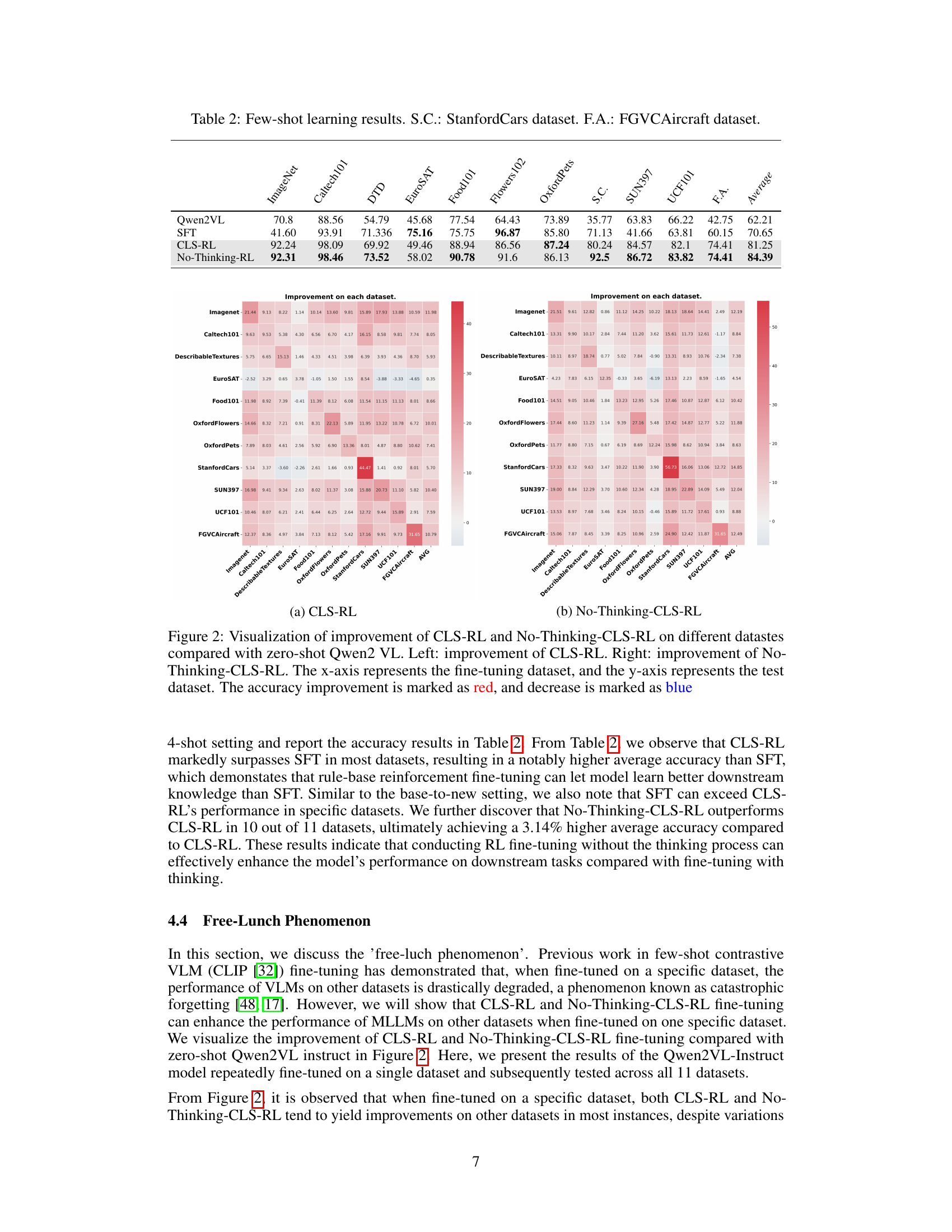
🔼 This table compares the training time and inference time, in minutes, for the CLS-RL and No-Thinking-CLS-RL models, in addition to their accuracy. It demonstrates the significant efficiency gains achieved by No-Thinking-CLS-RL due to its simplified training process.
read the caption
Table 3: Training and inference efficiency comparison between CLS-RL and No-Thinking-CLS-RL.
Full paper#