TL;DR#
3D shape generation has advanced rapidly with Vecset Diffusion Models (VDMs), but high-speed generation remains a challenge. VDMs struggle due to slow diffusion sampling and Variational Autoencoder (VAE) decoding. Existing methods for image acceleration are not suitable for VDM because of the different nature of the 3D meshes and latent spaces. Therefore, improving VDM speed is crucial for interactive applications.
This paper presents FlashVDM, a framework that accelerates both VAE and diffusion processes in VDMs. For diffusion acceleration, it uses Progressive Flow Distillation, achieving high-quality results with as few as 5 inference steps. For VAE acceleration, it introduces a lightning vecset decoder with Adaptive KV Selection and Hierarchical Volume Decoding. This design lowers FLOPs and decoding overhead, achieving over 45x speedup in VAE decoding and 32x speedup overall.
Key Takeaways#
Why does it matter?#
This paper introduces FlashVDM, achieving over 32x speedup in 3D shape generation while maintaining fidelity. It is a significant advancement towards real-time 3D content creation, offering new avenues for interactive design and AI-driven content generation tools. Its impact is in faster prototyping and democratizing 3D design.
Visual Insights#

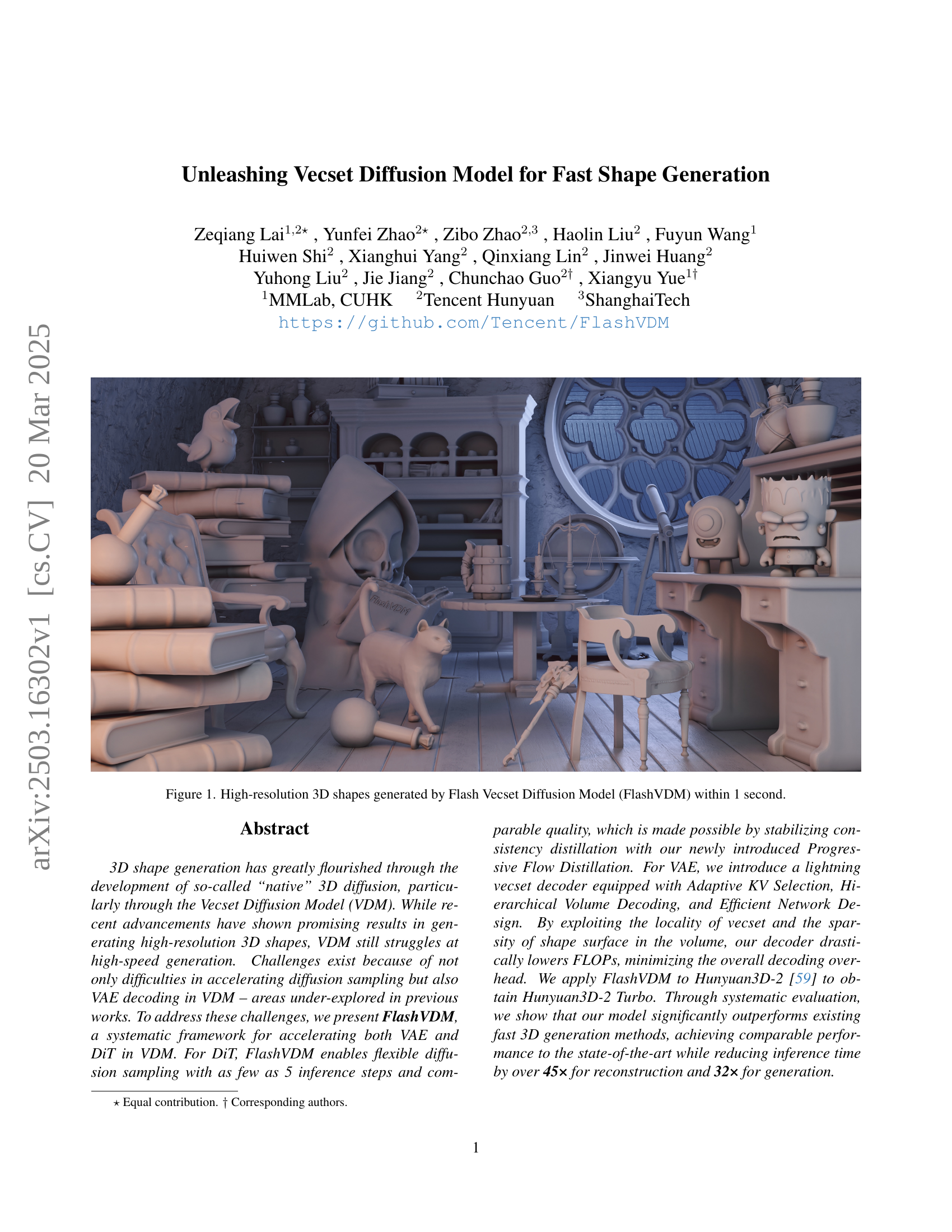
🔼 This figure showcases examples of high-resolution 3D shapes generated using the Flash Vecset Diffusion Model (FlashVDM). It highlights the model’s ability to produce detailed and complex 3D models in just one second, demonstrating its speed and effectiveness. The variety of objects depicted in the image, ranging from animals and common household objects to more fantastical items, illustrates the breadth of the model’s generative capabilities.
read the caption
Figure 1: High-resolution 3D shapes generated by Flash Vecset Diffusion Model (FlashVDM) within 1 second.
| V-IoU() | S-IoU() | Time(s) | |
| 3DShape2VecSet [54] | 87.88% | 84.93% | 16.43 |
| Michelangelo [58] | 84.93% | 76.27% | 16.43 |
| Direct3D [45] | 88.43% | 81.55% | 3.201 |
| Hunyuan3D-2 [59]-1024 | 93.60% | 89.16% | 16.43 |
| with FlashVDM | 91.90% | 88.02% | 0.382 |
| Hunyuan3D-2 [59]-3072 | 96.11% | 93.27% | 22.33 |
| with FlashVDM | 95.55% | 93.10% | 0.491 |
🔼 This table presents a quantitative comparison of several methods for 3D shape reconstruction. It compares the performance of different methods including 3DShape2VecSet, Michelangelo, Direct3D, and the proposed method (Hunyuan3D-2 with FlashVDM) across two different resolutions (1024 and 3072). The metrics used for comparison are Volume IoU (V-IoU), Surface IoU (S-IoU), and the reconstruction time. Higher V-IoU and S-IoU values indicate better reconstruction accuracy, while lower reconstruction time implies faster performance. The table aims to demonstrate the improvement in speed and accuracy achieved by the proposed approach.
read the caption
Table 1: Numerical comparisons of shape reconstruction methods.
In-depth insights#
VDM Bottleneck#
The VDM architecture, while powerful, introduces bottlenecks. A primary bottleneck lies in the computational intensity of the VAE decoder, particularly its cross-attention mechanism. Decoding shape latents into a high-resolution SDF volume requires numerous queries, scaling cubically with resolution. The large number of key-value pairs further exacerbates this. This contrasts sharply with image diffusion models, where decoding is less demanding. Consequently, VAE decoding in VDM consumes a significant portion of inference time, often exceeding diffusion sampling itself. Techniques like progressive flow distillation and VAE acceleration are crucial to alleviate these bottlenecks. Effective acceleration strategies include reducing queries (hierarchical decoding), minimizing key-value pairs (adaptive KV selection), and optimizing decoder architecture to enhance overall efficiency.
Progressive Distill#
Progressive distillation is a multi-stage approach to training efficient models, particularly in generative tasks. It involves gradually transferring knowledge from a larger, pre-trained model (the teacher) to a smaller, faster model (the student). The process starts with a simpler form of distillation, such as guidance distillation, to stabilize the student model before introducing more complex distillation techniques. This initial phase helps the student learn the overall structure and distribution of the data. Subsequent stages involve more advanced distillation methods, like consistency distillation, which enforces the student model to produce consistent outputs across different sampling steps or time points. The progressive nature of this approach allows the student to learn the complex relationships in the data without becoming unstable or overfitting early on. Additional techniques, such as adversarial finetuning, may be incorporated to further refine the student model and improve its output quality. Progressive distillation enables a significant reduction in inference time while maintaining high fidelity outputs.
Hierarchical VAE#
While not explicitly a heading in this paper, a hierarchical VAE structure suggests a multi-scale approach to encoding and decoding 3D shapes, aligning with the paper’s focus on accelerating VAEs in the context of 3D diffusion models. The core idea would be to represent the 3D shape at varying levels of detail, possibly using a coarse-to-fine strategy. The encoder could progressively downsample the input (e.g., point cloud or volume), extracting features at each level, while the decoder would reconstruct the shape in a hierarchical manner, starting with a low-resolution approximation and progressively adding finer details. This approach aligns well with sparsity of shape surface, as only regions near the surface need high-resolution decoding. This can be used to adaptively refine areas of interest, potentially leading to significant computational savings and improved quality compared to dense decoding. It aligns with octree decoding and Adaptive KV Selection to minimize FLOPs.
45x Faster Decode#
The term “45x Faster Decode” implies a significant optimization in the decoding process, likely within a machine learning or data processing context. This level of speedup suggests a complete overhaul or highly efficient redesign of the decoding algorithm or hardware. The acceleration might stem from techniques like parallel processing, algorithm optimization, or hardware acceleration, resulting in a substantial reduction in processing time. This advancement likely addresses a crucial bottleneck, enabling faster overall system performance, particularly in real-time applications. Faster decoding improves efficiency, reduces latency, and enhances user experience. This level of improvement may be impactful in a lot of cases, it signifies a pivotal development in its respective area. The method may use efficient cache utilization, reduced memory accesses, or optimized branching strategies. Furthermore, this faster decoding could be crucial for models deployed on resource-constrained devices, making complex models more accessible and practical. Therefore, a 45x speedup in decoding demonstrates a significant technological achievement.
Turbo 3D Models#
Turbo 3D Models represents a crucial advancement in efficient 3D content generation, addressing the ever-present need for speed without sacrificing quality. The core idea revolves around techniques that dramatically accelerate the creation of 3D models, potentially through model distillation, optimized architectures, or novel training strategies. A key goal is to reduce the computational cost associated with 3D model generation, enabling real-time or near real-time applications. This could involve reducing inference time, memory footprint, or energy consumption. Such models are highly desirable for applications like interactive design, virtual reality, and rapid prototyping where speed is paramount. Challenges include maintaining high fidelity and geometric accuracy while achieving significant speedups and ensuring that Turbo models retain the expressive power of their slower counterparts.
More visual insights#
More on figures

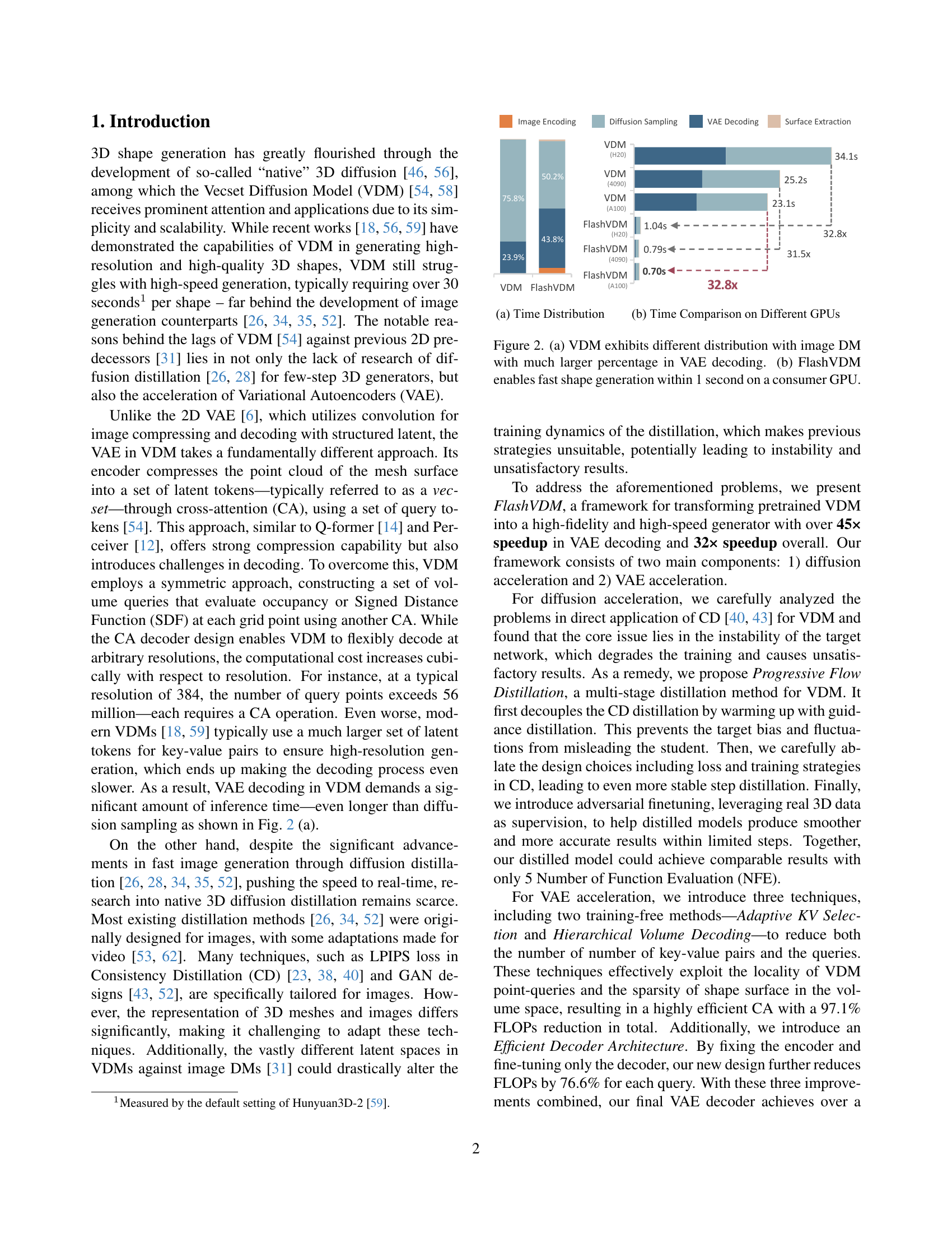
🔼 Figure 2(a) compares the time distribution of different processing stages in a Vecset Diffusion Model (VDM) and an image diffusion model. It highlights that VDM spends a significantly larger proportion of its time on Variational Autoencoder (VAE) decoding compared to other stages like diffusion sampling or surface extraction. Figure 2(b) demonstrates the speed improvement achieved by FlashVDM. It shows that FlashVDM can generate a high-resolution 3D shape in under a second on a standard consumer GPU, representing a substantial speedup compared to the original VDM.
read the caption
Figure 2: (a) VDM exhibits different distribution with image DM with much larger percentage in VAE decoding. (b) FlashVDM enables fast shape generation within 1 second on a consumer GPU.

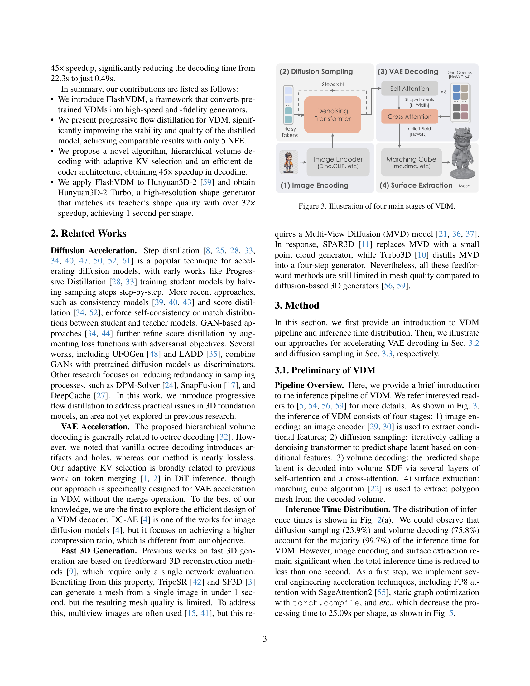
🔼 This figure illustrates the four main stages of the Vecset Diffusion Model (VDM) pipeline for 3D shape generation. It starts with (1) image encoding, where an image encoder processes an input image to extract conditional features. These features are then used in (2) diffusion sampling, an iterative process of denoising shape latents using a denoising transformer. The resulting shape latents are then passed to (3) VAE decoding, which uses self and cross-attention mechanisms to decode the latents into a 3D volume representation (SDF). Finally, (4) surface extraction employs a method like marching cubes to convert the volume representation into a polygon mesh.
read the caption
Figure 3: Illustration of four main stages of VDM.

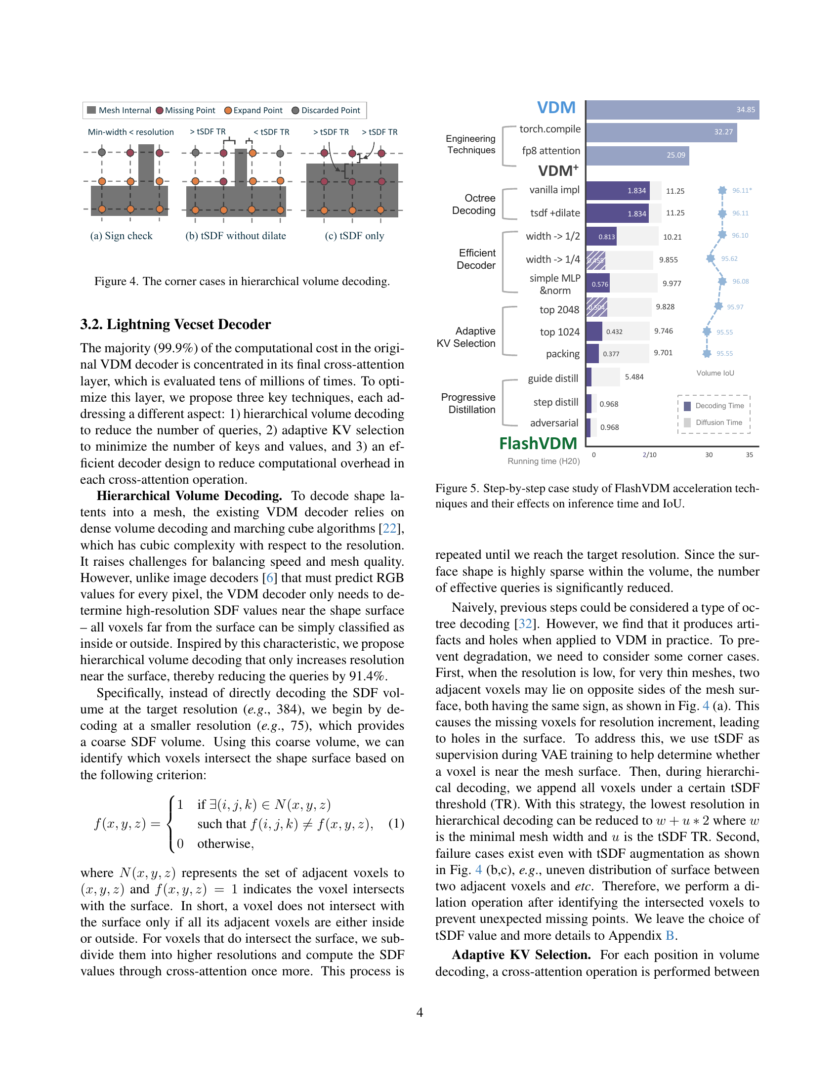
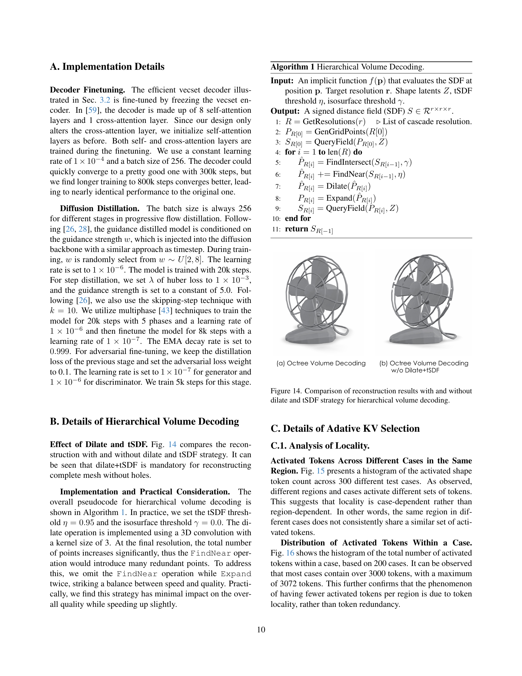
🔼 This figure illustrates three scenarios where the hierarchical volume decoding method used in the Lightning Vecset Decoder might fail to produce a complete mesh. It highlights the challenges in reconstructing thin meshes at low resolutions due to the limitations of using the sign of the SDF values (Signed Distance Function). The three cases illustrate how simple voxel-level considerations can lead to missing parts of the mesh during the decoding process, necessitating additional techniques (like dilation and tSDF thresholds) to improve results.
read the caption
Figure 4: The corner cases in hierarchical volume decoding.

🔼 Figure 5 shows a step-by-step breakdown of how each acceleration technique implemented in FlashVDM affects both inference time and Intersection over Union (IoU). It starts with the baseline VDM performance, then progressively introduces: (1) engineering optimizations (like FP8 attention and graph compilation), (2) hierarchical volume decoding in the decoder, (3) adaptive Key-Value (KV) selection, (4) an efficient decoder architecture, and finally (5) progressive flow distillation. For each step, the figure displays the resulting inference time and IoU, illustrating how the cumulative effects of these techniques significantly improve efficiency without substantially sacrificing accuracy.
read the caption
Figure 5: Step-by-step case study of FlashVDM acceleration techniques and their effects on inference time and IoU.

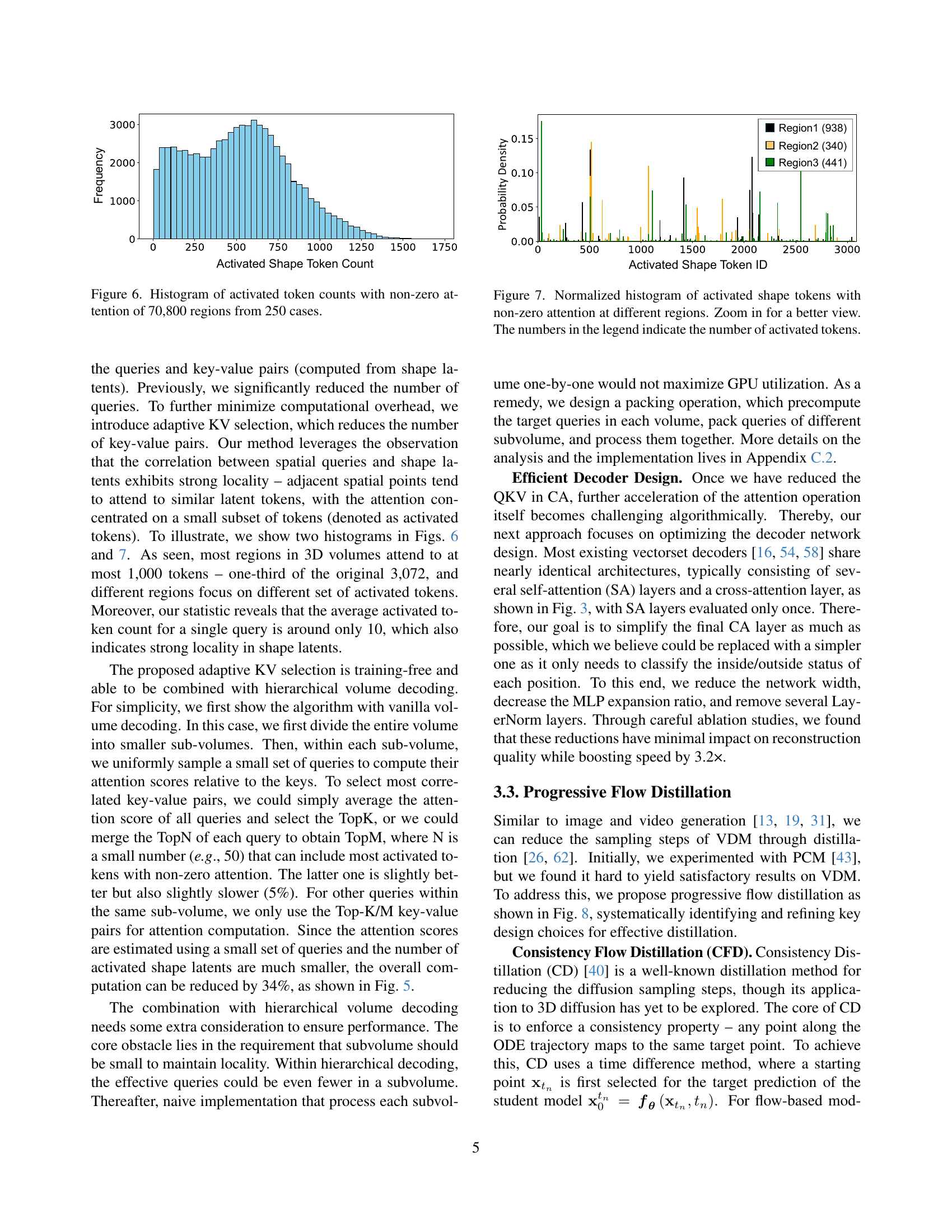
🔼 This histogram visualizes the distribution of activated token counts across 70,800 regions derived from 250 different cases. Each bar represents a specific token count, and the height of the bar indicates how many regions exhibited that count of activated tokens. This data illustrates the concept of locality, showing that only a subset of available tokens is activated within each region, and those tokens are frequently similar in neighboring regions. This is particularly important for the efficiency of the adaptive KV selection method described in the paper.
read the caption
Figure 6: Histogram of activated token counts with non-zero attention of 70,800 regions from 250 cases.

🔼 This figure presents normalized histograms visualizing the distribution of activated shape tokens across three different regions within a 3D volume. Each histogram shows the frequency of tokens with non-zero attention, indicating the number of shape tokens that each spatial query attends to. The x-axis represents the activated shape token ID, and the y-axis represents the normalized frequency. The numbers within the legend represent the count of activated tokens in each region, offering insight into the sparsity and locality of attention within the 3D shape generation process. Zooming in reveals finer details in the distribution of activated tokens.
read the caption
Figure 7: Normalized histogram of activated shape tokens with non-zero attention at different regions. Zoom in for a better view. The numbers in the legend indicate the number of activated tokens.

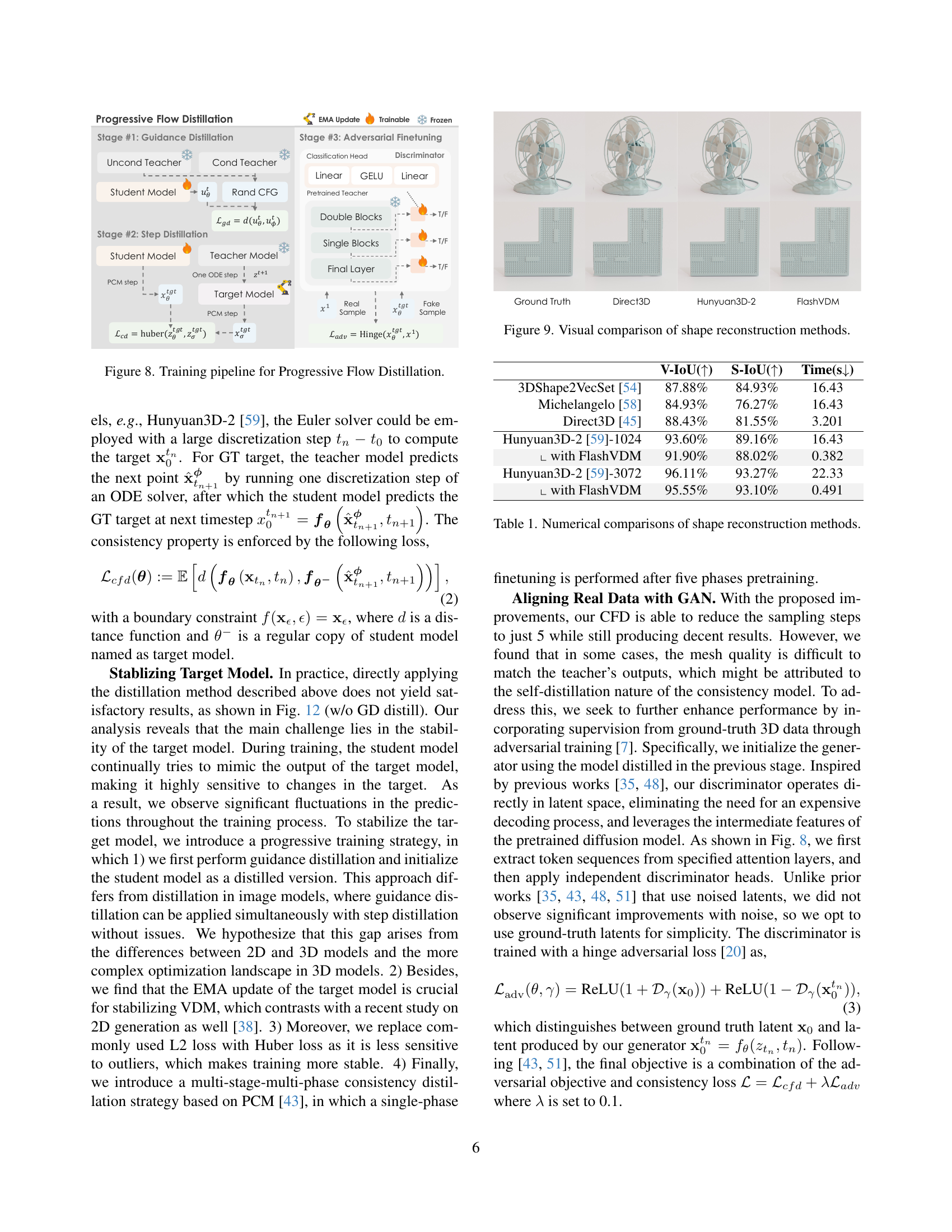
🔼 This figure details the training pipeline for the Progressive Flow Distillation method used to accelerate diffusion sampling in the Vecset Diffusion Model. It shows a three-stage process: 1) Guidance Distillation, where the student model is initialized using a teacher model. 2) Step Distillation, involving iterative training of the student to match the teacher’s performance over fewer steps. 3) Adversarial Fine-tuning, where real 3D data is used to refine the student model’s accuracy. Each stage uses specific loss functions and training techniques to ensure stability and high-fidelity output.
read the caption
Figure 8: Training pipeline for Progressive Flow Distillation.

🔼 Figure 9 presents a visual comparison of the shape reconstruction results from several methods: Michelangelo, 3DShape2VecSet, Direct3D, and FlashVDM. It allows for a qualitative assessment of each method’s reconstruction capabilities, highlighting differences in detail preservation, surface smoothness, and overall shape accuracy.
read the caption
Figure 9: Visual comparison of shape reconstruction methods.

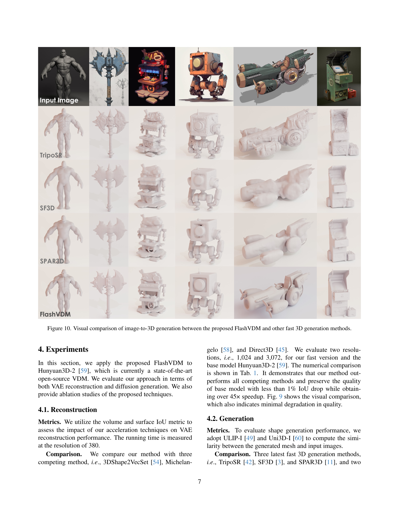
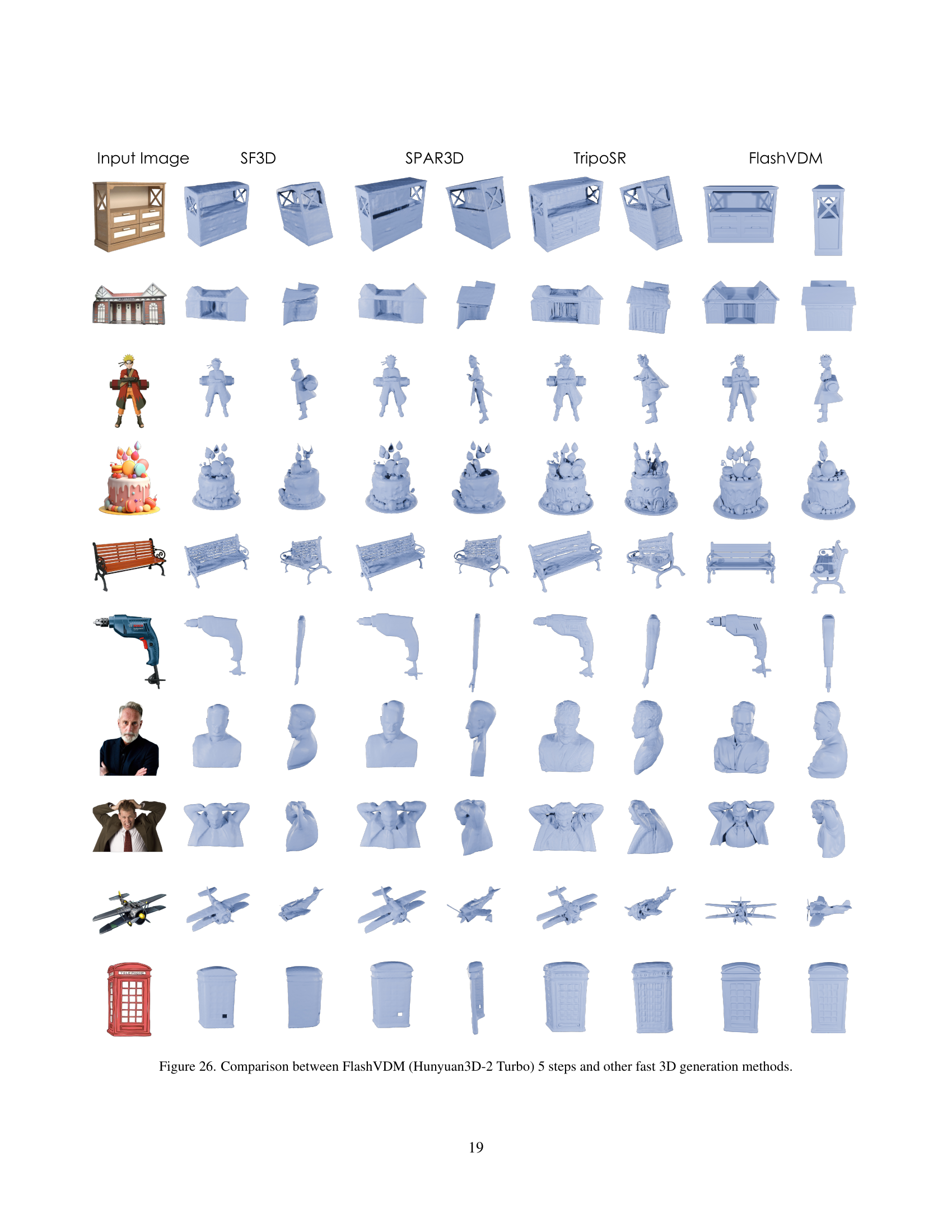
🔼 This figure compares the 3D model generation results of four different methods: TripoSR, SF3D, SPAR3D, and the proposed FlashVDM. Each method was given the same input image and tasked with generating a corresponding 3D model. The visual comparison showcases the differences in quality and detail achieved by each method, highlighting the superior performance of FlashVDM.
read the caption
Figure 10: Visual comparison of image-to-3D generation between the proposed FlashVDM and other fast 3D generation methods.

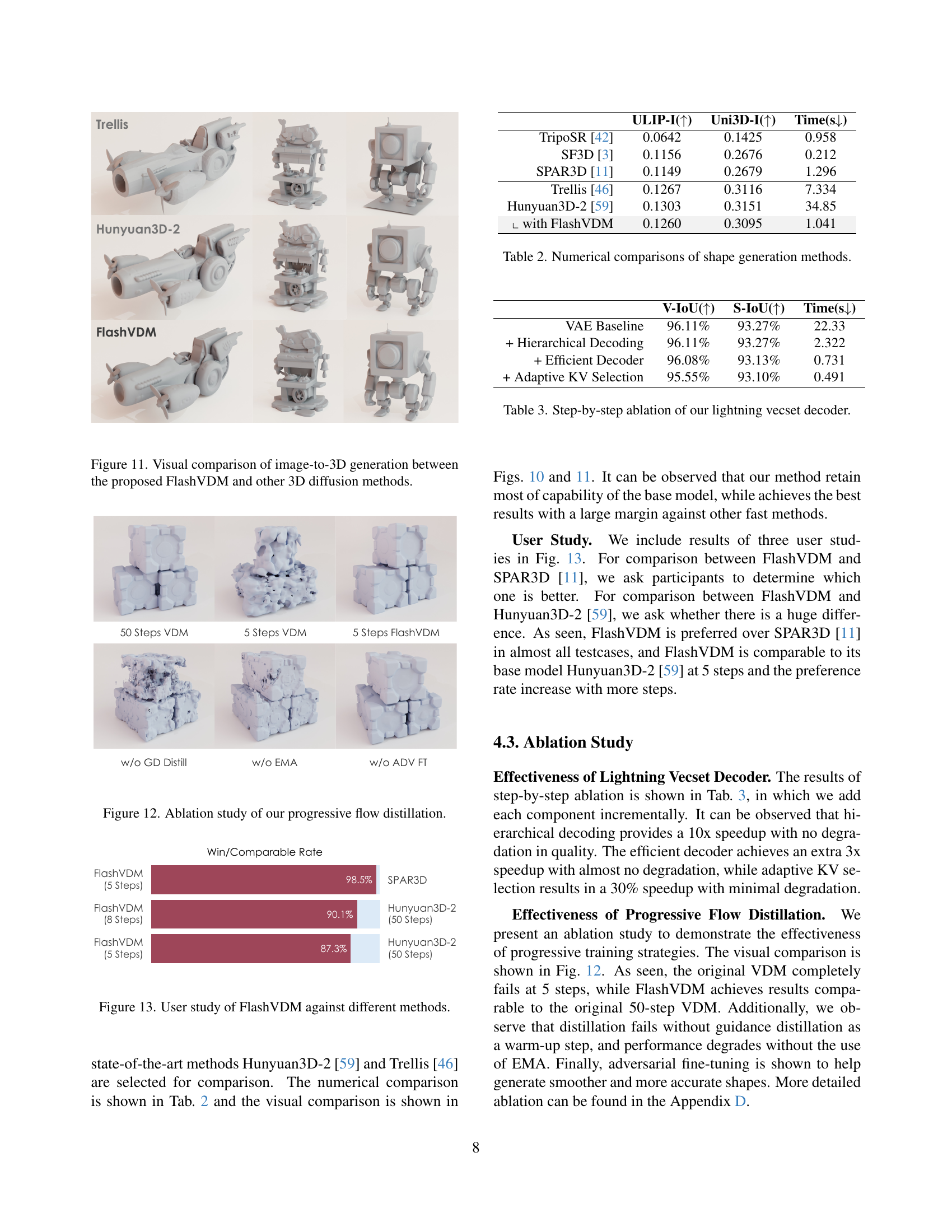
🔼 This figure provides a visual comparison of 3D model generation results from different methods, namely FlashVDM (the proposed method) and other state-of-the-art 3D diffusion models. It showcases various image prompts and their corresponding 3D model outputs, allowing a direct visual comparison of the mesh quality and detail generated by each method. The goal is to demonstrate the superiority of FlashVDM in terms of both accuracy and speed of 3D model generation.
read the caption
Figure 11: Visual comparison of image-to-3D generation between the proposed FlashVDM and other 3D diffusion methods.

🔼 This ablation study visualizes the effects of each stage in the proposed progressive flow distillation method on the quality of 3D model generation. It compares the results of using the full progressive flow distillation method to versions omitting guidance distillation, EMA updates, and adversarial finetuning. The figure demonstrates the importance of each component for achieving high-quality results even with a limited number of diffusion steps.
read the caption
Figure 12: Ablation study of our progressive flow distillation.

🔼 This figure presents the results of a user study comparing the performance of FlashVDM against other state-of-the-art 3D shape generation methods, namely Hunyuan3D-2 (50 steps) and Trellis. The user study aimed to evaluate the relative quality of shapes generated by FlashVDM (with 5 and 8 sampling steps) compared to the other methods. The win/comparable rate represents the percentage of times users preferred FlashVDM over other methods.
read the caption
Figure 13: User study of FlashVDM against different methods.

🔼 This figure compares the 3D reconstruction results obtained using the hierarchical volume decoding method with and without two key techniques: dilation and signed distance function (tSDF). Hierarchical volume decoding aims to improve efficiency by focusing computational resources on areas near the shape’s surface. Dilation is a morphological operation that expands the boundaries of a shape, while tSDF provides information about the distance from each point to the closest point on the shape’s surface. The figure visually illustrates how these techniques help in creating more complete and accurate 3D mesh reconstructions by addressing issues like holes in the mesh surface, particularly when dealing with thin objects.
read the caption
Figure 14: Comparison of reconstruction results with and without dilate and tSDF strategy for hierarchical volume decoding.

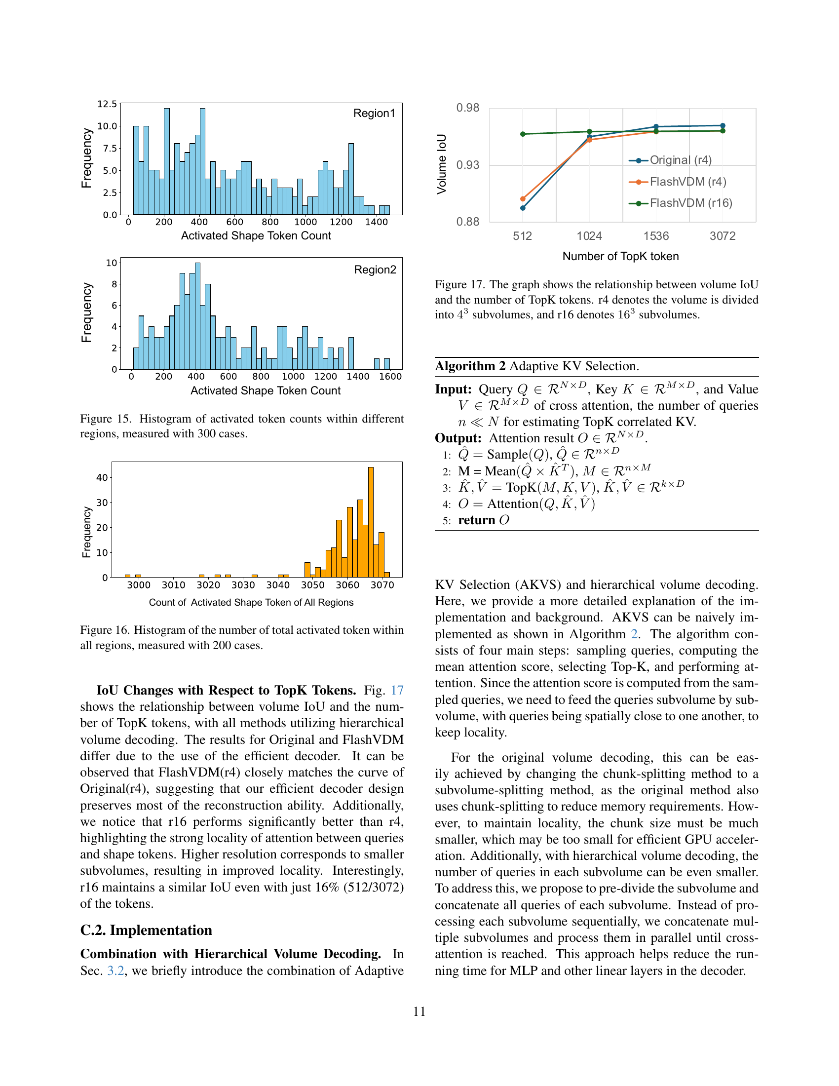
🔼 This figure presents histograms visualizing the distribution of activated token counts across different regions within a 3D volume. The data was collected from 300 distinct cases, each representing a unique shape generation scenario. Each histogram corresponds to a specific region within the volume. The x-axis represents the activated token counts, and the y-axis represents the frequency of occurrence for each token count. The histograms reveal the varying patterns of token activation across different regions. These patterns offer insights into the locality of attention mechanisms employed in the shape decoding process.
read the caption
Figure 15: Histogram of activated token counts within different regions, measured with 300 cases.

🔼 This histogram visualizes the distribution of the total count of activated tokens across 200 different cases in the Adaptive KV Selection method. The x-axis represents the total number of activated tokens observed in a single case. The y-axis indicates the frequency or number of cases exhibiting that specific total token count. This figure demonstrates the distribution of activated tokens, providing insights into the efficiency and potential for reduction within the Adaptive KV Selection mechanism. It helps support the claim that most regions don’t need many keys, and therefore the adaptive method can significantly reduce the computational load.
read the caption
Figure 16: Histogram of the number of total activated token within all regions, measured with 200 cases.

🔼 This figure illustrates the effect of the number of top-k tokens (key-value pairs selected from the original set) on volume Intersection over Union (IoU), a measure of 3D reconstruction accuracy. Two scenarios are compared: dividing the volume into 4^3=64 subvolumes (r4) and 16^3=4096 subvolumes (r16). The graph reveals the trade-off between computational efficiency (fewer tokens) and reconstruction accuracy. It demonstrates that using a smaller subset of tokens (lower TopK values) can significantly reduce computation but may slightly decrease IoU, depending on the level of volume subdivision (r4 vs r16).
read the caption
Figure 17: The graph shows the relationship between volume IoU and the number of TopK tokens. r4 denotes the volume is divided into 43superscript434^{3}4 start_POSTSUPERSCRIPT 3 end_POSTSUPERSCRIPT subvolumes, and r16 denotes 163superscript16316^{3}16 start_POSTSUPERSCRIPT 3 end_POSTSUPERSCRIPT subvolumes.

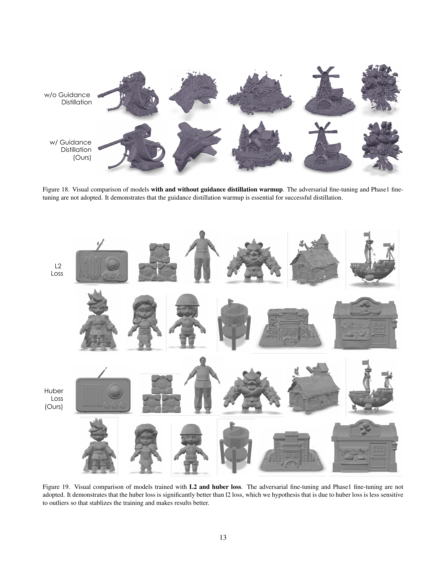
🔼 This figure compares the results of models trained with and without guidance distillation warmup. The experiment intentionally omits adversarial fine-tuning and Phase 1 fine-tuning to isolate the effect of the warmup phase. The comparison visually demonstrates that guidance distillation warmup is crucial for successful distillation in this specific context. Without the warmup, the generated 3D models are significantly less coherent and detailed.
read the caption
Figure 18: Visual comparison of models with and without guidance distillation warmup. The adversarial fine-tuning and Phase1 fine-tuning are not adopted. It demonstrates that the guidance distillation warmup is essential for successful distillation.

🔼 This figure compares 3D model generation results using L2 loss and Huber loss during training. Both sets of models were trained without adversarial fine-tuning or Phase 1 fine-tuning to isolate the effect of the loss function. The results demonstrate that the Huber loss produces significantly better quality 3D models. The authors hypothesize this is because Huber loss is less sensitive to outliers in the training data, leading to more stable training and improved model performance.
read the caption
Figure 19: Visual comparison of models trained with L2 and huber loss. The adversarial fine-tuning and Phase1 fine-tuning are not adopted. It demonstrates that the huber loss is significantly better than l2 loss, which we hypothesis that is due to huber loss is less sensitive to outliers so that stablizes the training and makes results better.

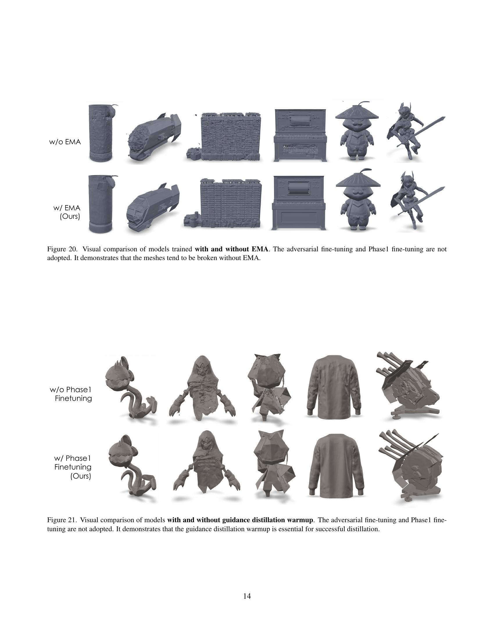
🔼 This figure presents a visual comparison of 3D models generated using two different training methods: one with Exponential Moving Average (EMA) and another without. The models are trained using the same parameters except for the EMA. The goal is to show that the use of EMA significantly improves the quality of the generated 3D meshes. The absence of EMA results in models producing fragmented, broken meshes, highlighting EMA’s crucial role in model stability and the generation of high-quality 3D structures.
read the caption
Figure 20: Visual comparison of models trained with and without EMA. The adversarial fine-tuning and Phase1 fine-tuning are not adopted. It demonstrates that the meshes tend to be broken without EMA.

🔼 This figure compares the results of training a diffusion model for 3D shape generation with and without a guidance distillation warmup phase. The experiment specifically omits adversarial fine-tuning and Phase 1 fine-tuning to isolate the effect of the warmup. The results demonstrate that including the guidance distillation warmup step is crucial for achieving successful distillation and effective model training. Without the warmup, the resulting model’s performance suffers significantly.
read the caption
Figure 21: Visual comparison of models with and without guidance distillation warmup. The adversarial fine-tuning and Phase1 fine-tuning are not adopted. It demonstrates that the guidance distillation warmup is essential for successful distillation.

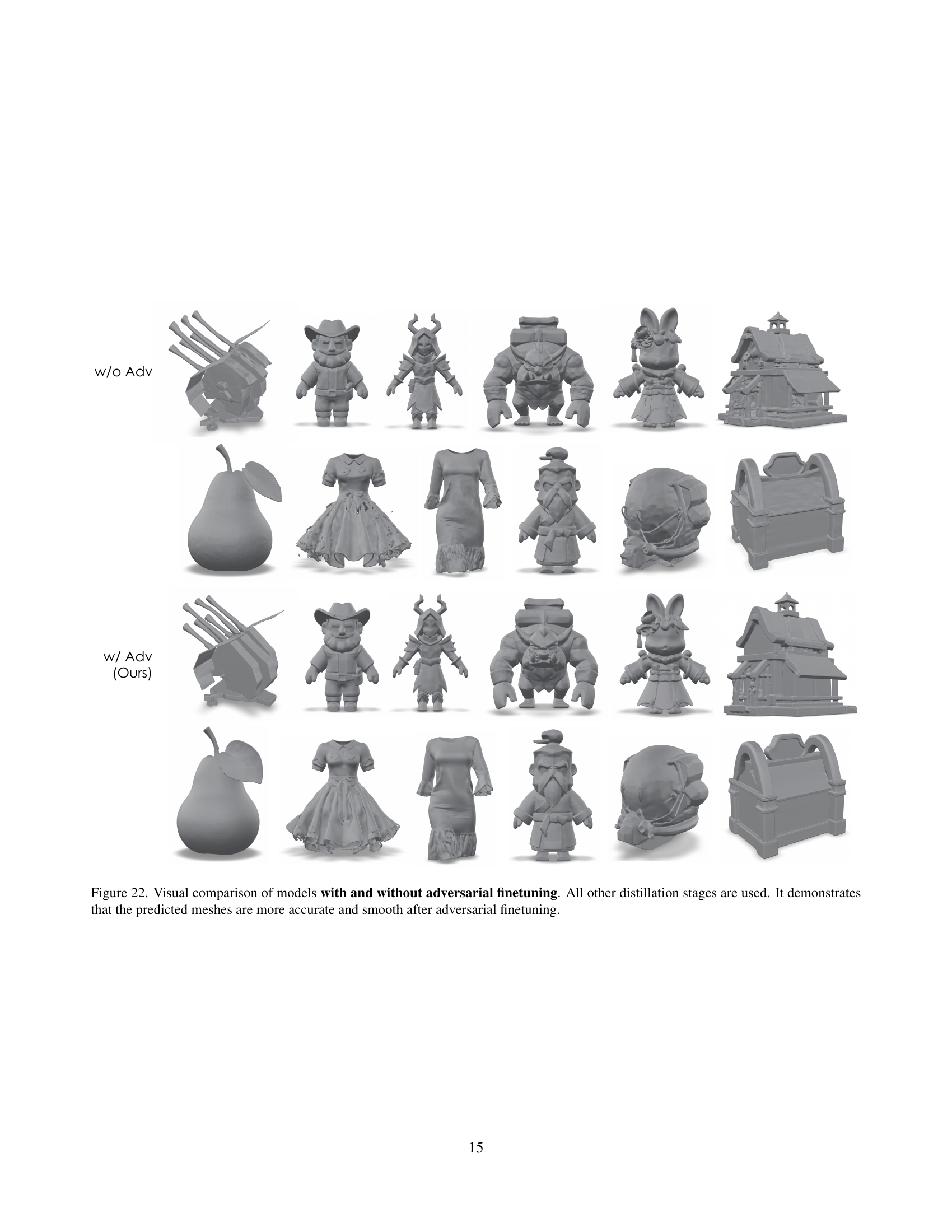
🔼 This figure compares 3D model outputs generated with and without adversarial fine-tuning during the training process. All other stages of the distillation process (progressive flow distillation) were identical in both cases. The results show that adding adversarial fine-tuning leads to more accurate and smoother 3D mesh surfaces in the generated models.
read the caption
Figure 22: Visual comparison of models with and without adversarial finetuning. All other distillation stages are used. It demonstrates that the predicted meshes are more accurate and smooth after adversarial finetuning.

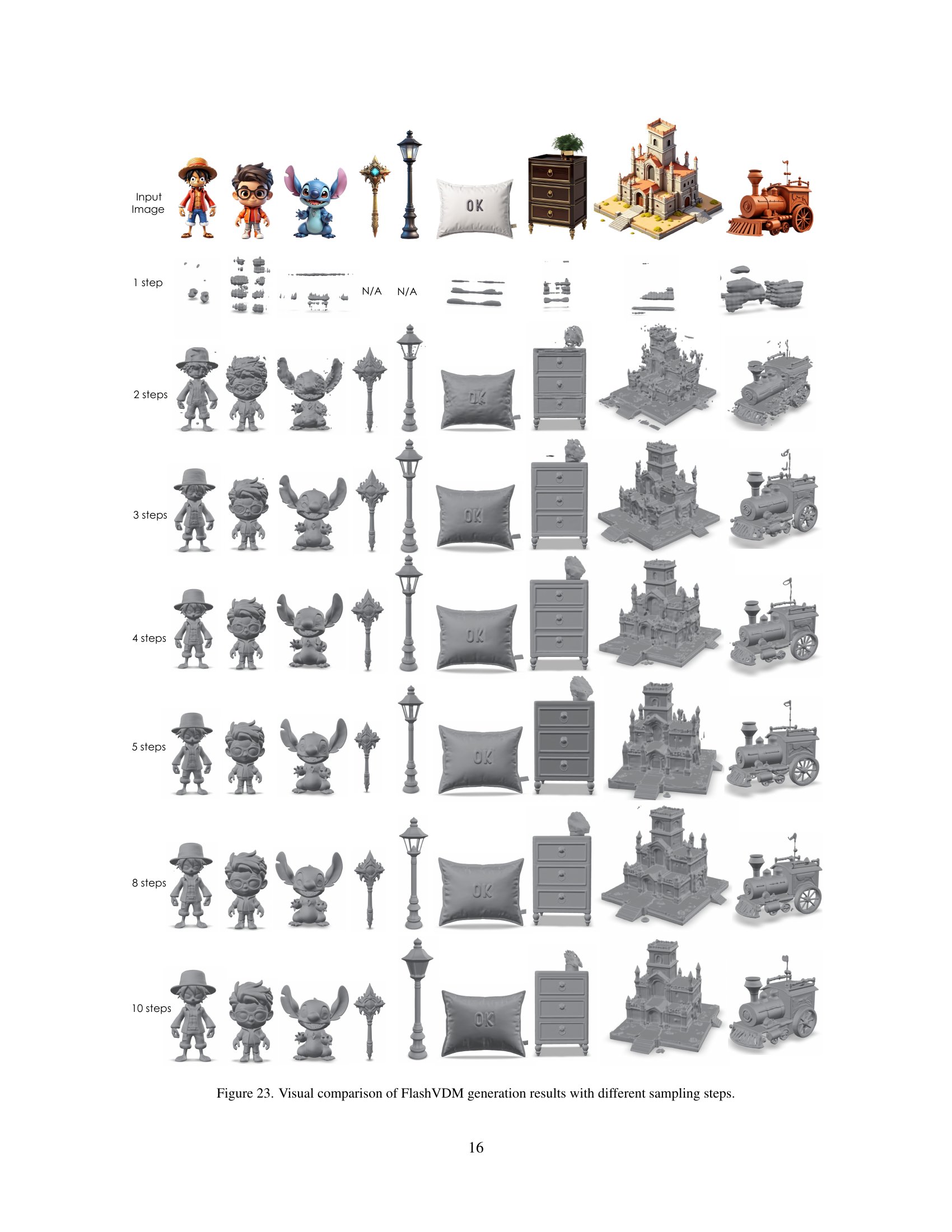
🔼 This figure shows a comparison of 3D model generation results from FlashVDM using different numbers of sampling steps (1, 2, 3, 4, 5, 8, and 10). Each row represents a different number of steps, and each column shows the same set of objects generated with that number of steps. It demonstrates how the quality of the generated models increases as the number of sampling steps increases.
read the caption
Figure 23: Visual comparison of FlashVDM generation results with different sampling steps.

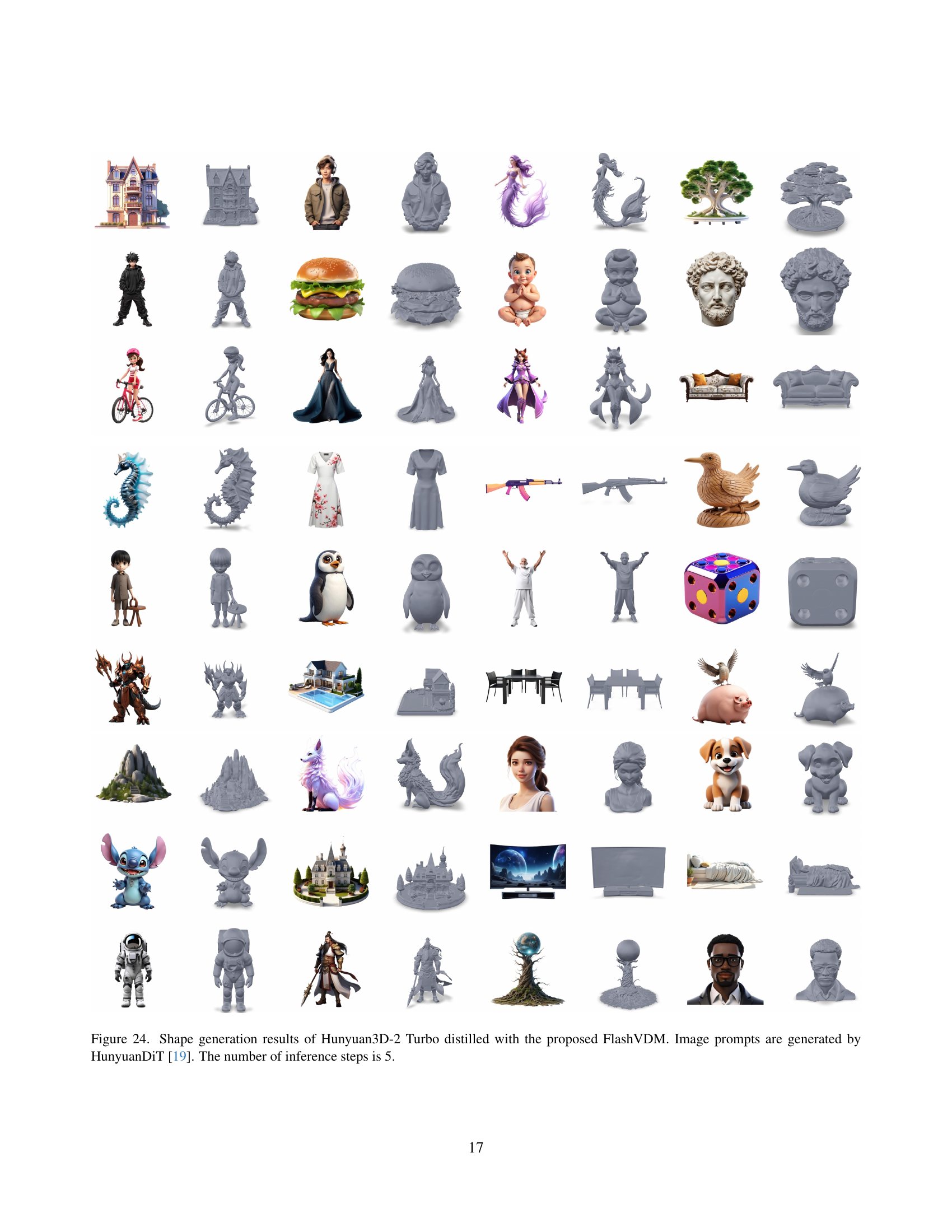
🔼 This figure showcases the results of shape generation using the Hunyuan3D-2 Turbo model, enhanced by the FlashVDM framework. A variety of 3D shapes are displayed, all generated from different image prompts produced by the HunyuanDiT model. The process involved only 5 inference steps, highlighting the speed and efficiency of the FlashVDM method. The figure demonstrates the high-quality, detailed 3D shapes generated despite the minimal number of steps, showcasing the effectiveness of FlashVDM in accelerating shape generation.
read the caption
Figure 24: Shape generation results of Hunyuan3D-2 Turbo distilled with the proposed FlashVDM. Image prompts are generated by HunyuanDiT [19]. The number of inference steps is 5.

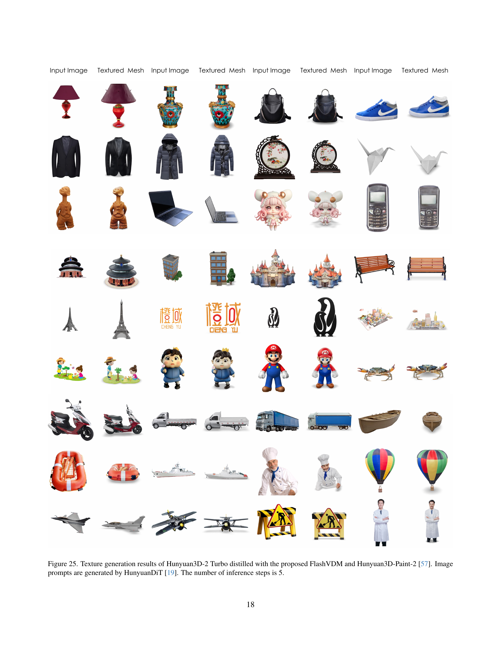
🔼 This figure showcases the results of applying the FlashVDM model to generate textures for 3D shapes. Specifically, it uses the Hunyuan3D-2 Turbo model (a pre-trained Vecset Diffusion Model), enhanced with FlashVDM for faster processing. The textures are generated using image prompts created by the HunyuanDiT model. The results demonstrate the effectiveness of FlashVDM in improving speed and quality by completing the texturing process within only 5 diffusion sampling steps. The figure presents multiple examples of image prompts alongside the generated textured 3D meshes, offering a visual comparison of input and output.
read the caption
Figure 25: Texture generation results of Hunyuan3D-2 Turbo distilled with the proposed FlashVDM and Hunyuan3D-Paint-2 [57]. Image prompts are generated by HunyuanDiT [19]. The number of inference steps is 5.
More on tables
| ULIP-I() | Uni3D-I() | Time(s) | |
| TripoSR [42] | 0.0642 | 0.1425 | 0.958 |
| SF3D [3] | 0.1156 | 0.2676 | 0.212 |
| SPAR3D [11] | 0.1149 | 0.2679 | 1.296 |
| Trellis [46] | 0.1267 | 0.3116 | 7.334 |
| Hunyuan3D-2 [59] | 0.1303 | 0.3151 | 34.85 |
| with FlashVDM | 0.1260 | 0.3095 | 1.041 |
🔼 This table presents a quantitative comparison of different shape generation methods, focusing on three key metrics: ULIP-I (a metric for evaluating the similarity between the generated mesh and input images), Uni3D-I (another metric measuring the similarity), and the generation time. The table allows for a direct comparison of the performance of various methods, including the proposed FlashVDM, in terms of both accuracy and speed.
read the caption
Table 2: Numerical comparisons of shape generation methods.
| V-IoU() | S-IoU() | Time(s) | |
| VAE Baseline | 96.11% | 93.27% | 22.33 |
| + Hierarchical Decoding | 96.11% | 93.27% | 2.322 |
| + Efficient Decoder | 96.08% | 93.13% | 0.731 |
| + Adaptive KV Selection | 95.55% | 93.10% | 0.491 |
🔼 This table presents a detailed breakdown of the performance improvements achieved by incrementally adding each component of the proposed ’lightning vecset decoder’. It shows the effects on Volume IoU (V-IoU), Surface IoU (S-IoU), and decoding time as each component (Hierarchical Volume Decoding, Efficient Decoder, and Adaptive KV Selection) is added to the baseline VAE decoder. This allows for a clear understanding of the individual contributions of each component to the overall speed and accuracy improvements.
read the caption
Table 3: Step-by-step ablation of our lightning vecset decoder.
Full paper#