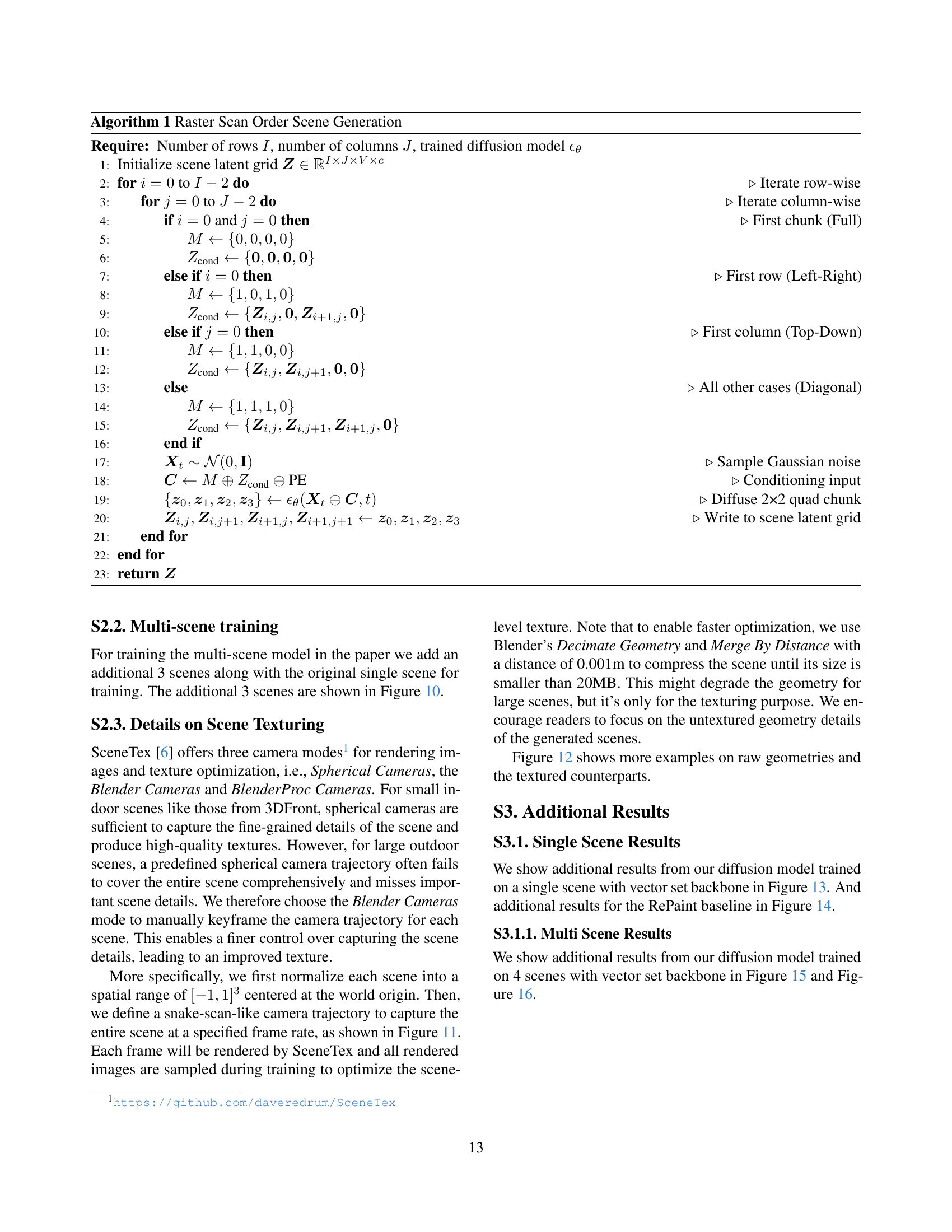
TL;DR#
Generating expansive outdoor scenes is crucial for VR, games, and CGI, but is traditionally labor-intensive. Unlike indoor scenes, outdoor environments present unique challenges like varying heights and rapid landscape creation. Existing methods are limited by low geometric quality and scene variation. Solutions for unbounded indoor scenes struggle with skyscrapers and high memory usage, as they rely on spatially structured latents like triplanes or dense feature grids. Scaling these methods for outdoor environments results in inefficiency and detail loss. Datasets lack high-quality geometry and height variation, hindering effective model training.
This paper explores generating large outdoor scenes with NuiScene, ranging from castles to high-rises, through an efficient approach that encodes scene chunks as uniform vector sets for improved compression. An outpainting model is trained to enhance coherence and speed up the generation. The team curates a small but high-quality dataset, enabling joint training on scenes of varying styles. The work facilitates blending of different environments, such as rural houses and city skyscrapers within the same scene.
Key Takeaways#
Why does it matter?#
This paper on the NuiScene dataset and methodology helps lower the barrier for outdoor scene generation. It enables researchers to explore AI-driven world-building for games, VR, and film more efficiently. The method improves scene creation speed and cohesion, opening doors for more complex virtual environments.
Visual Insights#

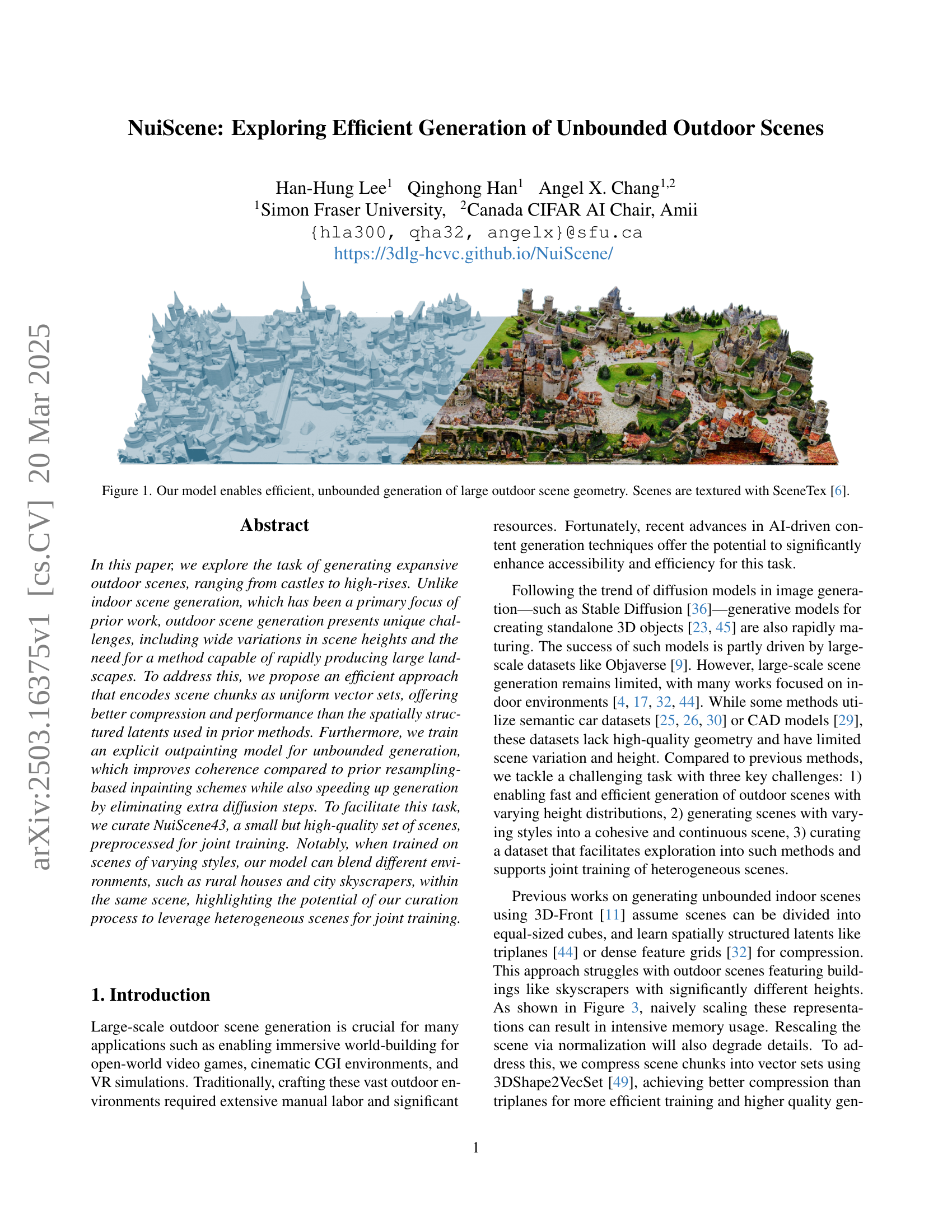
🔼 This figure showcases the capabilities of the model to generate expansive and coherent outdoor scenes efficiently. It displays multiple examples of large-scale outdoor environments, demonstrating the model’s ability to handle diverse scene geometries and details. The scenes presented include various elements, such as castles, high-rises, and natural landscapes, highlighting the model’s capacity for generating complex and diverse environments. Note that the scenes in the image have been textured using SceneTex.
read the caption
Figure 1: Our model enables efficient, unbounded generation of large outdoor scene geometry. Scenes are textured with SceneTex [6].
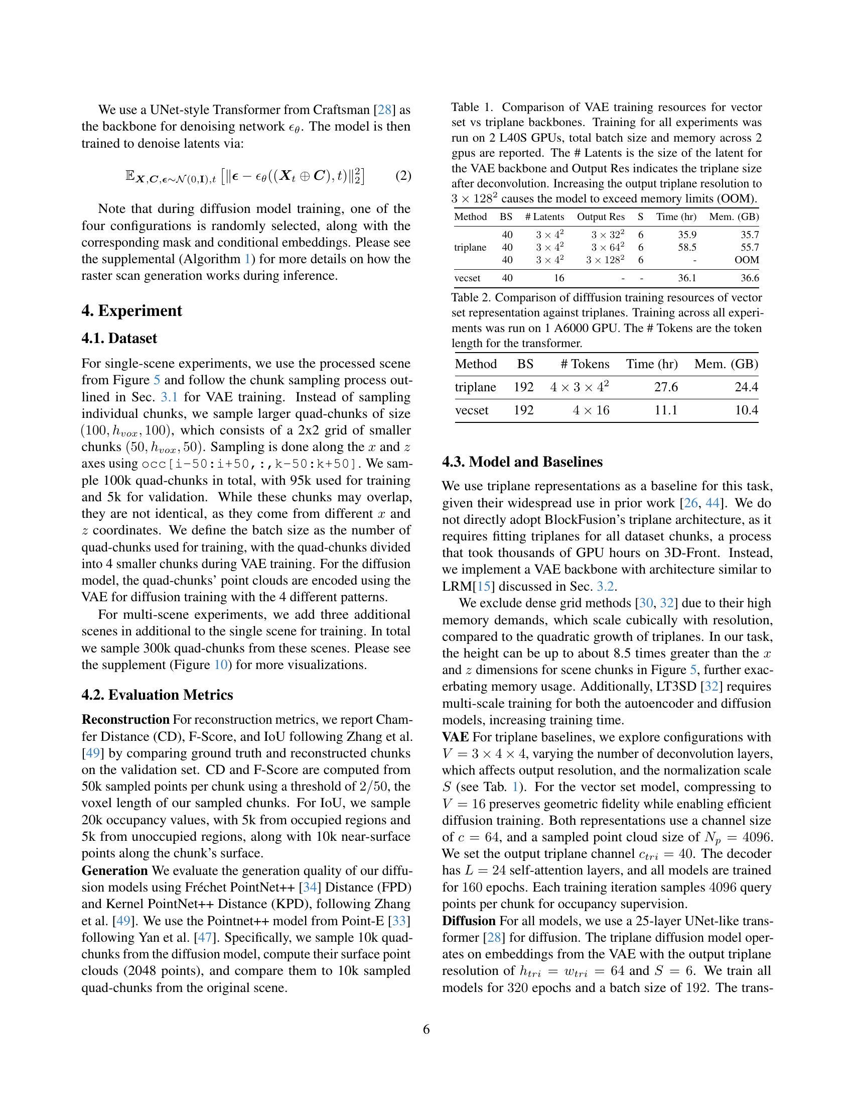
| Method | BS | # Latents | Output Res | S | Time (hr) | Mem. (GB) |
| triplane | 40 | 6 | 35.9 | 35.7 | ||
| 40 | 6 | 58.5 | 55.7 | |||
| 40 | 6 | - | OOM | |||
| vecset | 40 | 16 | - | - | 36.1 | 36.6 |
🔼 This table presents a quantitative comparison of 3D scene reconstruction results using different Variational Autoencoders (VAEs) as backbones. It evaluates the performance of reconstruction using two different height measurements: 1. ĥ (h-hat): Reconstruction using the predicted height of the scene chunk. 2. ~h (h-tilde): Reconstruction using the ground truth height of the scene chunk. The table compares the performance across various VAE architectures using metrics such as Intersection over Union (IoU), Chamfer Distance (CD), and F-Score. These metrics provide insights into the accuracy and completeness of the reconstructed scenes, highlighting the impact of the VAE choice on the reconstruction’s fidelity and efficiency.
read the caption
Table 3: Quantitative comparison of reconstruction across different VAE backbones. Here h^^ℎ\hat{h}over^ start_ARG italic_h end_ARG indicates that the predicted height was used for the occupancy prediction and h~~ℎ\tilde{h}over~ start_ARG italic_h end_ARG the ground truth height.
In-depth insights#
Unbounded Gen#
The research delves into the complexities of unbounded scene generation, differentiating itself from prior work often confined to indoor environments. A significant challenge lies in handling the vast height variations typical of outdoor scenes, like skyscrapers dwarfing smaller structures. Existing methods that rely on spatially structured latents, such as triplanes or dense feature grids, struggle with scalability and memory efficiency when applied to scenes with such diverse heights. Naive scaling leads to either memory overload or detail loss. To overcome these limitations, the paper introduces a more efficient approach using vector sets for compressing scene chunks, promising better performance and compression compared to spatially structured latents. The introduction of an explicit outpainting model further addresses the need for coherent, unbounded generation by learning to predict new chunks conditioned on existing ones. This avoids extra diffusion steps associated with resampling-based inpainting, enabling faster and more efficient scene creation.
Vector vs Triplane#
The vector vs. triplane analysis centers on comparing different latent space representations for scene generation. Vector sets offer a compact, uniform representation, especially beneficial for scenes with varying heights, as seen in outdoor environments. They avoid the memory issues and detail loss that occur when naively scaling triplanes, a spatially structured latent space. Triplanes might struggle with tall structures due to coordinate clamping, where as vector representation better compresses and can handle scaling with flexible querying due to their cross-attention mechanism. Also vector representation is less computationally intensive in terms of memory requirements.
Explicit Outpaint#
The concept of ‘Explicit Outpainting’ represents a strategic shift in generative modeling, particularly for unbounded scenes. Instead of relying on iterative, resampling-based inpainting techniques like RePaint, this approach advocates for directly training a diffusion model to generate content outside the existing boundaries. This tackles limitations of methods requiring extra diffusion steps, thus improving the speed. By conditioning the generation on whole, previously generated chunks, context is preserved effectively, potentially enhancing coherency. ‘Explicit’ training may allow greater control over style and content in the new areas, also reducing error accumulation from repeated resampling. By streamlining generation, explicit outpainting offers an efficient way to create large, continuous environments, while maintaining quality.
Hetero. Training#
Heterogeneous training, a concept not explicitly detailed in the provided text, could involve training a model using diverse data sources or architectures. This might entail leveraging datasets with varying levels of quality or annotation, necessitating strategies to mitigate bias and ensure robust performance. Alternatively, it could refer to employing different model architectures within a single training pipeline, such as combining convolutional and transformer networks to capture complementary features. The potential benefits include improved generalization, adaptability to diverse input modalities, and enhanced robustness against adversarial attacks. However, challenges may arise in terms of data alignment, model synchronization, and computational complexity. Careful consideration must be given to weighting the contributions of different data sources or architectures, as well as developing effective strategies for knowledge transfer and fusion. Data curation, preprocessing techniques, and suitable network architectures are also really important.
NuiScene43 Limit#
Considering a hypothetical section titled “NuiScene43 Limit,” it likely discusses the constraints and boundaries of the NuiScene43 dataset. This could encompass several aspects. One major limitation probably revolves around the dataset size; with only 43 scenes, the diversity of environments might be restricted, potentially leading to overfitting or a lack of generalization to completely novel scene types. Another constraint could be the resolution and detail of the 3D meshes within NuiScene43. Pre-processing steps, such as ground fixing, although beneficial for training, can simplify the original data. The dataset might also face limitations related to annotation quality and scope. Finally, the limited dataset size could impact the controllability of the generative model, making it difficult to condition the generation on specific attributes or styles effectively.
More visual insights#
More on figures

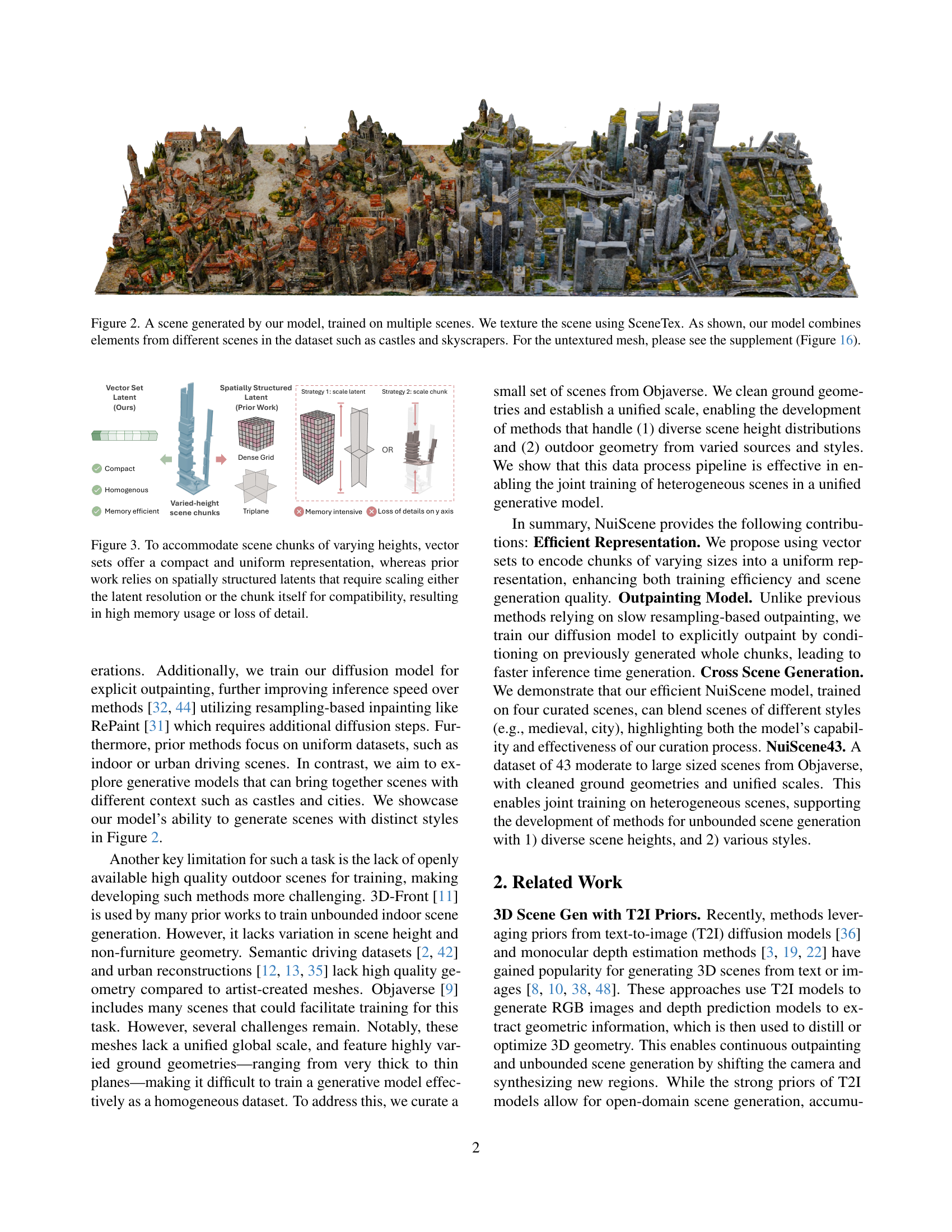
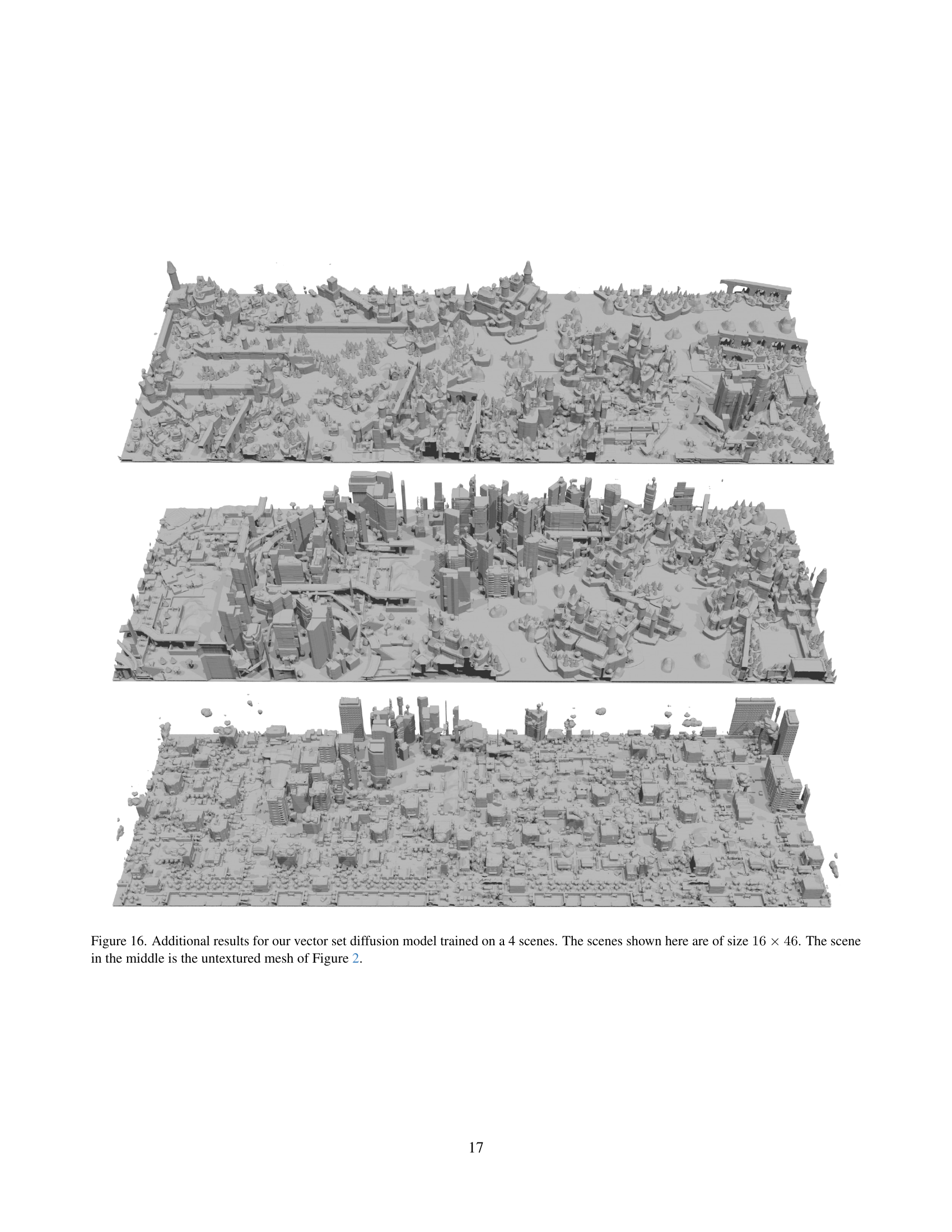
🔼 This figure showcases a scene generated by the model which is trained on multiple scenes from the NuiScene43 dataset. The scene demonstrates the model’s ability to combine elements from diverse architectural styles, including castles and skyscrapers, into a cohesive whole. The scene is textured using SceneTex. The supplemental material (Figure 16) provides a view of the untextured mesh for further analysis.
read the caption
Figure 2: A scene generated by our model, trained on multiple scenes. We texture the scene using SceneTex. As shown, our model combines elements from different scenes in the dataset such as castles and skyscrapers. For the untextured mesh, please see the supplement (Figure 16).

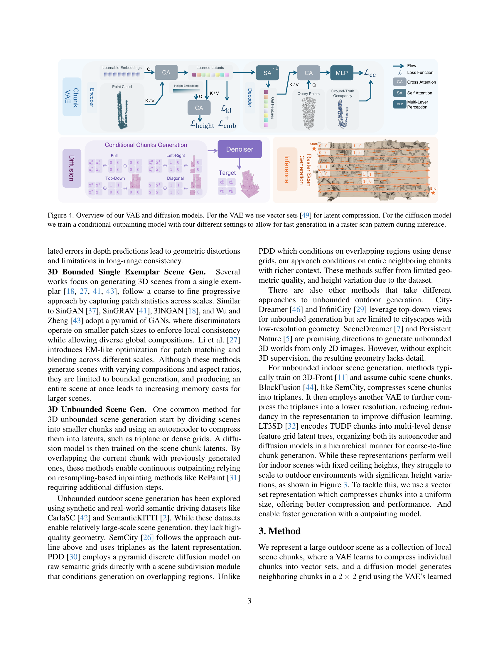
🔼 This figure compares different latent representations used in generating 3D scenes with varying heights. Spatially structured latents, such as triplanes, struggle with scenes containing varied heights. Scaling either the latent resolution or the chunk size to accommodate different heights leads to memory issues or loss of detail. In contrast, vector sets provide a compact and uniform representation that efficiently handles scenes with varying heights, thus avoiding memory problems and detail loss.
read the caption
Figure 3: To accommodate scene chunks of varying heights, vector sets offer a compact and uniform representation, whereas prior work relies on spatially structured latents that require scaling either the latent resolution or the chunk itself for compatibility, resulting in high memory usage or loss of detail.

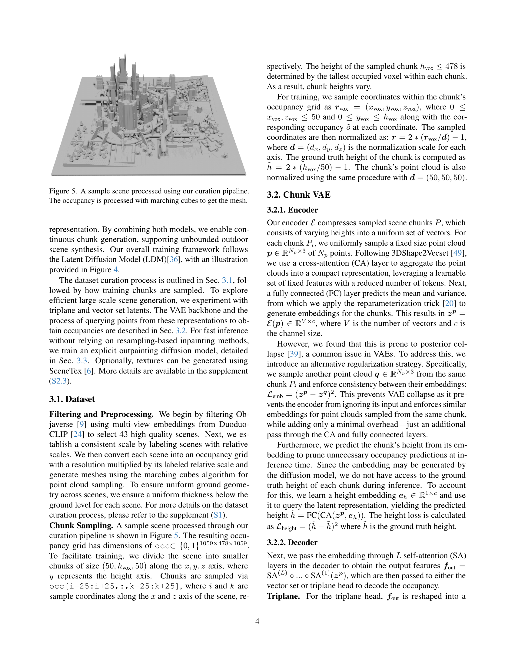
🔼 This figure illustrates the architecture of the VAE (Variational Autoencoder) and diffusion models used in the paper. The VAE uses vector sets for efficient compression of the latent space, representing scene chunks as uniform vector sets instead of spatially structured latents which improves memory efficiency and performance. The diffusion model is designed for outpainting, allowing the model to efficiently generate unbounded scenes. It incorporates four different conditioning settings during training to facilitate fast generation in a raster-scan pattern during inference. This ensures that the model can seamlessly generate new chunks of the scene by taking into account the previously generated parts. The diagram details the data flow for both the encoder and decoder stages in the VAE, as well as the input and output elements of the diffusion model, highlighting the conditional outpainting process.
read the caption
Figure 4: Overview of our VAE and diffusion models. For the VAE we use vector sets [49] for latent compression. For the diffusion model we train a conditional outpainting model with four different settings to allow for fast generation in a raster scan pattern during inference.

🔼 This figure shows a sample scene after undergoing the data curation pipeline described in the paper. The pipeline involves several steps, including filtering Objaverse to select high-quality scenes, establishing a consistent scale across scenes, and converting the mesh to an occupancy grid. This occupancy grid is then used as input for the marching cubes algorithm, which generates a 3D mesh. The resulting mesh is a more refined representation of the scene suitable for training the model.
read the caption
Figure 5: A sample scene processed using our curation pipeline. The occupancy is processed with marching cubes to get the mesh.

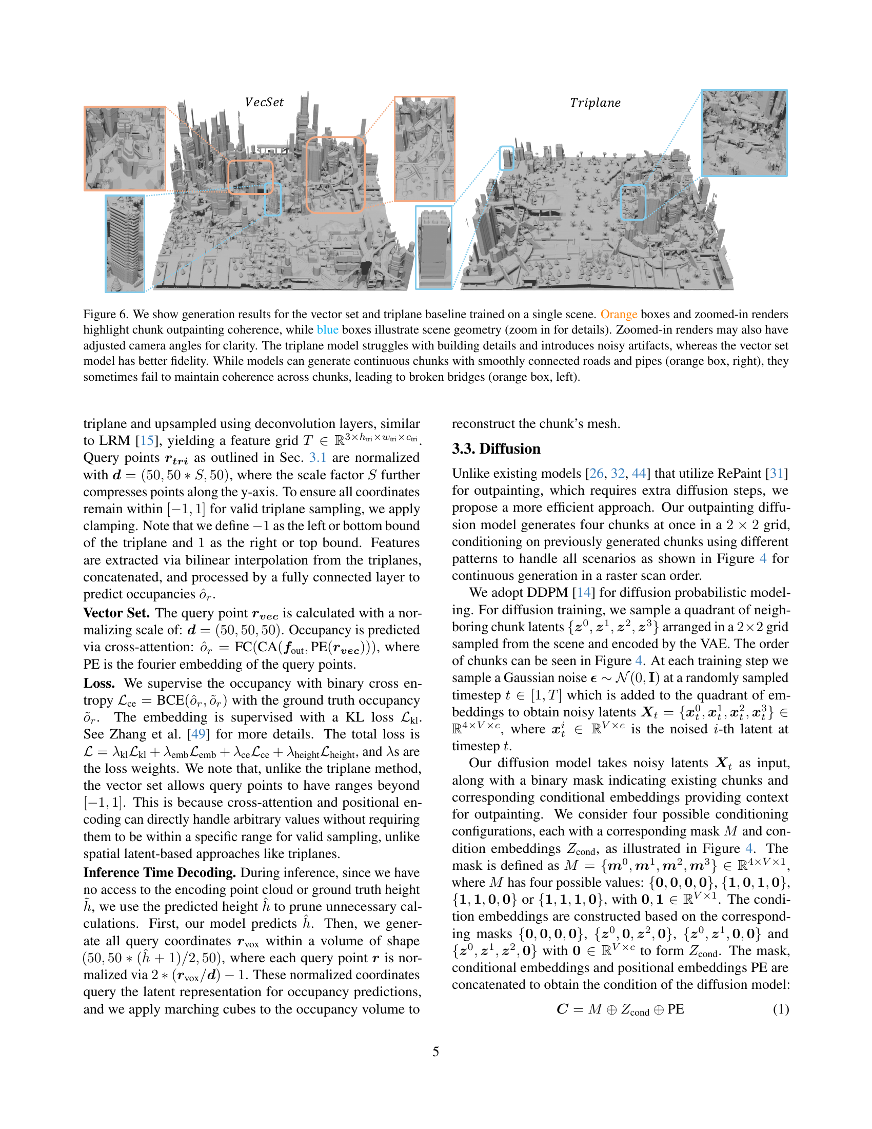
🔼 This figure compares the performance of vector set and triplane methods for generating unbounded outdoor scenes. The vector set method demonstrates superior performance in terms of detail and coherence, while the triplane method struggles with details and introduces artifacts. The images highlight differences in how smoothly the models generate contiguous sections of the scene, particularly noticeable in the examples of road and bridge construction where the triplane model shows more errors. This is shown through both full-scene renders and zoomed-in sections for detailed analysis.
read the caption
Figure 6: We show generation results for the vector set and triplane baseline trained on a single scene. Orange boxes and zoomed-in renders highlight chunk outpainting coherence, while blue boxes illustrate scene geometry (zoom in for details). Zoomed-in renders may also have adjusted camera angles for clarity. The triplane model struggles with building details and introduces noisy artifacts, whereas the vector set model has better fidelity. While models can generate continuous chunks with smoothly connected roads and pipes (orange box, right), they sometimes fail to maintain coherence across chunks, leading to broken bridges (orange box, left).

🔼 This table compares the computational resources required for training a Variational Autoencoder (VAE) with two different latent representations: vector sets and triplanes. The experiment used two NVIDIA L40S GPUs. The table shows the batch size, the size of the latent vector (#Latents), the output resolution of the triplane after deconvolution (Output Res), training time, and GPU memory usage. It highlights that increasing the triplane resolution significantly increases memory consumption, resulting in an out-of-memory (OOM) error.
read the caption
Table 1: Comparison of VAE training resources for vector set vs triplane backbones. Training for all experiments was run on 2 L40S GPUs, total batch size and memory across 2 gpus are reported. The # Latents is the size of the latent for the VAE backbone and Output Res indicates the triplane size after deconvolution. Increasing the output triplane resolution to 3×12823superscript12823\times 128^{2}3 × 128 start_POSTSUPERSCRIPT 2 end_POSTSUPERSCRIPT causes the model to exceed memory limits (OOM).
🔼 This table compares the computational resources required for training diffusion models using two different latent representations: vector sets and triplanes. The training was performed on a single NVIDIA A6000 GPU. The table shows the batch size used, the number of tokens in the transformer (related to model complexity), the total training time in hours, and the GPU memory (VRAM) used in gigabytes (GB). This allows for a comparison of the efficiency of each representation in terms of training time and memory usage.
read the caption
Table 2: Comparison of difffusion training resources of vector set representation against triplanes. Training across all experiments was run on 1 A6000 GPU. The # Tokens are the token length for the transformer.

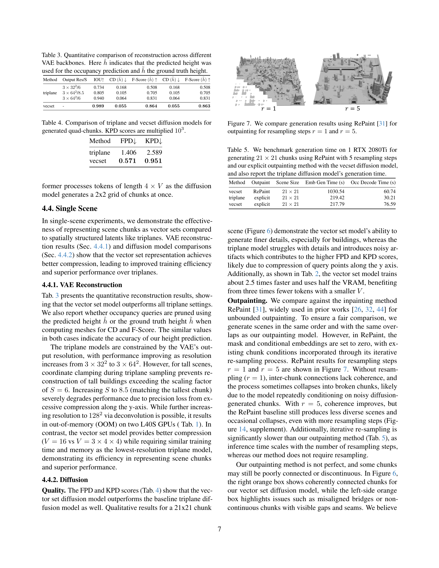
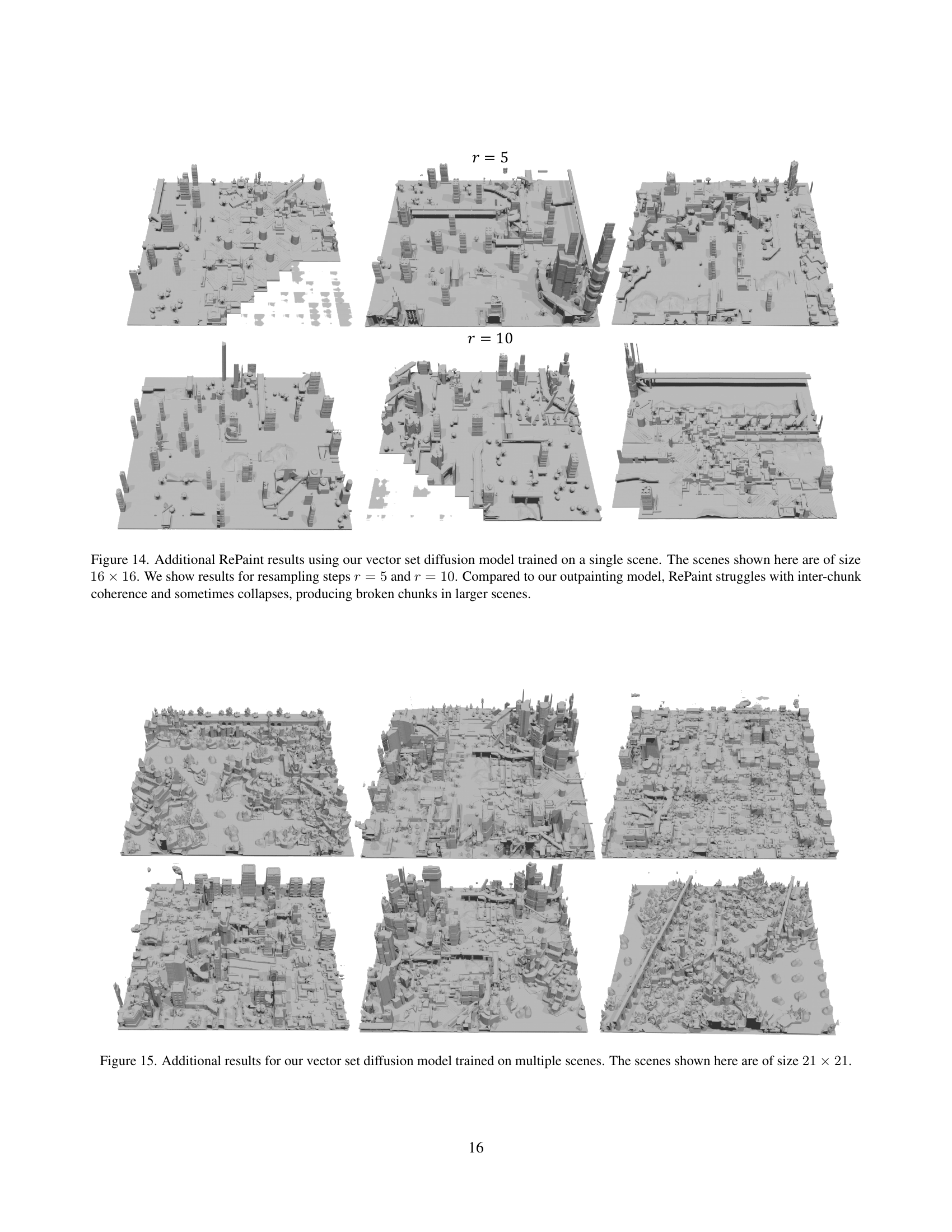
🔼 This figure compares the results of using RePaint, a resampling-based inpainting method, with different numbers of resampling steps (r=1 and r=5) for generating unbounded scenes. It visually demonstrates the impact of the number of resampling steps on the coherence and quality of the generated scene. More resampling steps generally lead to better coherence but at the cost of increased computational time.
read the caption
Figure 7: We compare generation results using RePaint [31] for outpainting for resampling steps r=1𝑟1r=1italic_r = 1 and r=5𝑟5r=5italic_r = 5.

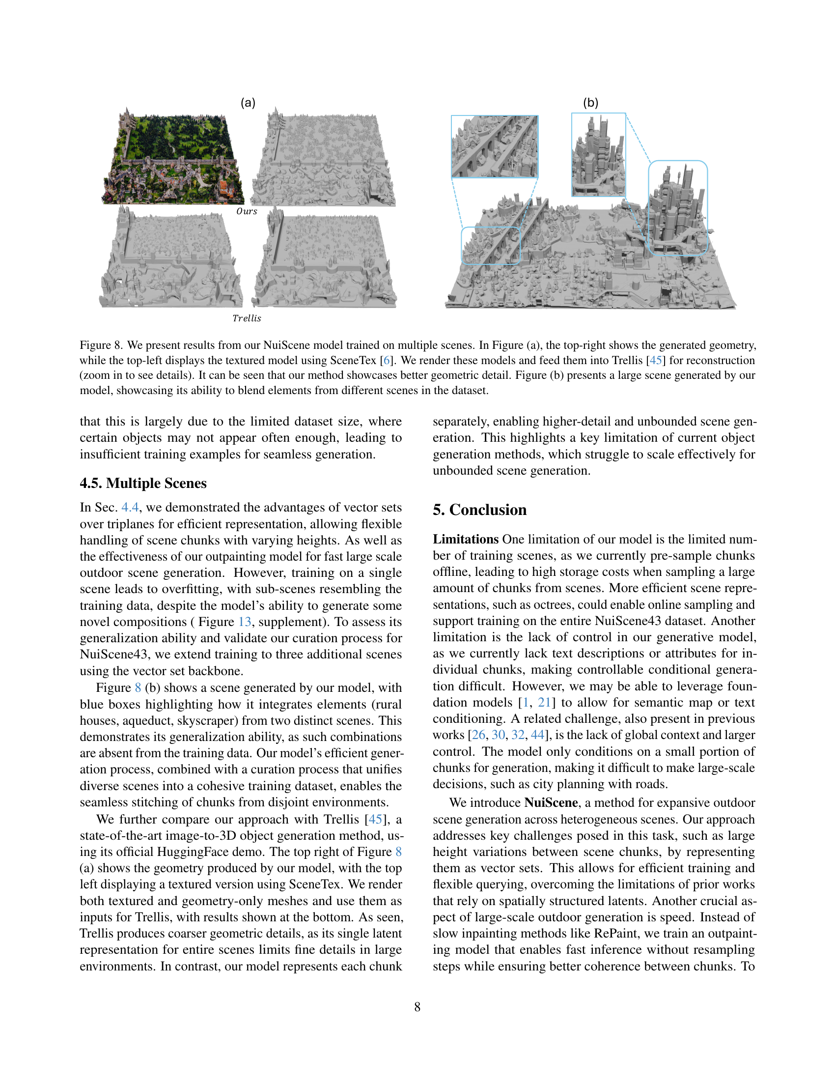
🔼 Figure 8 demonstrates the NuiScene model’s ability to generate large-scale outdoor scenes by blending elements from multiple source scenes. Part (a) compares the model’s output (top-right: raw geometry; top-left: textured using SceneTex) to the results of feeding the model’s output into a separate 3D reconstruction model, Trellis [45]. This comparison highlights the superior geometric detail preserved by the NuiScene model. Part (b) showcases a complete scene generated by NuiScene, demonstrating its ability to seamlessly integrate elements from diverse input scenes, creating a cohesive and complex environment.
read the caption
Figure 8: We present results from our NuiScene model trained on multiple scenes. In Figure (a), the top-right shows the generated geometry, while the top-left displays the textured model using SceneTex [6]. We render these models and feed them into Trellis [45] for reconstruction (zoom in to see details). It can be seen that our method showcases better geometric detail. Figure (b) presents a large scene generated by our model, showcasing its ability to blend elements from different scenes in the dataset.

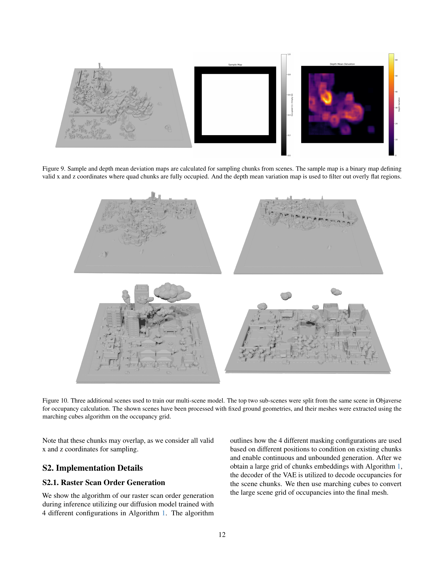
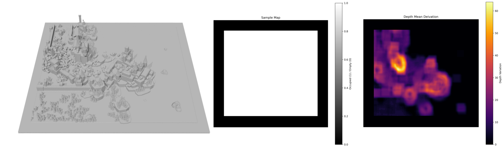
🔼 Figure 9 visualizes the process of selecting training data from scenes. Two maps are generated for each scene: a sample map and a depth mean deviation map. The sample map is a binary representation, where ‘1’ indicates fully occupied quad-chunk areas suitable for training data and ‘0’ shows empty areas. This ensures that only meaningful chunks are selected, improving the quality and efficiency of training. The depth mean deviation map provides a measure of depth variation within each chunk. This map is used as a filter, excluding overly flat regions from training data, further increasing training data quality and mitigating potential bias towards less diverse data.
read the caption
Figure 9: Sample and depth mean deviation maps are calculated for sampling chunks from scenes. The sample map is a binary map defining valid x and z coordinates where quad chunks are fully occupied. And the depth mean variation map is used to filter out overly flat regions.

🔼 Figure 10 shows three additional scenes used to train the multi-scene model. The top two scenes are actually sub-parts from the same scene in the Objaverse dataset. These three scenes were preprocessed to have consistent ground geometry before the meshes were extracted using the marching cubes algorithm from the occupancy grids.
read the caption
Figure 10: Three additional scenes used to train our multi-scene model. The top two sub-scenes were split from the same scene in Objaverse for occupancy calculation. The shown scenes have been processed with fixed ground geometries, and their meshes were extracted using the marching cubes algorithm on the occupancy grid.

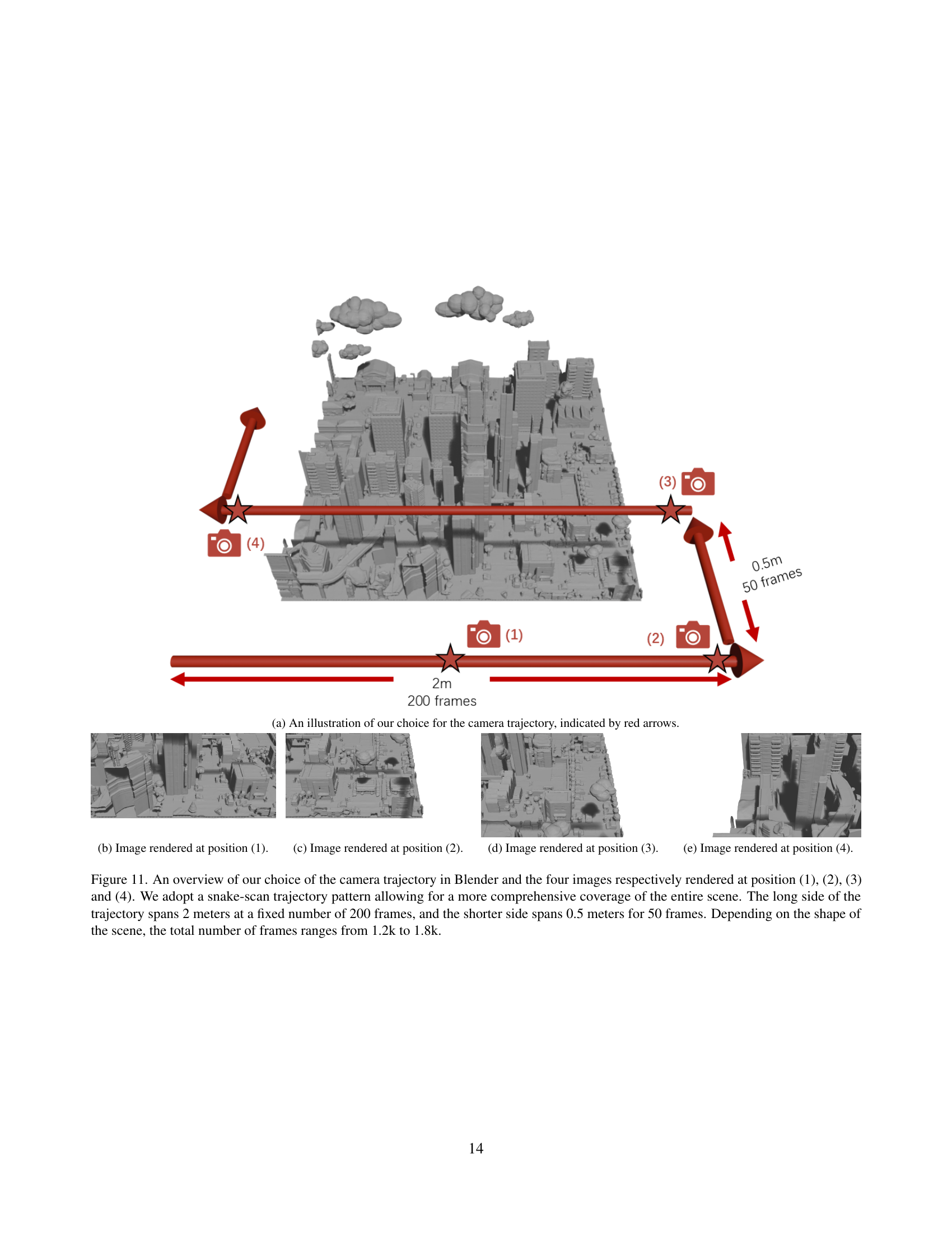
🔼 This figure illustrates the camera trajectory used for capturing images to generate textures for the scenes. The red arrows show the path of the camera, which is designed as a snake-scan pattern to ensure comprehensive coverage of the scene’s details. The long side of the trajectory covers 2 meters and consists of 200 frames, while the shorter side covers 0.5 meters and consists of 50 frames. The total number of frames depends on the scene’s shape and size, ranging from approximately 1200 to 1800 frames.
read the caption
(a) An illustration of our choice for the camera trajectory, indicated by red arrows.

🔼 This image shows a rendering of a scene from a specific camera position (position 1) as part of a camera trajectory used for capturing images to texture a large outdoor scene. The camera’s trajectory is designed for comprehensive coverage of the scene’s details and consists of multiple camera positions and viewpoints, ensuring that different parts of the scene are captured effectively. The rendered image provides a snapshot of the textured scene from one of the key viewpoints along this trajectory.
read the caption
(b) Image rendered at position (1).

🔼 This image is one of a series of images showing different viewpoints of a scene being rendered for texturing. The scene is an outdoor urban environment. The image shows a perspective view of the scene from a moderately high angle. The image is used to illustrate the sampling technique used for collecting data for training an AI model that creates similar scenes. This particular image shows a portion of a city with buildings and roads visible.
read the caption
(c) Image rendered at position (2).

🔼 This image shows one of the four viewpoints used in the creation of the camera trajectory for texturing the scene with SceneTex. The camera is positioned to capture a particular section of the large-scale outdoor scene. The full trajectory consists of multiple such viewpoints, each captured as a frame to ensure comprehensive coverage for accurate and high-quality texture synthesis. The placement of the viewpoints is designed to follow a snake-scan like pattern, creating a systematic coverage of the entire scene.
read the caption
(d) Image rendered at position (3).
🔼 This image shows a rendering of a scene from a specific camera position in a simulated environment. The camera is positioned as part of a snake-scan trajectory used for generating textures of large outdoor environments. This particular viewpoint is one of four shown to illustrate the comprehensive coverage of the scene provided by the chosen camera path. The whole sequence of images taken along the path is used to generate textures for the outdoor scenes.
read the caption
(e) Image rendered at position (4).

🔼 This figure illustrates the camera trajectory used for capturing high-quality textures of outdoor scenes using SceneTex. A snake-scan pattern is employed, ensuring comprehensive scene coverage. The longer side of the trajectory covers 2 meters across 200 frames, while the shorter side covers 0.5 meters in 50 frames. The total number of frames varies between 1200 and 1800 depending on scene dimensions. The figure displays four example images rendered from different viewpoints along this trajectory.
read the caption
Figure 11: An overview of our choice of the camera trajectory in Blender and the four images respectively rendered at position (1), (2), (3) and (4). We adopt a snake-scan trajectory pattern allowing for a more comprehensive coverage of the entire scene. The long side of the trajectory spans 2 meters at a fixed number of 200 frames, and the shorter side spans 0.5 meters for 50 frames. Depending on the shape of the scene, the total number of frames ranges from 1.2k to 1.8k.

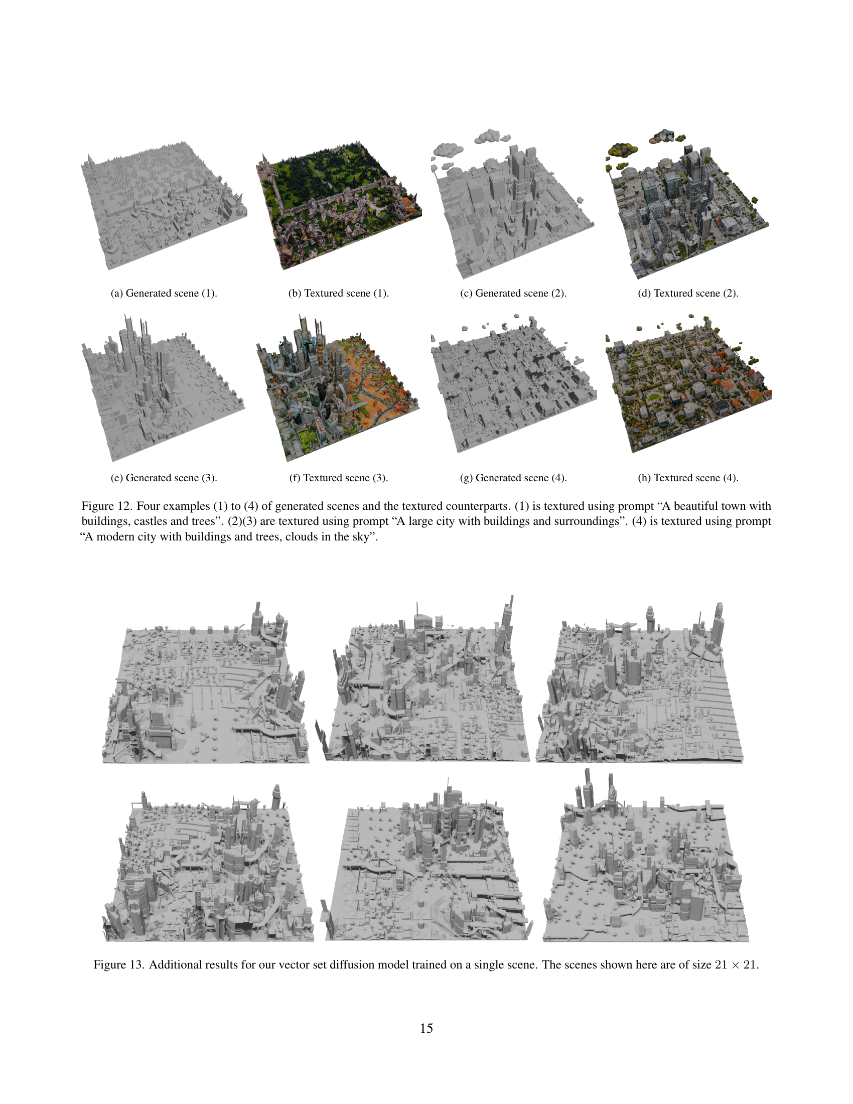
🔼 This figure shows a generated scene from the NuiScene model. The image showcases the model’s ability to generate realistic outdoor environments, demonstrating the quality of the geometry produced by the model. The generated scene includes a variety of elements, suggesting that the model has learned to combine different architectural styles and landscape features from its training data.
read the caption
(a) Generated scene (1).

🔼 This figure shows a textured 3D rendering of an outdoor scene generated by the model. The scene depicts a variety of elements, such as a castle-like structure, and appears to be set in a rural or medieval-style environment. The texture applied adds a high level of visual detail to the scene, making it look realistic and immersive.
read the caption
(b) Textured scene (1).

🔼 This figure shows a 21x21 chunk generated by the vector set diffusion model trained on a single scene. The image showcases the model’s ability to generate outdoor scenes with a variety of building styles and features, demonstrating its capacity for high-quality scene generation. Note that while the caption only says ‘(c) Generated Scene (2)’, this image is part of a larger figure illustrating multiple generated scenes.
read the caption
(c) Generated scene (2).

🔼 This figure shows a textured 3D rendering of a generated scene from the NuiScene model. The scene depicts a cityscape with various building types and surrounding environments. The texture is applied to the 3D model to create a more realistic and visually appealing representation of the generated scene.
read the caption
(d) Textured scene (2).

🔼 This figure showcases a 3D scene generated by the NuiScene model. The scene demonstrates the model’s ability to generate realistic outdoor environments, including a variety of building styles and landscaping features. The image is part of a series presented to illustrate the model’s capabilities in generating large-scale, coherent scenes from a dataset of diverse outdoor environments.
read the caption
(e) Generated scene (3).

🔼 This image displays a textured 3D rendering of an outdoor scene, generated by the model. The scene shows a variety of architectural styles and landscaping, showcasing the model’s ability to blend various elements seamlessly. This is one example in the supplementary material demonstrating the model’s ability to generate visually appealing and realistic scenes.
read the caption
(f) Textured scene (3).

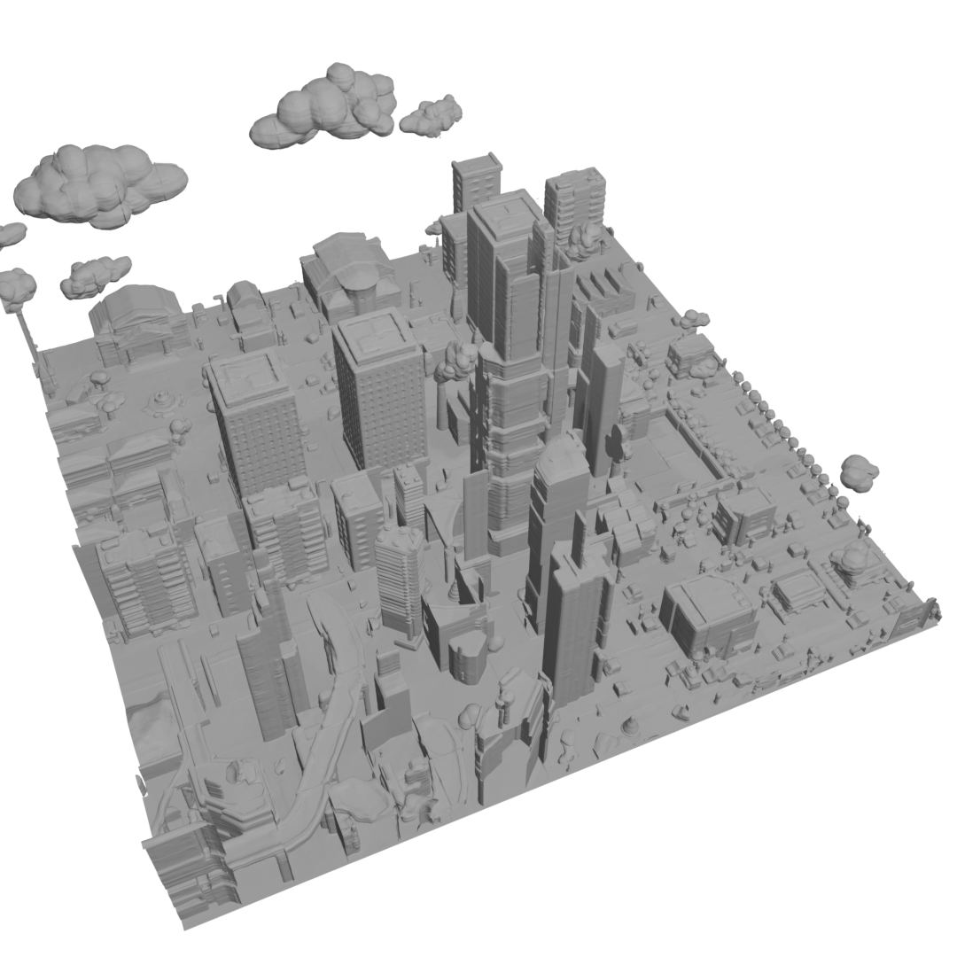
🔼 This figure shows a generated scene from the NuiScene model. The scene depicts a modern city with buildings and trees, and features clouds in the sky. The image is part of a series demonstrating the model’s ability to generate diverse and high-quality outdoor scenes.
read the caption
(g) Generated scene (4).

🔼 This image shows a textured 3D scene generated by the model, specifically scene number 4. The scene features a modern city with buildings and trees, and clouds in the sky. This texture was applied using SceneTex, highlighting the model’s ability to generate realistic and detailed outdoor environments.
read the caption
(h) Textured scene (4).
More on tables
| Method | BS | # Tokens | Time (hr) | Mem. (GB) |
| triplane | 192 | 27.6 | 24.4 | |
| vecset | 192 | 11.1 | 10.4 |
🔼 This table presents a quantitative comparison of the performance of two different latent space representations (triplane and vecset) within a diffusion model for generating 3D scene chunks. It shows the Fréchet PointNet++ Distance (FPD) and Kernel PointNet++ Distance (KPD) scores achieved by each method. Lower scores indicate better generation quality, representing a closer match between the generated and ground truth chunks. The KPD scores are multiplied by 1000 for easier interpretation.
read the caption
Table 4: Comparison of triplane and vecset diffusion models for generated quad-chunks. KPD scores are multiplied 103superscript10310^{3}10 start_POSTSUPERSCRIPT 3 end_POSTSUPERSCRIPT.
| Method | Output Res/S | IOU | CD | F-Score | CD | F-Score |
| triplane | / | 0.734 | 0.168 | 0.508 | 0.168 | 0.508 |
| / | 0.805 | 0.105 | 0.705 | 0.105 | 0.705 | |
| / | 0.940 | 0.064 | 0.831 | 0.064 | 0.831 | |
| vecset | - |
🔼 This table compares the generation time of 21x21 chunks using three different methods on an RTX 2080Ti GPU. The methods compared are: RePaint (an iterative inpainting method) with 5 resampling steps, the proposed explicit outpainting method using vector sets, and a baseline method using triplanes. The table shows the generation time broken down into two parts: the time taken to generate the chunk embeddings and the time taken to decode the occupancy and generate the mesh. This allows for a detailed performance comparison of the different approaches, highlighting the efficiency gains of the proposed method.
read the caption
Table 5: We benchmark generation time on 1 RTX 2080Ti for generating 21×21212121\times 2121 × 21 chunks using RePaint with 5 resampling steps and our explicit outpainting method with the vecset diffusion model, and also report the triplane diffusion model’s generation time.
| Method | FPD | KPD |
| triplane | 1.406 | 2.589 |
| vecset |
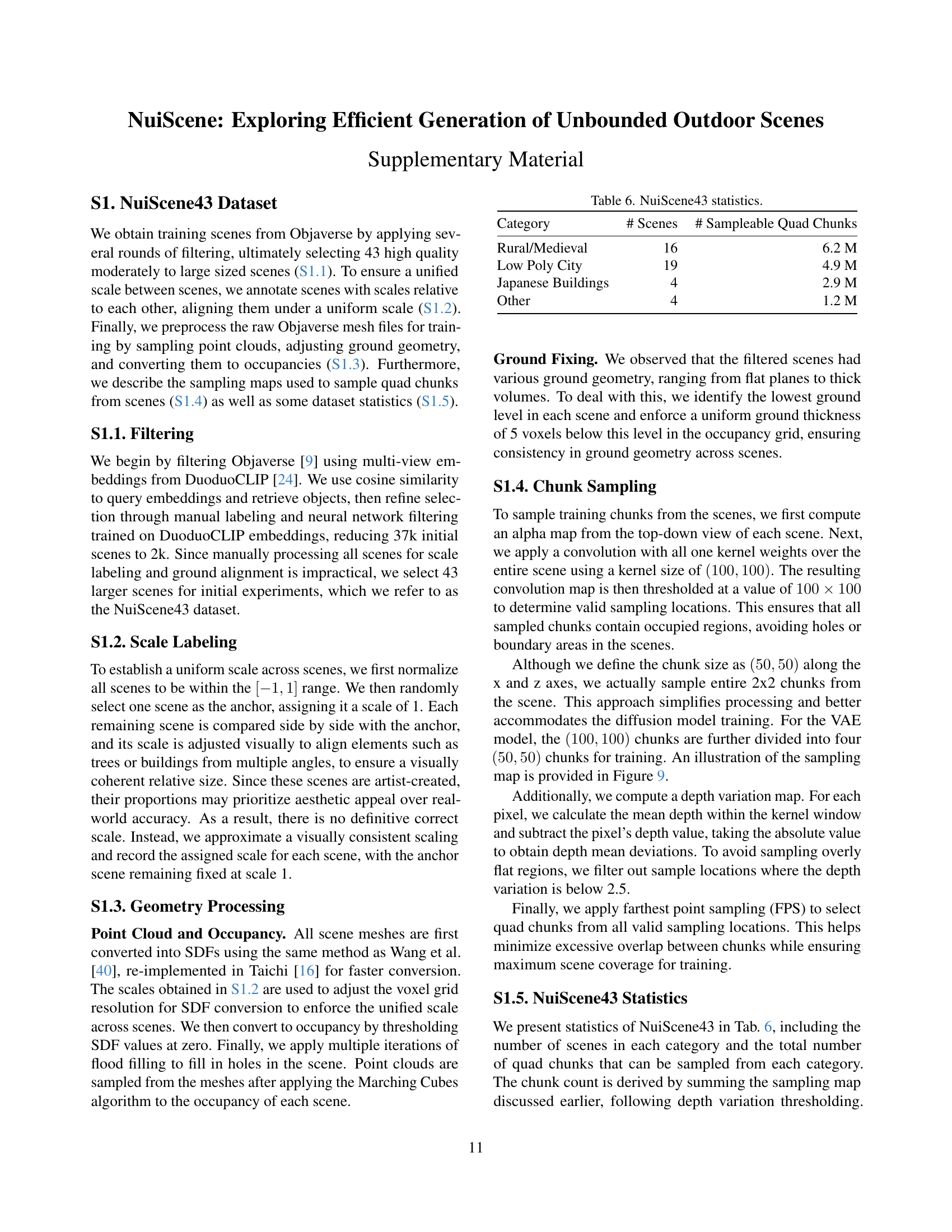
🔼 This table presents a statistical overview of the NuiScene43 dataset, which is a collection of 43 high-quality outdoor scenes used for training a model to generate unbounded outdoor scenes. The table breaks down the dataset by scene category (Rural/Medieval, Low Poly City, Japanese Buildings, Other), providing the number of scenes within each category and the total number of sampleable quad chunks available for training in each category. This information gives insight into the dataset’s composition and size, highlighting the diversity of scene types and the overall quantity of data available for model training.
read the caption
Table 6: NuiScene43 statistics.
Full paper#