TL;DR#
Diffusion models (DMs) are vital for generative modeling but computationally intensive, especially for high-resolution images. Existing acceleration methods often reduce sampling steps while overlooking data dimensionality. Recent work on next-scale prediction shows promise through gradually increasing resolution, resembling human perception. DMs still operate at a fixed dimensionality, leaving efficiency improvements unexplored. Therefore, a more effective approach to balance computational cost and performance is needed.
This paper introduces Scale-wise Distillation (SWD), a framework that generates images scale-by-scale across the diffusion process. SWD integrates into existing distillation methods and introduces a patch loss for finer similarity. Applied to text-to-image DMs, SWD achieves inference times of two full-resolution steps and outperforms counterparts with the same computation. It also competes or surpasses current text-to-image DMs with 2.5x-10x speed increase.
Key Takeaways#
Why does it matter?#
This paper introduces a novel and efficient approach to accelerate diffusion models, a cornerstone of modern generative AI, potentially impacting various applications by making high-quality image generation faster and more accessible.
Visual Insights#

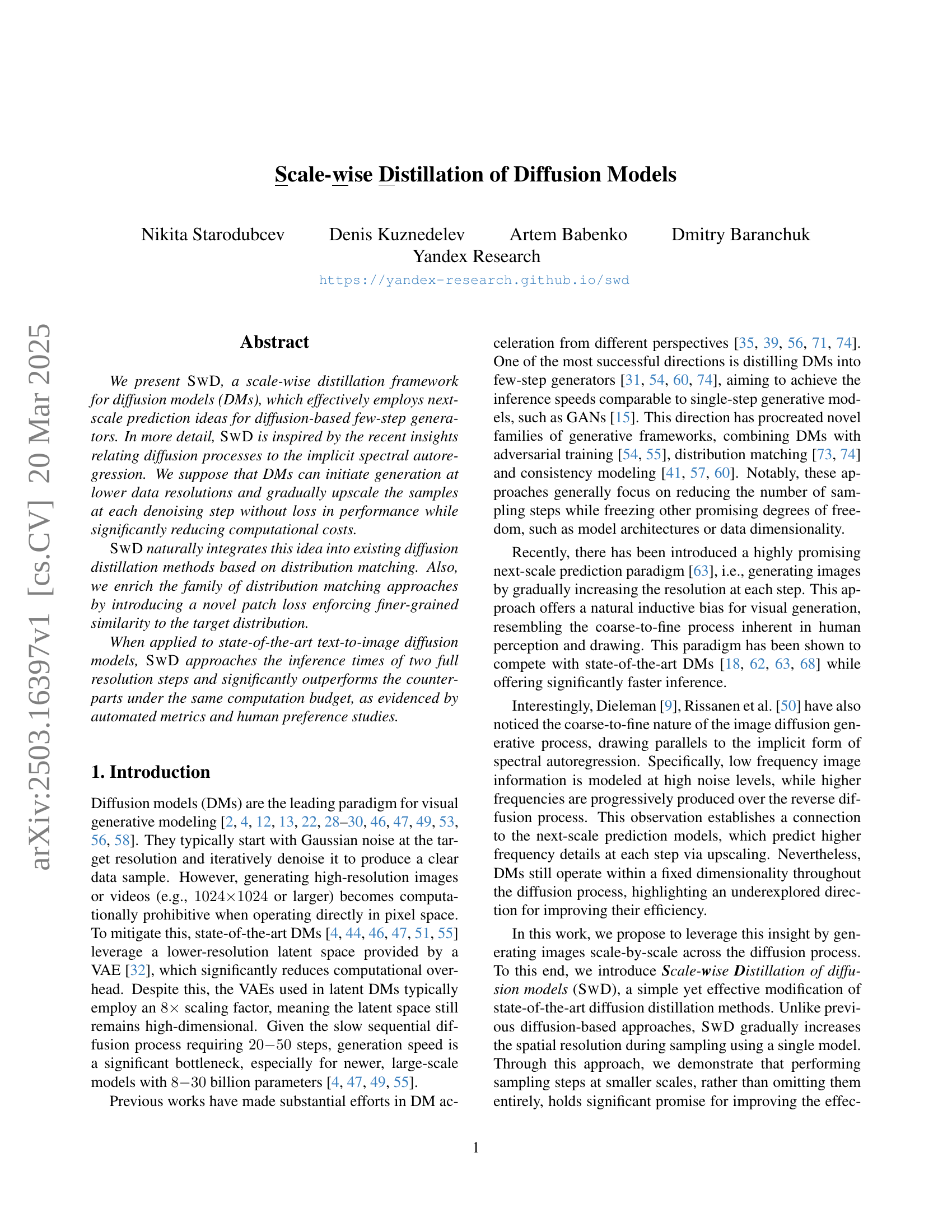
🔼 This figure displays the spectral analysis of SDXL and SD3.5 VAE latent spaces. The spectral density is shown for different diffusion timesteps. Vertical lines represent the frequency boundaries for lower resolution latent spaces (e.g., 16x16, 32x32, 96x96). Frequencies beyond these lines are not present at lower resolutions. The figure demonstrates that high frequencies are masked by noise at high noise levels. This observation supports the idea that latent diffusion models can efficiently operate at lower resolutions during the early stages of the diffusion process (i.e. at high noise levels).
read the caption
Figure 1: Spectral analysis of SDXL (Left) and SD3.5 (Right) VAE latents (128×128128128128{\times}128128 × 128) for different diffusion timesteps. Vertical lines mark frequency boundaries for lower resolutions; frequencies to the right are not present at lower scale latents. Noise masks high frequencies, suggesting that latent DMs can operate at lower latent resolutions for high noise levels.
| Configuration | |||
|---|---|---|---|
| A | |||
| B | |||
| C |
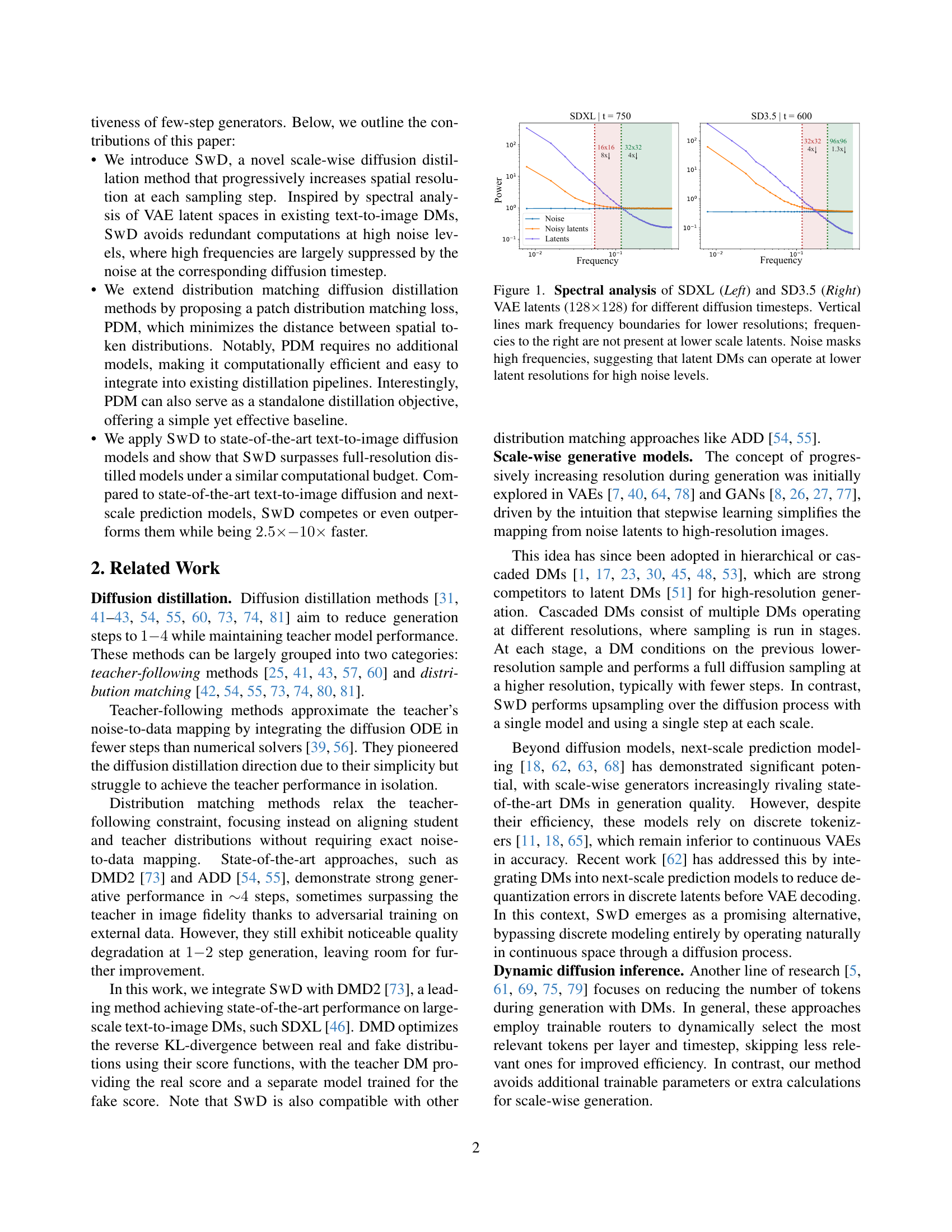
🔼 This table compares three different methods for upscaling noisy image latents from 64x64 to 128x128 resolution and then back down to 64x64. The goal is to determine which method produces upscaled latents that are most similar to the original full-resolution noisy latents. Method A uses the full resolution noisy latents as a baseline for comparison. Method B upscales the 64x64 latents and then adds noise. Method C adds noise to the 64x64 latents and then upscales. The similarity of the upscaled results to the original full-resolution noisy latents is measured using the Fréchet Inception Distance (FID), a metric used to evaluate the quality of generated images. The lower FID score indicates better quality. The table shows that Method B (upscaling first, then adding noise) produces upscaled latents that are closer to the ground truth full-resolution noisy latents than Method C (adding noise first, then upscaling).
read the caption
Table 1: Comparison of noisy latent upscaling strategies (B, C) for 64→128→6412864\rightarrow 12864 → 128 in terms of generation quality (FID-5K) against the real noisy latents (A). Upscaling 𝐱0downsubscriptsuperscript𝐱down0\mathbf{x}^{\text{down}}_{0}bold_x start_POSTSUPERSCRIPT down end_POSTSUPERSCRIPT start_POSTSUBSCRIPT 0 end_POSTSUBSCRIPT before noise injection (B) aligns better with full-resolution noisy latents.
In-depth insights#
Scale vs Quality#
The trade-off between scale and quality is a fundamental challenge in various domains, including image generation. In the context of diffusion models, increasing the scale, such as resolution, often leads to a higher computational cost and potentially slower generation times. Conversely, reducing the scale might improve speed but at the expense of image fidelity and detail. Achieving a balance between these factors requires careful consideration of model architecture, training strategies, and inference techniques. For instance, techniques like scale-wise distillation attempt to optimize this balance by generating images at lower resolutions initially and gradually increasing the resolution during the diffusion process. This approach can significantly reduce computational costs without sacrificing visual quality. A well-designed strategy can yield substantial performance gains, enabling faster and more efficient image generation.
SWD Mechanics#
Scale-wise Distillation (SWD) is a nuanced technique for diffusion models, leveraging the concept of progressively increasing image resolution during the denoising process. Instead of operating at a fixed resolution throughout, SWD begins at a lower resolution and gradually upscales the image, aiming to optimize computational efficiency without sacrificing quality. This approach draws inspiration from the spectral autoregression, which suggests that low-frequency information can be modeled at lower resolutions, making high-resolution processing unnecessary at early stages. The scale-wise approach requires careful consideration of when and how to perform upsampling; upscaling the clean latent representation before adding noise proves crucial for maintaining alignment with real noisy latents, addressing potential out-of-distribution issues. It also shifts time schedule for scale-wise generation by increasing time steps to address artifacts and upscales with bicubic interpolation. SWD’s architecture is also unique since it serves the dual purpose of few-shot generation and image upscaling.
Spectral Intuition#
While the term Spectral Intuition doesn’t explicitly appear, the research resonates with underlying spectral concepts. The document suggests that diffusion models implicitly perform spectral autoregression, aligning with Dieleman’s work. This implies that lower frequencies (coarse details) are modeled earlier in the diffusion process when noise is high, while higher frequencies (fine details) are gradually added as noise decreases. The study uses spectral analysis of latent spaces in VAEs and latent DMs. The data suggests that at high noise levels, high-frequency components are masked, allowing for operations at lower resolutions without significant information loss. Therefore high frequencies at timestep t are unnecessary if those frequencies are already masked at that noise level. This understanding is leveraged in SWD to avoid redundant computations. A next-scale prediction paradigm [63], i.e., generating images by gradually increasing the resolution at each step, offer natural inductive bias for visual generation. It is important that low resolution modeling in the proposed method does not lose any data signal.
Patch Matching Loss#
The idea of using a patch-matching loss is intriguing. Instead of focusing on the entire image, comparing smaller regions can lead to better local detail and texture matching. This approach can be especially useful when combined with other losses like adversarial loss, as it can help guide the generator towards creating more realistic and fine-grained structures. The use of intermediate features is also clever; it may enable the network to have access to more semantic level information for loss computation. Further exploration of different kernel choices and adaptive weighting of the patch loss based on image content or noise levels could prove valuable for enhancing the method’s overall effectiveness and robustness. Specifically, RBF kernel might improve image quality.
Adaptive Scales#
The idea of adaptive scales in diffusion models presents a compelling avenue for optimizing computational efficiency and potentially improving generative quality. Instead of adhering to a fixed resolution throughout the entire diffusion process, an adaptive approach would dynamically adjust the scale of operations based on factors such as noise levels, timestep, or content complexity. During the initial high-noise timesteps, lower resolutions could be employed to capture the coarse, low-frequency structures of the data distribution, leading to significant computational savings. As the diffusion process progresses and noise decreases, the resolution could be gradually increased to refine finer details. Adaptive scales could be implemented using various techniques, such as dynamic pooling, wavelet transformations, or hierarchical representations. Challenges include designing effective scale-selection mechanisms, ensuring smooth transitions between scales, and maintaining consistency across different resolutions. However, the potential benefits in terms of speed, memory usage, and potentially even improved generation make it a worthwhile research direction.
More visual insights#
More on figures

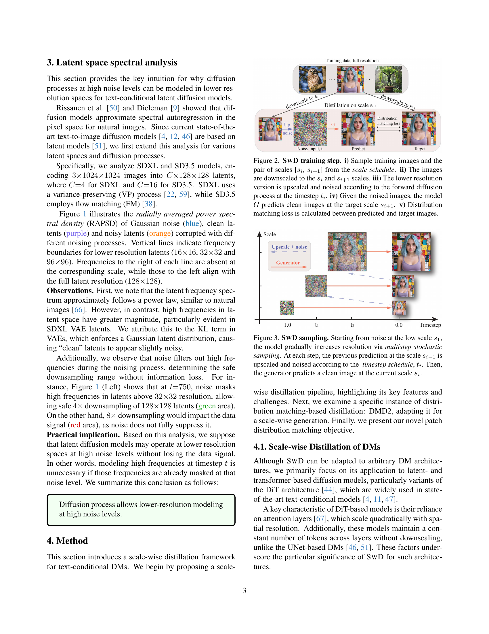
🔼 The figure illustrates the training process of the Scale-wise Distillation (SWD) method. It’s a five-step process: 1) Select a training image and a pair of scales (si and si+1) from a predefined scale schedule. 2) Downscale the image to both si and si+1 resolutions. 3) Upscale the lower-resolution (si) image and add noise according to the forward diffusion process at timestep ti. 4) The model G predicts a clean image at the target scale si+1. 5) Finally, calculate the distribution matching loss between the model’s prediction and the original, target image at scale si+1. This loss guides the training of model G to accurately predict images at higher resolutions by progressively upscaling and denoising.
read the caption
Figure 2: SwD training step. i) Sample training images and the pair of scales [sisubscript𝑠𝑖s_{i}italic_s start_POSTSUBSCRIPT italic_i end_POSTSUBSCRIPT, si+1subscript𝑠𝑖1s_{i+1}italic_s start_POSTSUBSCRIPT italic_i + 1 end_POSTSUBSCRIPT] from the scale schedule. ii) The images are downscaled to the sisubscript𝑠𝑖s_{i}italic_s start_POSTSUBSCRIPT italic_i end_POSTSUBSCRIPT and si+1subscript𝑠𝑖1s_{i+1}italic_s start_POSTSUBSCRIPT italic_i + 1 end_POSTSUBSCRIPT scales. iii) The lower resolution version is upscaled and noised according to the forward diffusion process at the timestep tisubscript𝑡𝑖t_{i}italic_t start_POSTSUBSCRIPT italic_i end_POSTSUBSCRIPT. iv) Given the noised images, the model G𝐺Gitalic_G predicts clean images at the target scale si+1subscript𝑠𝑖1s_{i+1}italic_s start_POSTSUBSCRIPT italic_i + 1 end_POSTSUBSCRIPT. v) Distribution matching loss is calculated between predicted and target images.

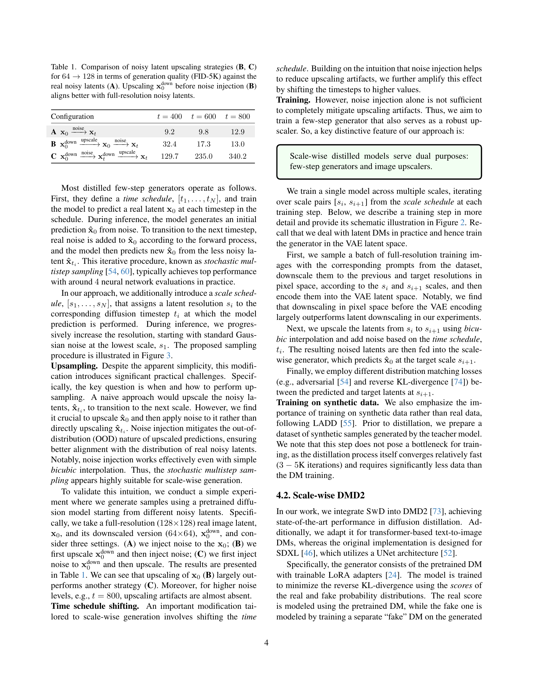
🔼 This figure illustrates the SWD (Scale-wise Distillation) sampling process. It starts with pure Gaussian noise at a low initial resolution (s1). The model then iteratively refines this noisy image through multiple steps. In each step, the model upscales the previous prediction to a higher resolution (si) and adds noise according to a predefined timestep schedule (ti). This noisy image is then fed to the generator, which outputs a progressively cleaner, higher-resolution prediction at each step, until the final, high-resolution image is produced. The process mimics a coarse-to-fine approach, starting with low-frequency details at lower resolutions and gradually adding high-frequency details at each step.
read the caption
Figure 3: SwD sampling. Starting from noise at the low scale s1subscript𝑠1s_{1}italic_s start_POSTSUBSCRIPT 1 end_POSTSUBSCRIPT, the model gradually increases resolution via multistep stochastic sampling. At each step, the previous prediction at the scale si−1subscript𝑠𝑖1s_{i-1}italic_s start_POSTSUBSCRIPT italic_i - 1 end_POSTSUBSCRIPT is upscaled and noised according to the timestep schedule, tisubscript𝑡𝑖t_{i}italic_t start_POSTSUBSCRIPT italic_i end_POSTSUBSCRIPT. Then, the generator predicts a clean image at the current scale sisubscript𝑠𝑖s_{i}italic_s start_POSTSUBSCRIPT italic_i end_POSTSUBSCRIPT.

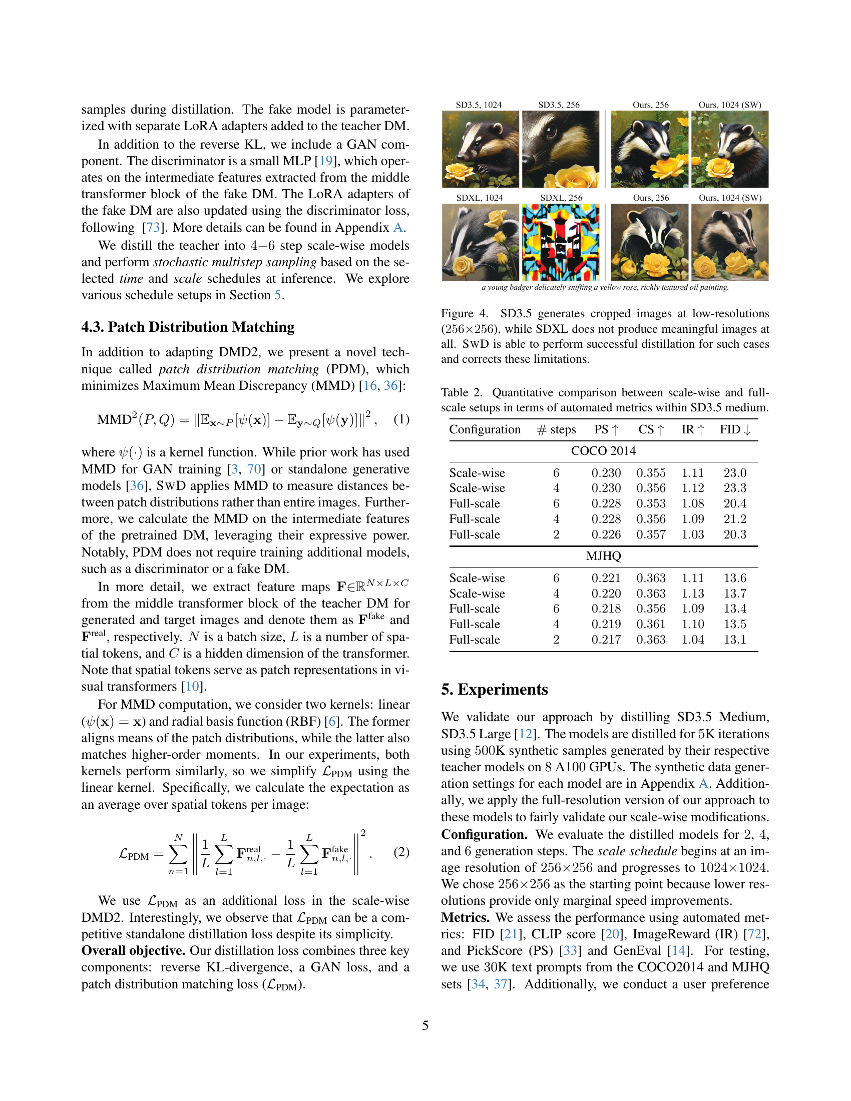
🔼 This figure demonstrates the impact of using a scale-wise distillation method (SwD) compared to training at full resolution. At a lower resolution (256x256), SD3.5, a diffusion model, produces cropped images lacking detail. SDXL, another diffusion model, fails to generate coherent images at this resolution. However, SwD successfully distills these models, generating more complete and higher quality images. This highlights the SwD’s ability to correct the limitations found in models trained at higher resolutions for lower-resolution tasks.
read the caption
Figure 4: SD3.5 generates cropped images at low-resolutions (256×256256256256{\times}256256 × 256), while SDXL does not produce meaningful images at all. SwD is able to perform successful distillation for such cases and corrects these limitations.

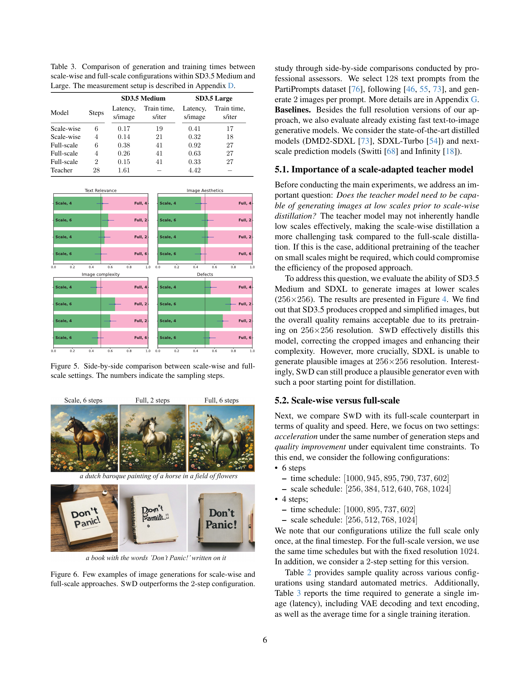
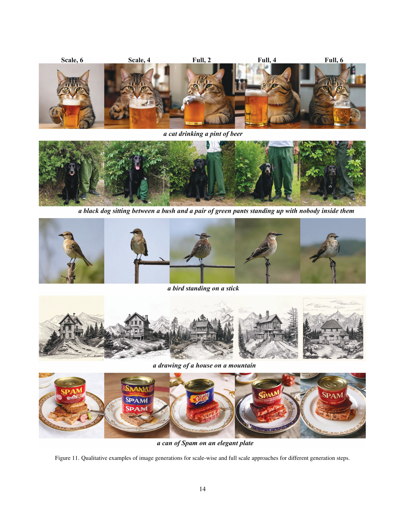
🔼 This figure presents a visual comparison of image generation results using scale-wise and full-scale methods for different numbers of sampling steps. It helps to illustrate the effectiveness of the scale-wise approach, which progressively increases the image resolution during generation, in comparison to the traditional full-scale method. The images generated by both methods across varying numbers of steps are presented side-by-side for comparison. The number of steps used for generation is indicated below each set of images, enabling a direct visual analysis of how image quality changes with the number of steps and the chosen method.
read the caption
Figure 5: Side-by-side comparison between scale-wise and full-scale settings. The numbers indicate the sampling steps.

🔼 Figure 6 presents a comparison of image generation results between the scale-wise distillation method (SWD) and the full-scale method. It showcases several example prompts and their corresponding generated images. The images highlight the improved quality and detail achieved by SWD, especially when compared to the full-scale method with only two steps. The scale-wise approach produces more coherent and detailed images, demonstrating its superiority over the faster but less accurate full-scale approach.
read the caption
Figure 6: Few examples of image generations for scale-wise and full-scale approaches. SwD outperforms the 2222-step configuration.

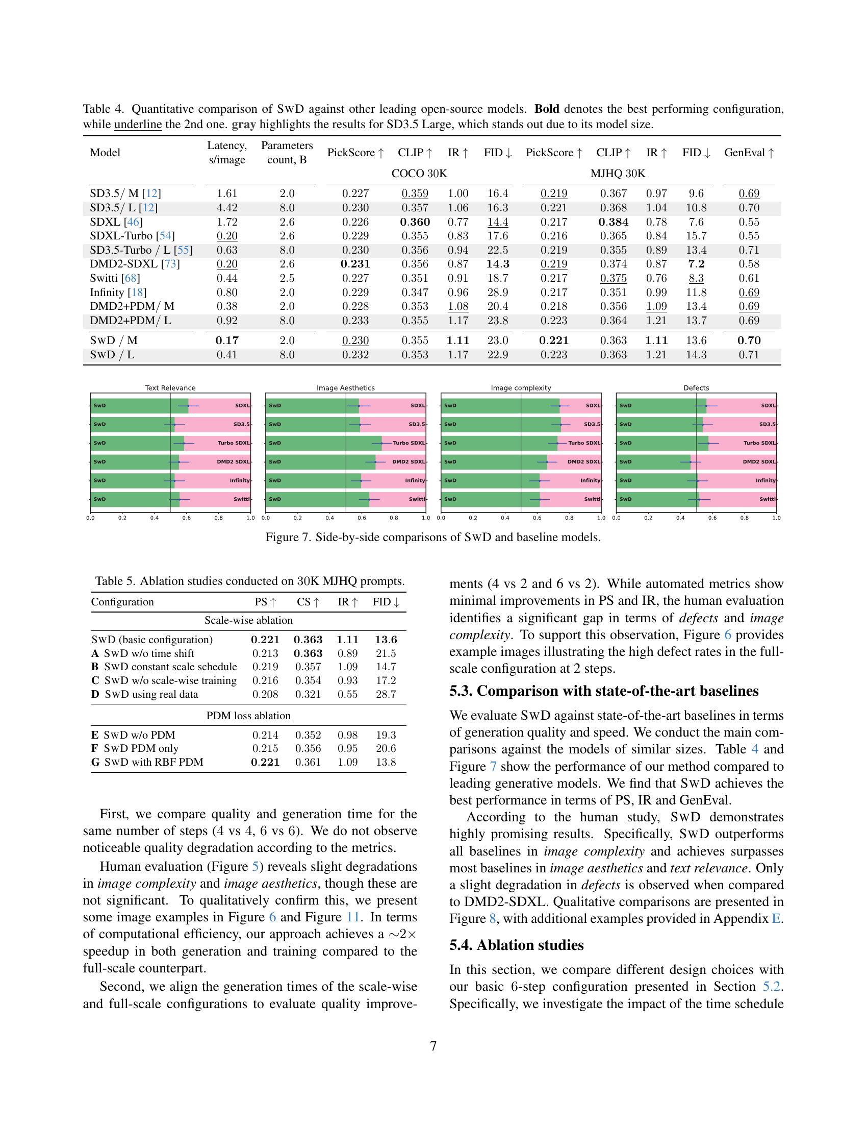
🔼 This figure presents a side-by-side comparison of the generated images from SwD and several baseline models, across four key aspects: text relevance, image aesthetics, image complexity, and defects. For each metric, the figure shows bar graphs representing the human evaluation scores for SwD and the baselines, enabling a visual comparison of their relative performance in these criteria. This allows for a quick assessment of SwD’s strengths and weaknesses when compared to state-of-the-art methods.
read the caption
Figure 7: Side-by-side comparisons of SwD and baseline models.

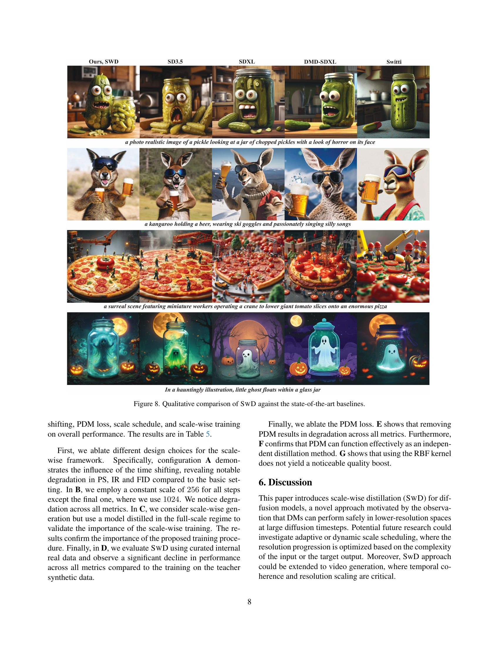
🔼 Figure 8 presents a qualitative comparison of image generation results between the proposed Scale-wise Distillation (SwD) method and several state-of-the-art baselines. Four example image prompts are shown, with each showing the output of SwD and the outputs of the baselines. This allows for a visual comparison of the image quality, detail, and overall fidelity across different methods, highlighting the strengths and weaknesses of each in terms of generating high-quality, detailed images.
read the caption
Figure 8: Qualitative comparison of SwD against the state-of-the-art baselines.

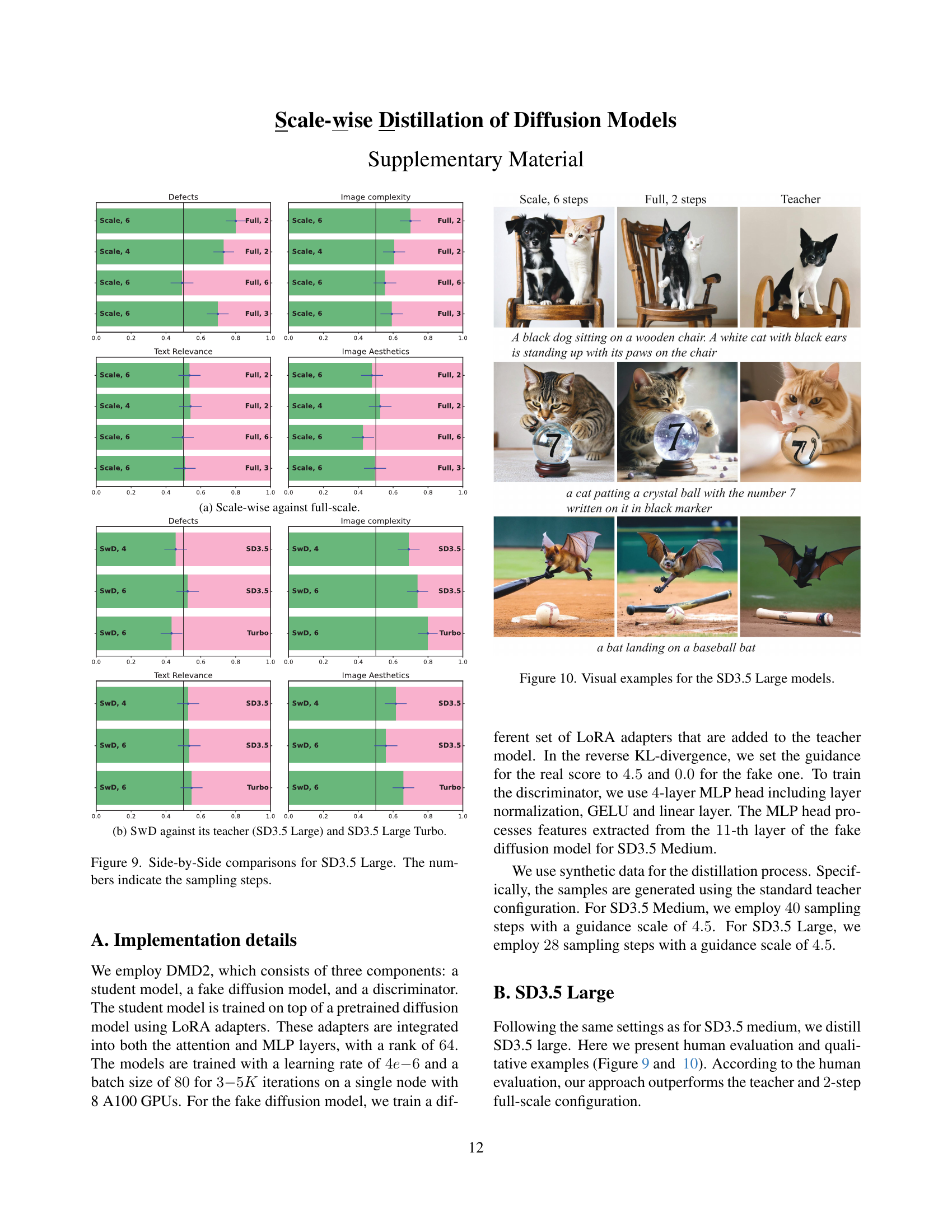
🔼 This figure shows a comparison of the scale-wise approach against the full-scale approach. Specifically, it presents a visual comparison of the results obtained by using the scale-wise method (progressively increasing the resolution at each sampling step) versus the full-resolution method. The comparison allows assessment of the tradeoffs between computational efficiency and image quality using the two approaches.
read the caption
(a) Scale-wise against full-scale.
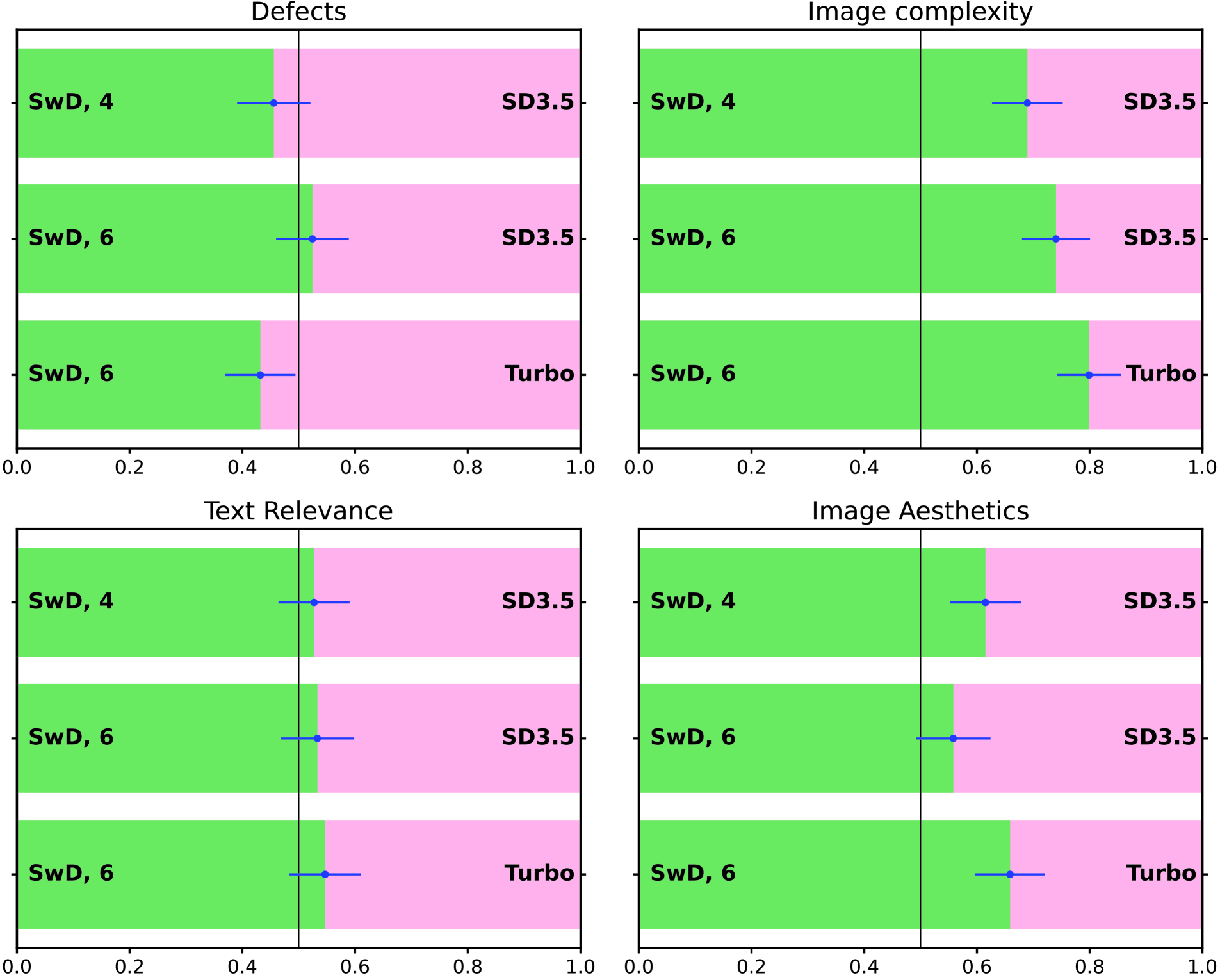
🔼 This figure presents a comparison of the performance of SwD against its teacher model (SD3.5 Large) and a state-of-the-art, fast text-to-image diffusion model (SD3.5 Large Turbo). The comparison is conducted using human evaluation across multiple criteria, namely image aesthetics, text relevance, image complexity, and defects. The results visualize the relative strengths and weaknesses of SwD concerning these aspects compared to existing models, illustrating how well SwD manages to preserve or improve upon its teacher’s performance while offering a significant speedup.
read the caption
(b) SwD against its teacher (SD3.5 Large) and SD3.5 Large Turbo.

🔼 This figure shows a comparison of the image quality generated by different models: the full-resolution SD3.5 Large model and its scale-wise distilled counterparts with 4 and 6 sampling steps. The images generated from each model are presented side-by-side, allowing for visual comparison of the image quality and detail. The results are further assessed using human evaluations on various aspects like text relevance, image aesthetics, complexity, and presence of defects. This comparison helps to demonstrate the effectiveness of the scale-wise distillation method.
read the caption
Figure 9: Side-by-Side comparisons for SD3.5 Large. The numbers indicate the sampling steps.

🔼 This figure showcases visual examples generated by SD3.5 Large models, highlighting the diverse range of image styles and subject matters achievable using the model. The examples illustrate the model’s capacity to create a variety of images given different prompts.
read the caption
Figure 10: Visual examples for the SD3.5 Large models.

🔼 This figure showcases several image generation examples using both scale-wise and full-scale approaches with varying generation steps (2, 4, and 6 steps). Each row represents a different text prompt, and the images within each row demonstrate the results from different methods and step counts. This allows for a visual comparison of the image quality and detail achieved by each approach. The purpose is to highlight the qualitative differences between the scale-wise distillation technique and a more traditional full-scale approach with different numbers of sampling steps, demonstrating the capabilities of the proposed method in producing high-quality images with fewer steps.
read the caption
Figure 11: Qualitative examples of image generations for scale-wise and full scale approaches for different generation steps.

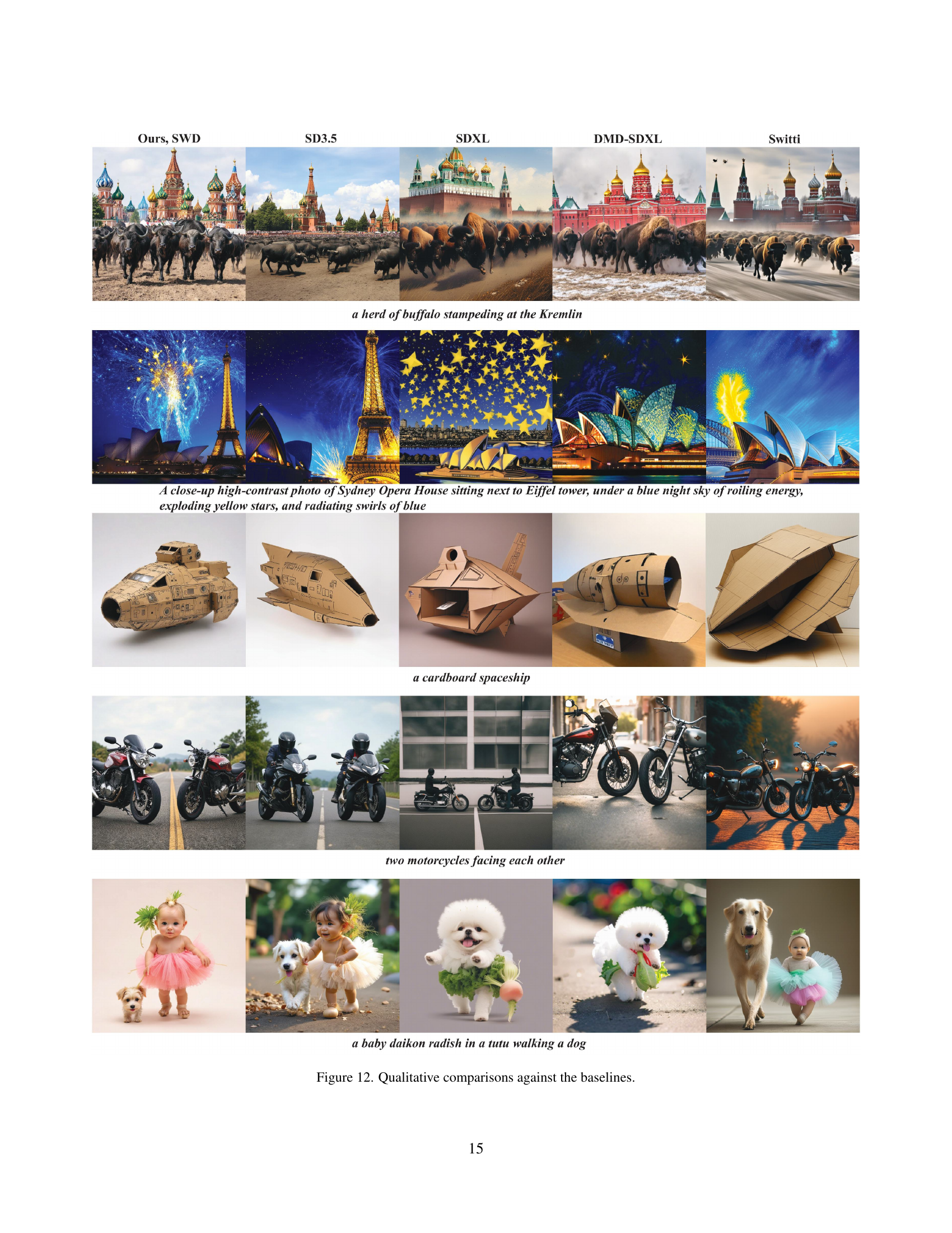
🔼 This figure shows a qualitative comparison of image generation results from various models, including the proposed Scale-wise Distillation of Diffusion Models (SWD) and several state-of-the-art baselines (SD3.5, SDXL, DMD-SDXL, and Switti). For each model, several image examples are displayed for the same text prompt, allowing for a visual comparison of image quality, detail, realism, and adherence to the prompt. This side-by-side comparison helps highlight the strengths and weaknesses of SWD compared to other methods.
read the caption
Figure 12: Qualitative comparisons against the baselines.

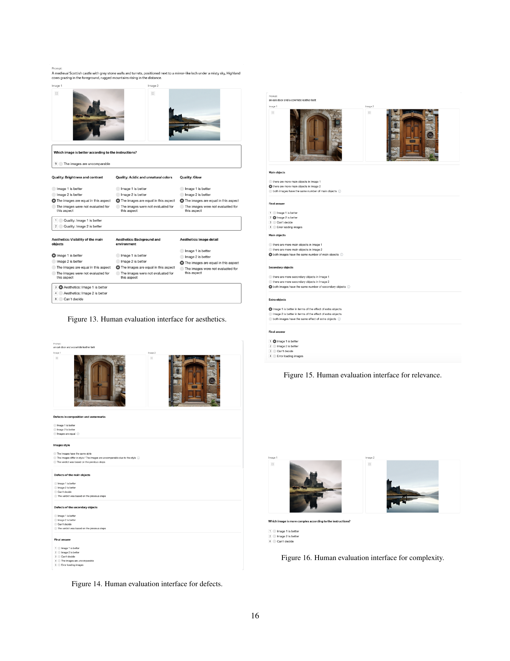
🔼 This figure shows the user interface used for human evaluation of image aesthetics. Assessors are presented with pairs of images and asked to compare them based on several criteria, including brightness and contrast, color quality, glow, visibility of main objects, background and environment, and level of detail in the images. A multiple choice format allows assessors to indicate which image is better or if they are comparable in quality for a given criterion. The final rating is a consolidated judgment across all the criteria.
read the caption
Figure 13: Human evaluation interface for aesthetics.

🔼 This figure displays the interface used by assessors in the human evaluation study. Assessors are presented with a pair of images and asked to evaluate the presence of defects. The interface guides assessors through specific types of defects such as those in composition, watermarks, or extra objects. Assessors rate images based on the severity of these defects and provide a final decision for each image pair.
read the caption
Figure 14: Human evaluation interface for defects.

🔼 This figure shows the interface used by human evaluators to assess the relevance of generated images to the given text prompt. The evaluators are presented with a pair of images and asked to judge which image is more relevant to the prompt, considering aspects like the main objects and secondary objects depicted. They also assess the impact of any extra objects present in the image and provide a final verdict indicating which image demonstrates better relevance.
read the caption
Figure 15: Human evaluation interface for relevance.
More on tables
| Configuration | steps | PS | CS | IR | FID |
|---|---|---|---|---|---|
| COCO 2014 | |||||
| Scale-wise | |||||
| Scale-wise | |||||
| Full-scale | |||||
| Full-scale | |||||
| Full-scale | |||||
| MJHQ | |||||
| Scale-wise | |||||
| Scale-wise | |||||
| Full-scale | |||||
| Full-scale | |||||
| Full-scale | |||||
🔼 This table presents a quantitative comparison of the performance of scale-wise and full-scale diffusion models using several automated metrics. Specifically, it shows the results for the SD3.5 medium model, comparing different numbers of sampling steps (2, 4, and 6 steps) for both scale-wise and full-scale approaches. The metrics used include FID (Fréchet Inception Distance), which measures the quality of generated images, as well as PS (PickScore), CS (CLIPScore), and IR (ImageReward), all reflecting different aspects of image quality and similarity to the desired output.
read the caption
Table 2: Quantitative comparison between scale-wise and full-scale setups in terms of automated metrics within SD3.5 medium.
| SD3.5 Medium | SD3.5 Large | |||||||||||||
|---|---|---|---|---|---|---|---|---|---|---|---|---|---|---|
| Model | Steps |
|
|
|
| |||||||||
| Scale-wise | ||||||||||||||
| Scale-wise | ||||||||||||||
| Full-scale | ||||||||||||||
| Full-scale | ||||||||||||||
| Full-scale | ||||||||||||||
| Teacher | ||||||||||||||
🔼 This table presents a quantitative comparison of the generation and training times for scale-wise and full-scale diffusion models. It compares two different model sizes (SD3.5 Medium and SD3.5 Large) across various numbers of sampling steps (2, 4, and 6). The data highlights the computational efficiency gains achieved by using the scale-wise approach, showing significant reductions in both generation and training times compared to the full-resolution methods. Details on the experimental setup can be found in Appendix D of the paper.
read the caption
Table 3: Comparison of generation and training times between scale-wise and full-scale configurations within SD3.5 Medium and Large. The measurement setup is described in Appendix D.
| Latency, |
| s/image |
🔼 This table presents a quantitative comparison of the proposed Scale-wise Distillation (SwD) method against other state-of-the-art open-source text-to-image generation models. The comparison is based on several key metrics: generation speed (Latency), model size (Parameters), and image quality (evaluated using PickScore, CLIP score, Inception score, FID, and GenEval). The table highlights the best-performing configuration for each model and uses bold text to emphasize the top performer and underlines to indicate the second-best. Results for the larger SD3.5 Large model are shown in gray to emphasize the model size’s impact on the results.
read the caption
Table 4: Quantitative comparison of SwD against other leading open-source models. Bold denotes the best performing configuration, while underline the 2nd one. gray highlights the results for SD3.5 Large, which stands out due to its model size.
| Train time, |
| s/iter |
🔼 This table presents the results of ablation studies conducted on 30K MJHQ prompts to analyze the impact of different components of the proposed Scale-wise Distillation of Diffusion Models (SWD) method. The studies systematically remove or modify specific parts of the SWD framework (e.g., time shifting, scale scheduling, scale-wise training, the Patch Distribution Matching loss (PDM)) to isolate their individual contributions to the overall performance. The table shows the impact of each ablation on standard metrics: PS↑ (PickScore), CS↑ (CLIPScore), IR↑ (ImageReward), and FID↓ (Fréchet Inception Distance). The results help to understand the relative importance of different components of the SWD method.
read the caption
Table 5: Ablation studies conducted on 30303030K MJHQ prompts.
| Latency, |
| s/image |
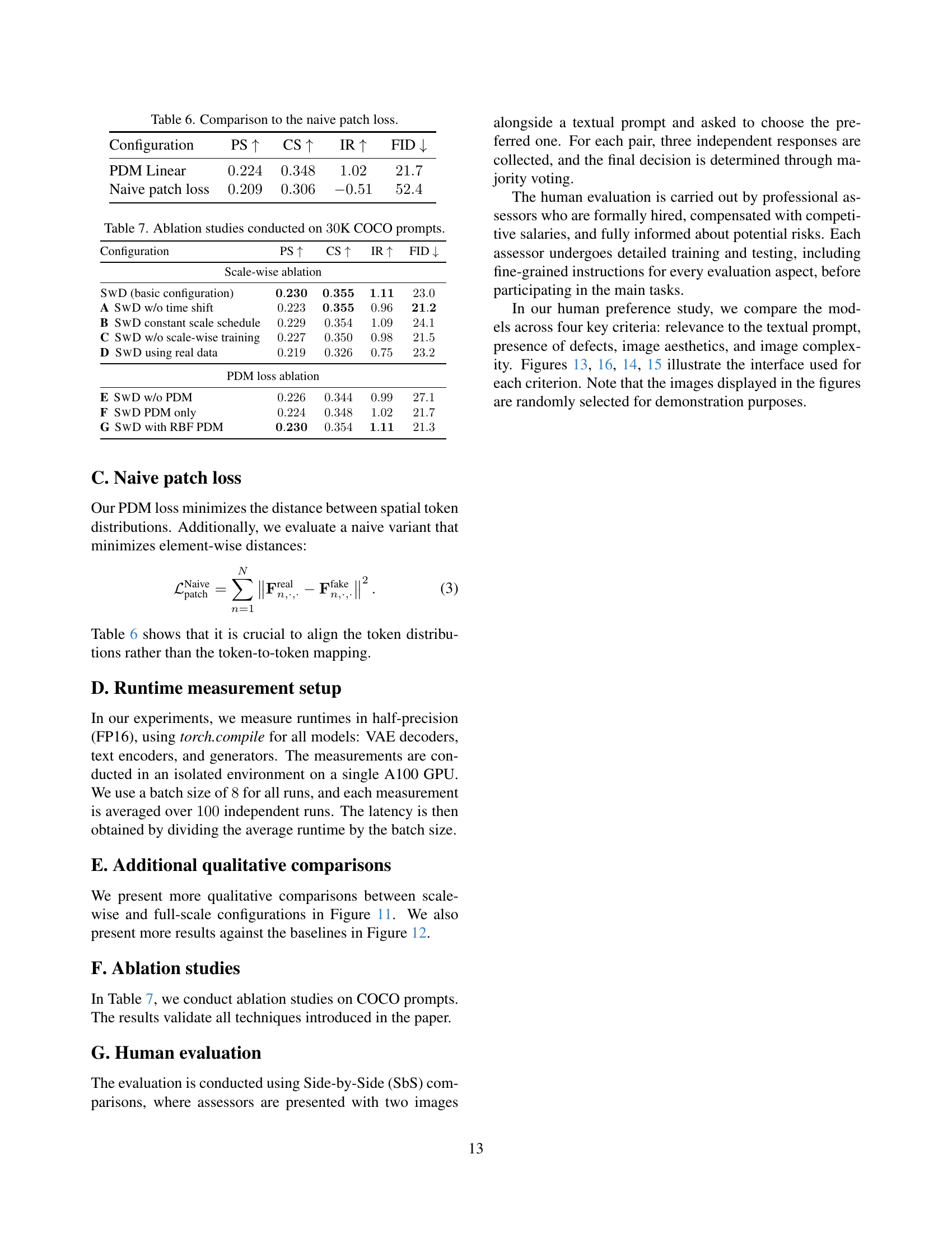
🔼 This table compares the performance of the proposed Patch Distribution Matching (PDM) loss with a naive patch loss. The naive patch loss simply calculates the element-wise distance between patches in the feature maps from the teacher and student models. PDM uses the Maximum Mean Discrepancy (MMD) to measure the distance between patch distributions, providing a more robust and informative comparison of the patch similarity. The table shows the results in terms of PS (PickScore), CS (CLIP Score), IR (ImageReward), and FID (Frechet Inception Distance) metrics on the COCO 2014 dataset. The results demonstrate the superiority of PDM over the naive patch loss in terms of image quality and generation performance.
read the caption
Table 6: Comparison to the naive patch loss.
| Train time, |
| s/iter |
🔼 This table presents the results of ablation studies performed on the COCO dataset to analyze the impact of different components of the proposed Scale-wise Distillation of Diffusion Models (SWD) method. The studies systematically remove or modify key elements of SWD, such as the time shift, scale schedule, training method, and the Patch Distribution Matching (PDM) loss, to evaluate their individual contributions to the overall performance. The metrics used to assess performance include PS (PickScore), CS (CLIPScore), IR (ImageReward), and FID (Fréchet Inception Distance). This analysis helps to understand the importance of each component and identify potential areas for improvement or simplification of the SWD framework.
read the caption
Table 7: Ablation studies conducted on 30303030K COCO prompts.
Full paper#