TL;DR#
4D Gaussian Splatting (4DGS) has emerged for dynamic scene reconstruction. Current 4DGS methods require substantial storage and suffer from slow rendering speed. This paper identifies two key sources of temporal redundancy. First, many Gaussians have short lifespans, leading to excessive numbers. Second, only a subset of Gaussians contributes to each frame, yet all are processed during rendering. The goal is to compress 4DGS by reducing the number of Gaussians while preserving rendering quality.
To address these issues, the paper introduces 4DGS-1K, running at over 1000 FPS. The proposed method introduces the Spatial-Temporal Variation Score, a new pruning criterion that removes short-lifespan Gaussians while encouraging longer temporal spans. The paper also stores a mask for active Gaussians across consecutive frames, reducing redundant computations. Compared to vanilla 4DGS, 4DGS-1K achieves a 41× reduction in storage and 9× faster rasterization speed, maintaining visual quality.
Key Takeaways#
Why does it matter?#
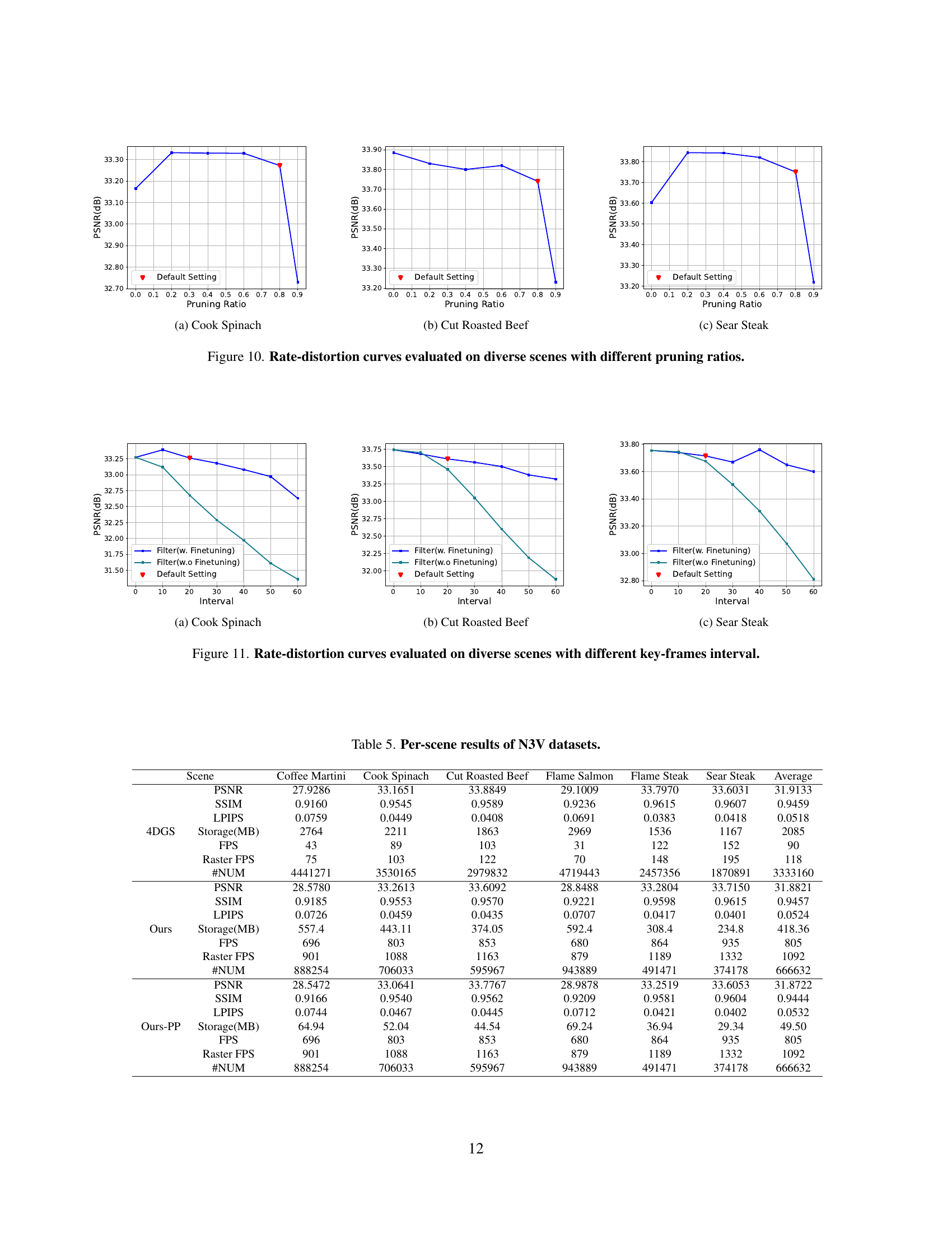
This paper is crucial for advancing dynamic scene rendering, offering a practical solution to overcome the limitations of 4DGS. By significantly reducing storage and improving rendering speed, it enables more efficient and accessible real-time applications. It also presents new directions for future research, focusing on developing universal compression methods and optimizing rendering modules.
Visual Insights#

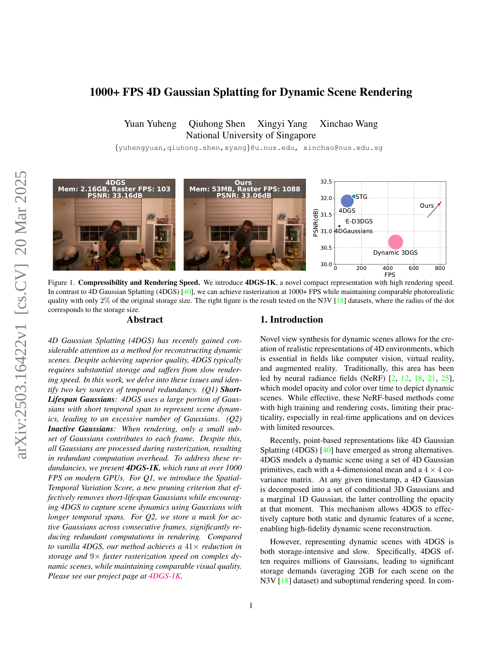
🔼 Figure 1 demonstrates the improved performance of the proposed 4DGS-1K method compared to the existing 4D Gaussian Splatting (4DGS). The left side shows a qualitative comparison of the reconstruction results between the two methods. 4DGS-1K achieves comparable photorealistic quality with a significantly faster rasterization speed (1000+ FPS) and only requires 2% of the original storage size. The right side presents a quantitative comparison in terms of PSNR versus the rendering speed, tested on the N3V dataset. The size of the dots represents the storage size, clearly showing the advantage of the 4DGS-1K method.
read the caption
Figure 1: Compressibility and Rendering Speed. We introduce 4DGS-1K, a novel compact representation with high rendering speed. In contrast to 4D Gaussian Splatting (4DGS) [40], we can achieve rasterization at 1000+ FPS while maintaining comparable photorealistic quality with only 2%percent22\%2 % of the original storage size. The right figure is the result tested on the N3V [18] datasets, where the radius of the dot corresponds to the storage size.
| Method | PSNR | SSIM | LPIPS | Storage(MB) | FPS | Raster FPS | #Gauss |
| Neural Volume1[21] | 22.80 | - | 0.295 | - | - | - | - |
| DyNeRF1[18] | 29.58 | - | 0.083 | 28 | 0.015 | - | - |
| StreamRF[17] | 28.26 | - | - | 5310 | 10.90 | - | - |
| HyperReel[2] | 31.10 | 0.927 | 0.096 | 360 | 2.00 | - | - |
| K-Planes[12] | 31.63 | - | 0.018 | 311 | 0.30 | - | - |
| Dynamic 3DGS[23] | 30.67 | 0.930 | 0.099 | 2764 | 460 | - | - |
| 4DGaussian[39] | 31.15 | 0.940 | 0.049 | 90 | 30 | - | - |
| E-D3DGS[3] | 31.31 | 0.945 | 0.037 | 35 | 74 | - | - |
| STG[19] | 32.05 | 0.946 | 0.044 | 200 | 140 | - | - |
| 4D-RotorGS[7] | 31.62 | 0.940 | 0.140 | - | 277 | - | - |
| MEGA[43] | 31.49 | - | 0.056 | 25 | 77 | - | - |
| Compact3D[16] | 31.69 | 0.945 | 0.054 | 15 | 186 | - | - |
| 4DGS[40] | 32.01 | - | 0.055 | - | 114 | - | - |
| 4DGS2[40] | 31.91 | 0.946 | 0.052 | 2085 | 90 | 118 | 3333160 |
| Ours | 31.88 | 0.946 | 0.052 | 418 | 805 | 1092 | 666632 |
| Ours-PP | 31.87 | 0.944 | 0.053 | 50 | 805 | 1092 | 666632 |
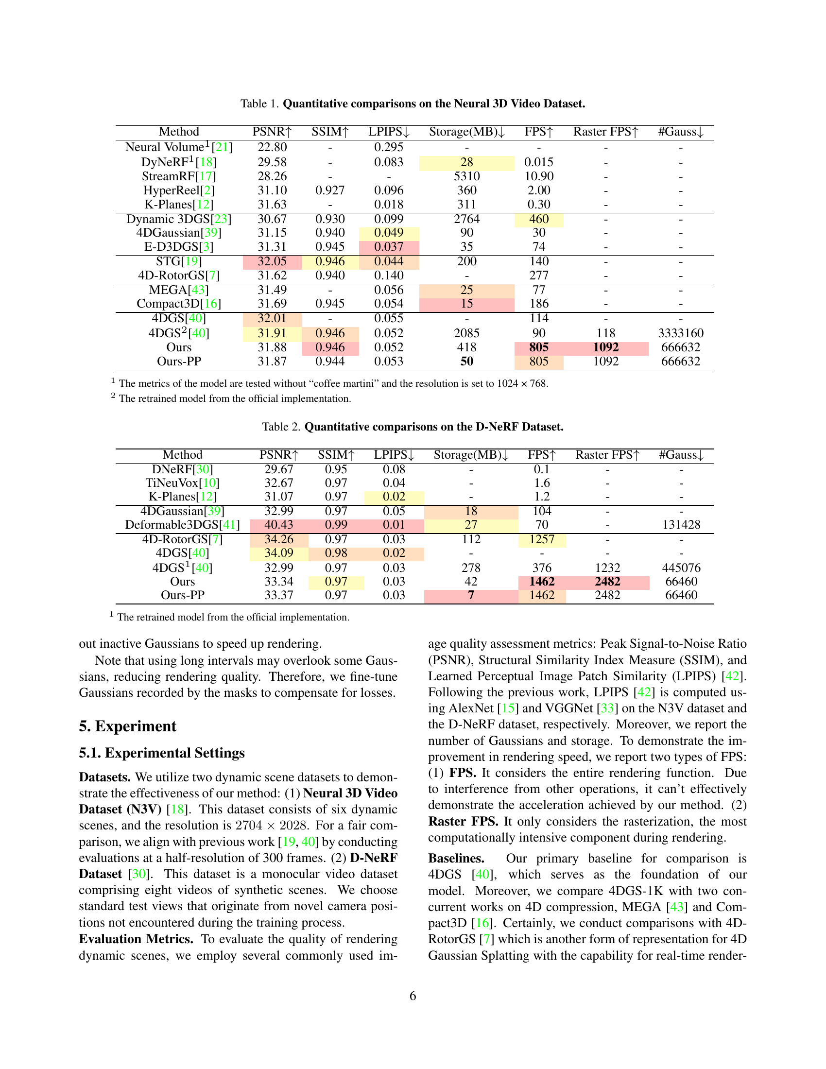
🔼 This table presents a quantitative comparison of different methods for novel view synthesis on the Neural 3D Video dataset. Metrics include Peak Signal-to-Noise Ratio (PSNR), Structural Similarity Index Measure (SSIM), Learned Perceptual Image Patch Similarity (LPIPS), storage size in MB, rendering speed in frames per second (FPS), rasterization speed in FPS, and the number of Gaussian primitives used. The table allows for a direct comparison of the performance and efficiency of various approaches in reconstructing dynamic scenes.
read the caption
Table 1: Quantitative comparisons on the Neural 3D Video Dataset.
In-depth insights#
4DGS Redundancy#
The 4DGS redundancy stems from inefficient representation of dynamic scenes, leading to high storage and slow rendering. The paper identifies short-lifespan Gaussians which flicker briefly, and inactive Gaussians processed unnecessarily. These redundancies suggest a need for compression techniques focusing on pruning transient Gaussians and filtering inactive ones to improve efficiency without compromising quality. Addressing temporal redundancy is crucial for optimizing 4DGS. This involves leveraging temporal coherence and minimizing redundant Gaussian primitives. A compact, memory-efficient framework is essential to deal with these issues.
Spatial-Temporal#
The concept of ‘Spatial-Temporal’ is crucial for understanding dynamic scenes, as it combines spatial information with temporal evolution. Representations that model both space and time effectively can capture complex motions and changes in a scene. This is particularly relevant in dynamic scene rendering, where the goal is to generate realistic images from novel viewpoints at different points in time. A key challenge lies in efficiently representing this 4D data, often requiring significant storage and computational resources. Methods that leverage spatial-temporal coherence, such as sharing information across adjacent frames, can reduce redundancy and improve performance. The analysis of spatial-temporal variations can guide the pruning of less important elements, leading to more compact and efficient representations without sacrificing visual quality. Accurately modeling spatial-temporal relationships is essential for applications like virtual reality, augmented reality, and autonomous navigation.
Inactive Pruning#
Inactive Gaussian pruning is crucial for efficient dynamic scene rendering, addressing the redundancy in 4D Gaussian Splatting (4DGS). The core idea is to identify and remove Gaussians that contribute negligibly to the final rendered image at each frame. This is motivated by the observation that, at any given time, only a small subset of Gaussians are ‘active,’ while the rest remain inactive, leading to wasted computations. Effective pruning strategies are thus necessary to accelerate rendering without compromising quality. This may include using key-frame temporal filter by sharing masks for adjacent frames based on observation that Gaussians are active. By decreasing computations on inactive parts, the method can improve the rendering speed.
1K+FPS Rendering#
Achieving 1K+ FPS rendering is a significant leap in dynamic scene representation, particularly with Gaussian Splatting. This advancement addresses the prior limitations of methods like 4DGS, which struggled with both storage intensity and slow rendering speeds. The core strategy involves minimizing redundancy, focusing on two key areas. First, pruning short-lifespan Gaussians to reduce overall count, and second, filtering inactive Gaussians to decrease per-frame computational load. This optimization not only makes the representation more compact but also dramatically accelerates the rendering process. The implications are far-reaching, enabling real-time applications and deployment on devices with limited resources, marking a critical step towards practical, high-fidelity dynamic scene modeling. The ability to achieve such high frame rates while maintaining comparable photorealistic quality highlights the efficiency of the proposed techniques in addressing both storage and computational bottlenecks, paving the way for more accessible and versatile dynamic scene rendering solutions.
Mask Refinement#
Mask refinement is crucial for precise object segmentation in dynamic scenes. The initial masks generated may be coarse, and refining them enhances accuracy for downstream tasks. Techniques could involve morphological operations to smooth boundaries and fill gaps. Also, consider conditional random fields to enforce spatial consistency with neighboring pixels. Temporal information could be integrated to track object motion and refine masks across frames. This ensures the masks are aligned with the actual object boundaries and the visual context, especially where lighting or shadows can affect mask boundaries.
More visual insights#
More on figures

🔼 This figure shows the distribution of the temporal variance parameter (Στ) for all Gaussians in the Sear Steak scene. The x-axis represents the value of Στ, and the y-axis represents the frequency. The plot demonstrates that a significant portion of Gaussians in 4DGS have small Στ values (e.g., 70% have Στ < 0.25). This indicates that many Gaussians have short lifespans, contributing to the temporal redundancy identified in the paper. The figure also shows that the distribution of Στ is not uniform across the dataset. Most Gaussians have small Στ, and the distribution is skewed towards smaller values. This supports the authors’ argument that 4DGS uses a large number of Gaussians with short lifespans, which leads to excessive storage and computational costs.
read the caption
(a)

🔼 The figure shows the active ratio during rendering at different timestamps. The active ratio is the proportion of active Gaussians (contributing to the rendered image) relative to the total number of Gaussians at each time step. The graph illustrates how the proportion of active Gaussians changes over time in both the vanilla 4DGS and the proposed 4DGS-1K method. This comparison highlights the significant reduction in inactive Gaussians achieved by 4DGS-1K, indicating its efficiency in reducing computational redundancy during rendering.
read the caption
(b)

🔼 The figure shows the Intersection over Union (IoU) between the set of active Gaussians in the first frame and frame t. It demonstrates that active Gaussians tend to significantly overlap across adjacent frames, highlighting temporal redundancy in the data. This overlap is leveraged by the 4DGS-1K method to share masks for adjacent frames, further reducing computation during rendering.
read the caption
(c)

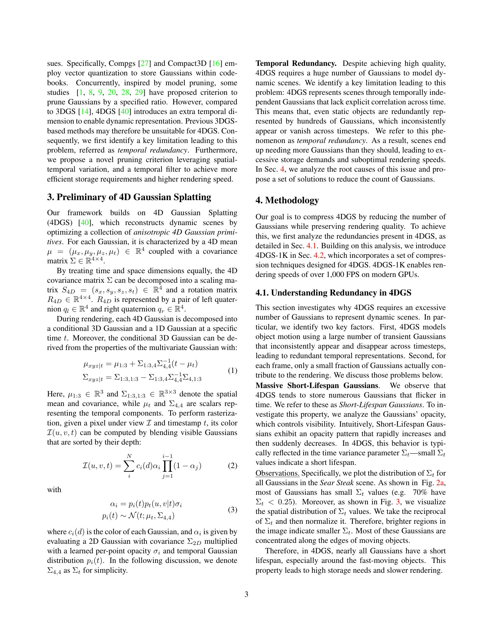
🔼 This figure provides a detailed analysis of temporal redundancy in 4D Gaussian splatting (4DGS). Panel (a) shows the distribution of the temporal variance (Σt) of Gaussians in vanilla 4DGS, highlighting a high concentration of Gaussians with short lifespans. The other lines in this panel show how the proposed 4DGS-1K method significantly reduces the number of these short-lived Gaussians. Panel (b) illustrates the active ratio of Gaussians during rendering across different time steps. It reveals that vanilla 4DGS spends a large portion of computation time processing inactive Gaussians, while 4DGS-1K significantly reduces this redundancy. Finally, panel (c) shows the Intersection over Union (IoU) between the active Gaussians in the first frame and subsequent frames. The high IoU values demonstrate a substantial overlap in active Gaussians across consecutive frames, indicating a potential for optimization.
read the caption
Figure 2: Temporal redundancy Study. (a) The ΣtsubscriptΣ𝑡\Sigma_{t}roman_Σ start_POSTSUBSCRIPT italic_t end_POSTSUBSCRIPT distribution of 4DGS. The red line shows the result of vanilla 4DGS. The other two lines represent our model has effectively reduced the number of transient Gaussians with small ΣtsubscriptΣ𝑡\Sigma_{t}roman_Σ start_POSTSUBSCRIPT italic_t end_POSTSUBSCRIPT. (b) The active ratio during rendering at different timestamps. It demonstrates that most of the computation time is spent on inactive Gaussians in vanilla 4DGS. However, 4DGS-1K can significantly reduce the occurrence of inactive Gaussians during rendering to avoid unnecessary computations. (c) This figure shows the IoU between the set of active Gaussians in the first frame and frame t. It proves that active Gaussians tend to overlap significantly across adjacent frames.

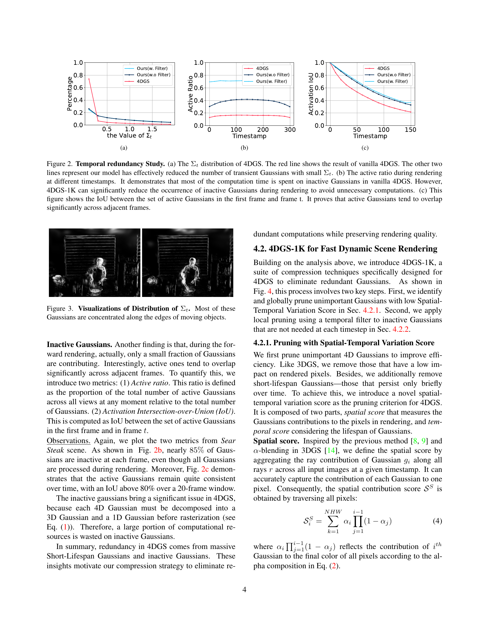
🔼 Figure 3 visualizes the distribution of the temporal variance (Σt) of 4D Gaussians in a dynamic scene. The visualization highlights that a significant portion of these Gaussians, represented by brighter areas in the image, are concentrated along the boundaries of moving objects. This observation supports the paper’s argument that a considerable number of 4D Gaussians in the 4D Gaussian Splatting (4DGS) method have short lifespans, contributing to redundancy and inefficiencies. The figure thus provides visual evidence for the temporal redundancy problem addressed by the authors.
read the caption
Figure 3: Visualizations of Distribution of ΣtsubscriptΣ𝑡\Sigma_{t}roman_Σ start_POSTSUBSCRIPT italic_t end_POSTSUBSCRIPT. Most of these Gaussians are concentrated along the edges of moving objects.

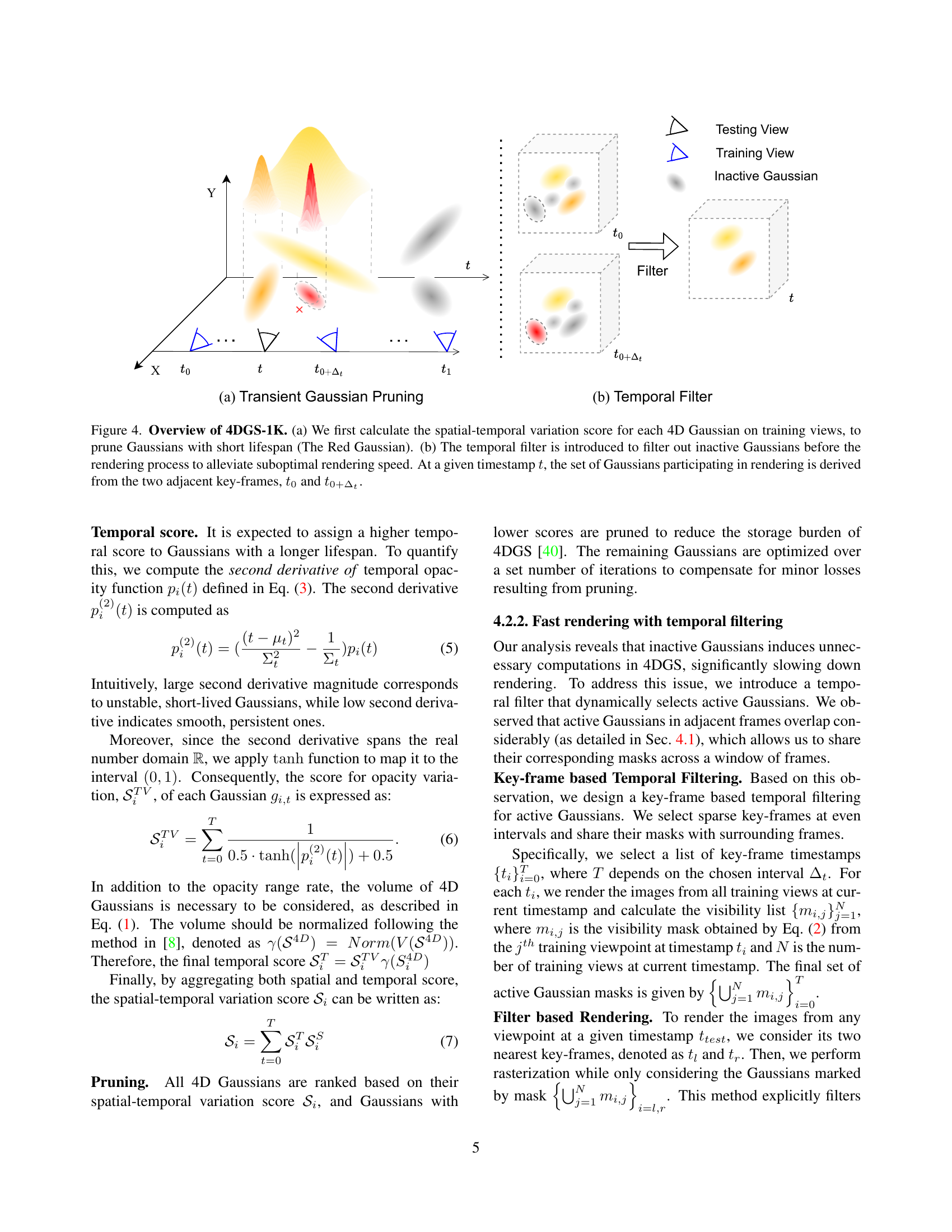
🔼 Figure 4 illustrates the two-step pruning strategy used in 4DGS-1K to improve efficiency. (a) shows the pruning of Gaussians with short lifespans using the spatial-temporal variation score. A score is calculated for each Gaussian, and those with low scores (indicating minimal impact) are removed. This step reduces redundancy caused by many Gaussians having short temporal spans. (b) shows how a temporal filter is used to remove inactive Gaussians before rendering. A mask is created to identify active Gaussians in two adjacent keyframes (t0 and t0 + Δt). Gaussians not present in this mask are excluded from the rendering process at timestamp t, thereby reducing computation time. Overall, the figure explains how 4DGS-1K reduces both storage requirements and rendering time through intelligent Gaussian pruning.
read the caption
Figure 4: Overview of 4DGS-1K. (a) We first calculate the spatial-temporal variation score for each 4D Gaussian on training views, to prune Gaussians with short lifespan (The Red Gaussian). (b) The temporal filter is introduced to filter out inactive Gaussians before the rendering process to alleviate suboptimal rendering speed. At a given timestamp t𝑡titalic_t, the set of Gaussians participating in rendering is derived from the two adjacent key-frames, t0subscript𝑡0t_{0}italic_t start_POSTSUBSCRIPT 0 end_POSTSUBSCRIPT and t0+Δtsubscript𝑡0subscriptΔ𝑡t_{0+\Delta_{t}}italic_t start_POSTSUBSCRIPT 0 + roman_Δ start_POSTSUBSCRIPT italic_t end_POSTSUBSCRIPT end_POSTSUBSCRIPT.

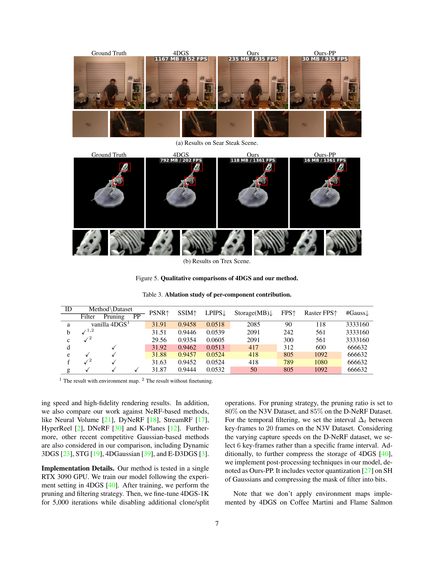
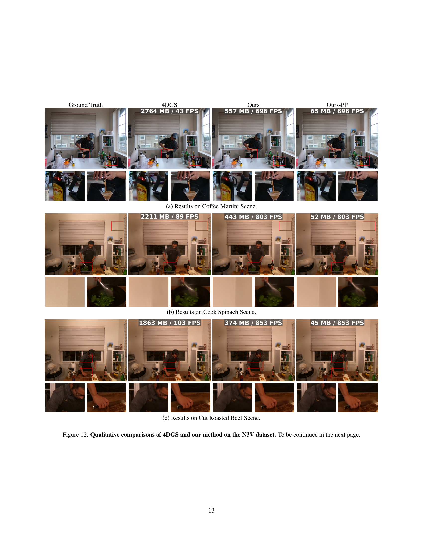
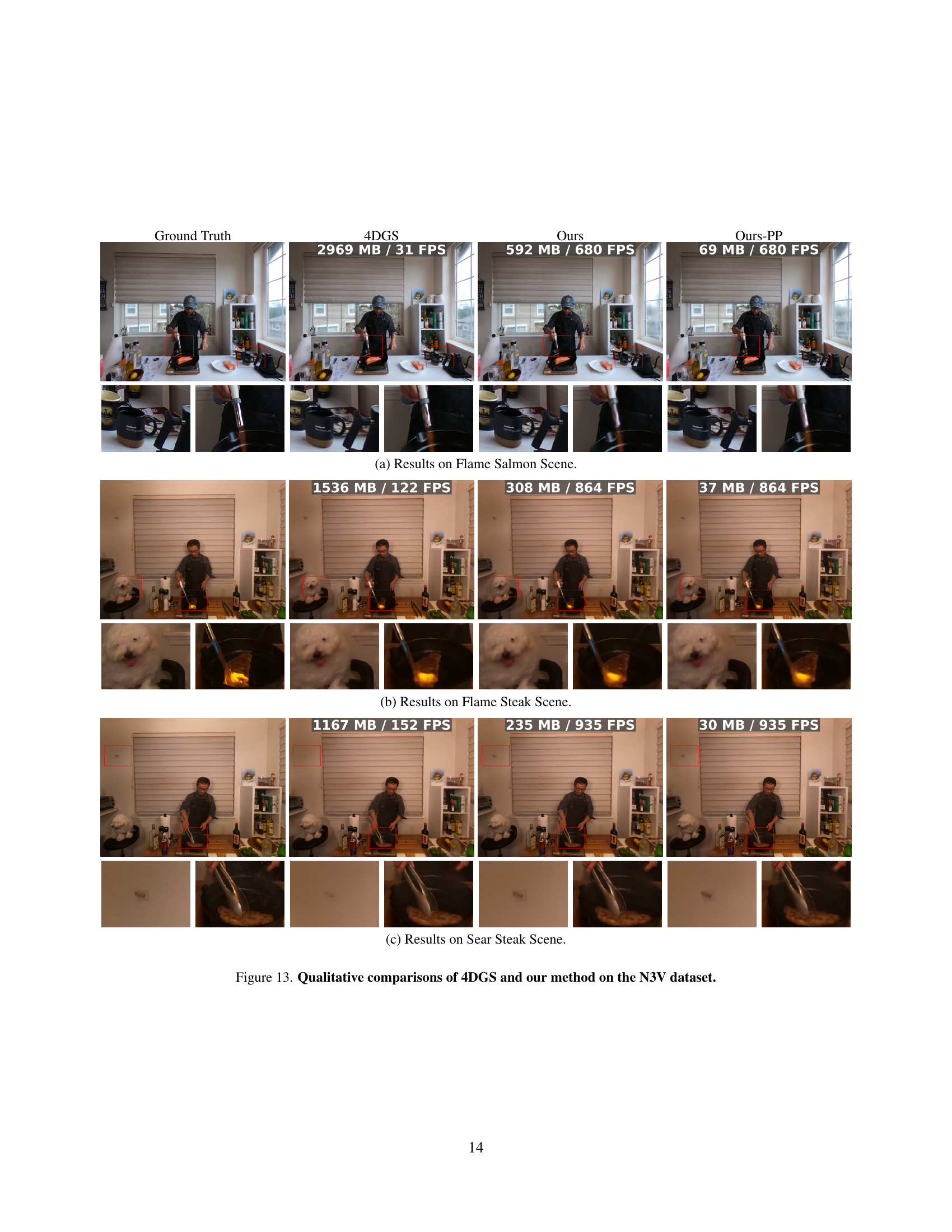
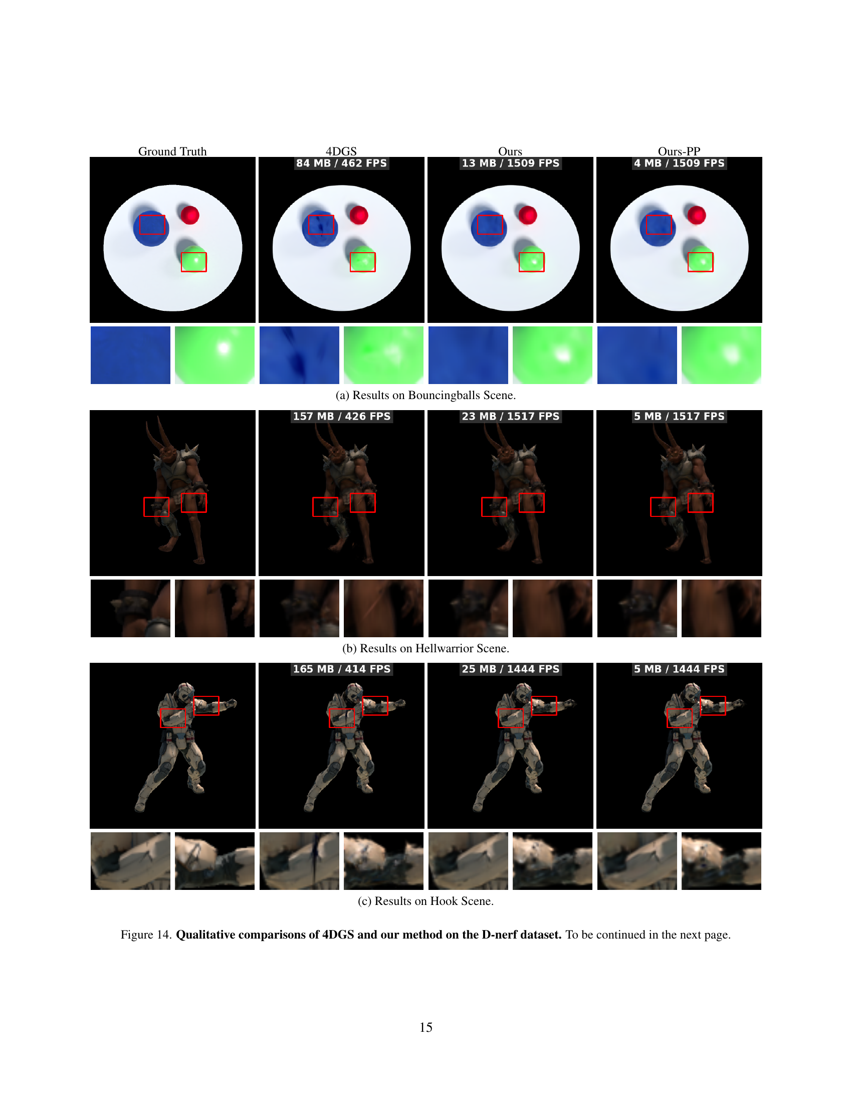
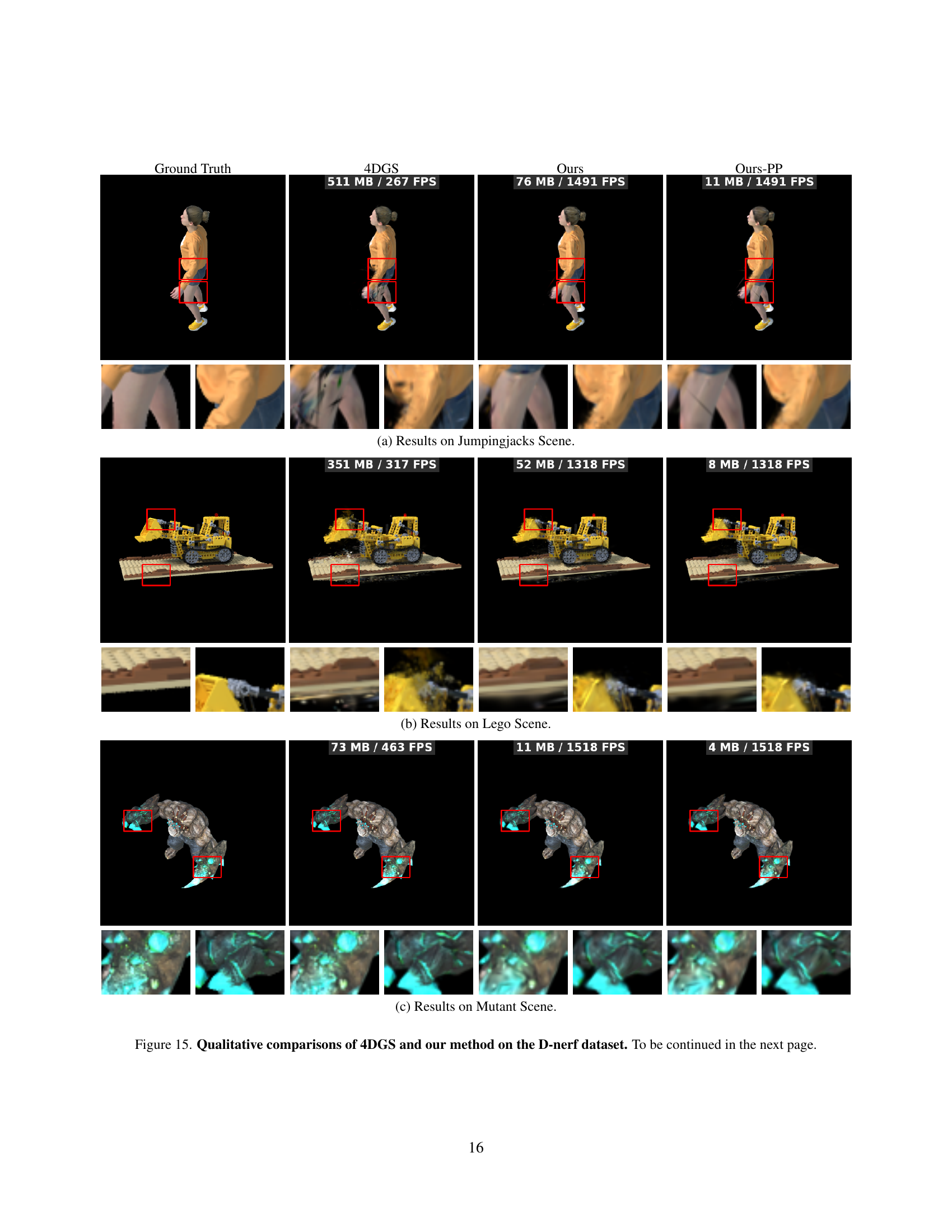
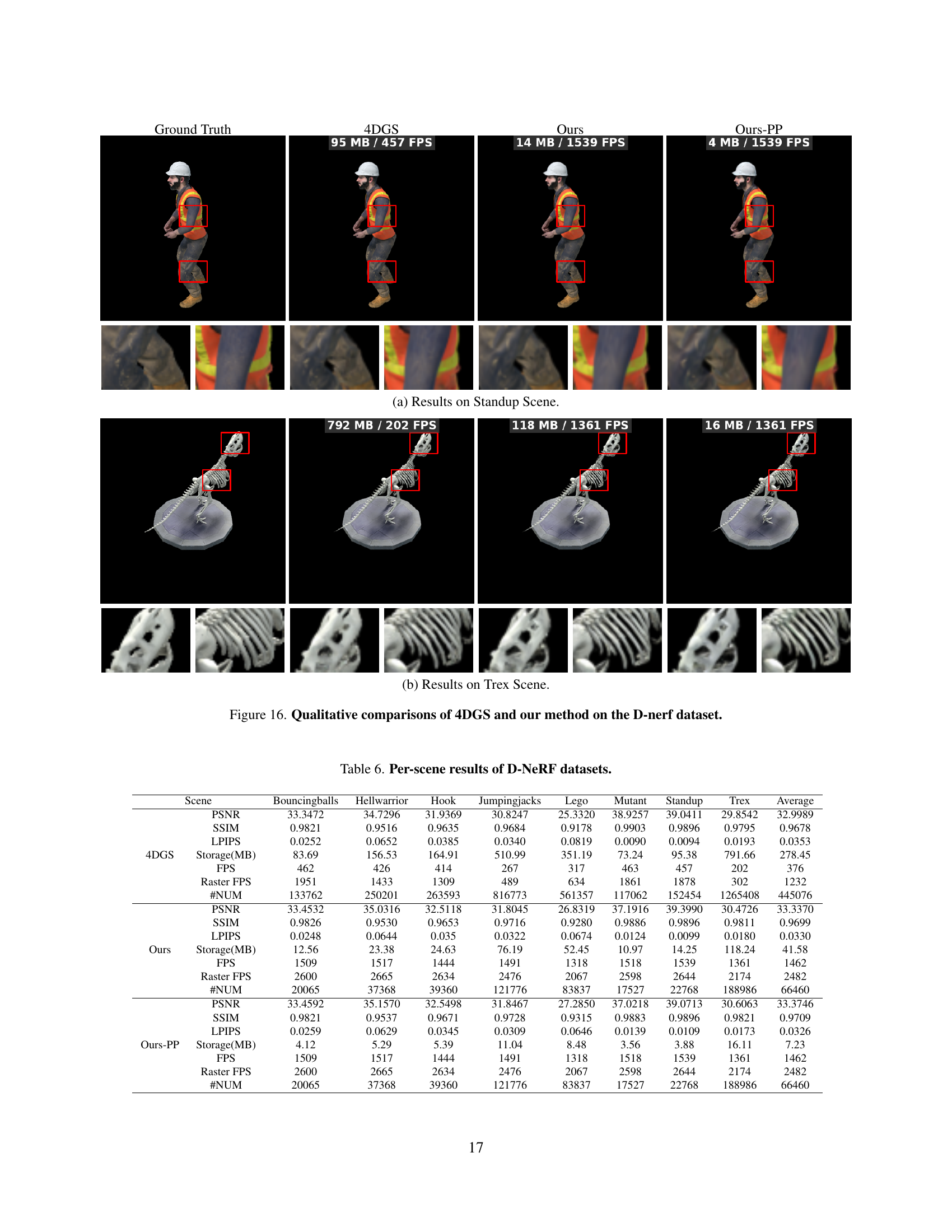
🔼 This figure presents a qualitative comparison of the results obtained using the original 4D Gaussian Splatting (4DGS) method and the proposed 4DGS-1K method. It shows visual results for two dynamic scenes (‘Sear Steak’ and ‘Trex’), comparing ground truth images with those rendered by 4DGS and the two versions of the 4DGS-1K method (one with post-processing and one without). The comparison highlights the visual similarity between 4DGS-1K’s output and the ground truth, while also demonstrating the significant reduction in storage size and increase in rendering speed achieved by the proposed method.
read the caption
Figure 5: Qualitative comparisons of 4DGS and our method.

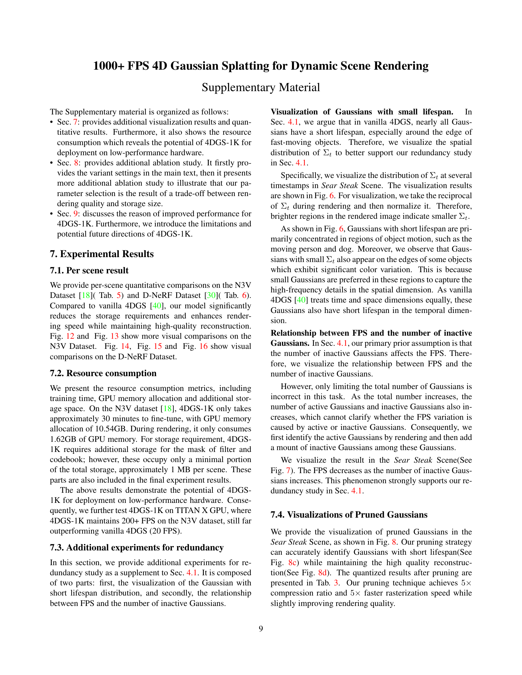
🔼 This figure visualizes the distribution of the temporal variance parameter (Σt) across all Gaussians in the Sear Steak scene. The reciprocal of Σt is taken and then normalized, resulting in brighter regions representing smaller Σt values (indicating a short lifespan for those Gaussians). The visualization shows the spatial distribution of Σt across different timestamps, highlighting where Gaussians with short lifespans are concentrated (primarily along edges of moving objects). This illustrates the temporal redundancy issue in 4DGS, where a large number of Gaussians have short lifespans.
read the caption
Figure 6: Visualizations of Distribution of ΣtsubscriptΣ𝑡\Sigma_{t}roman_Σ start_POSTSUBSCRIPT italic_t end_POSTSUBSCRIPT.

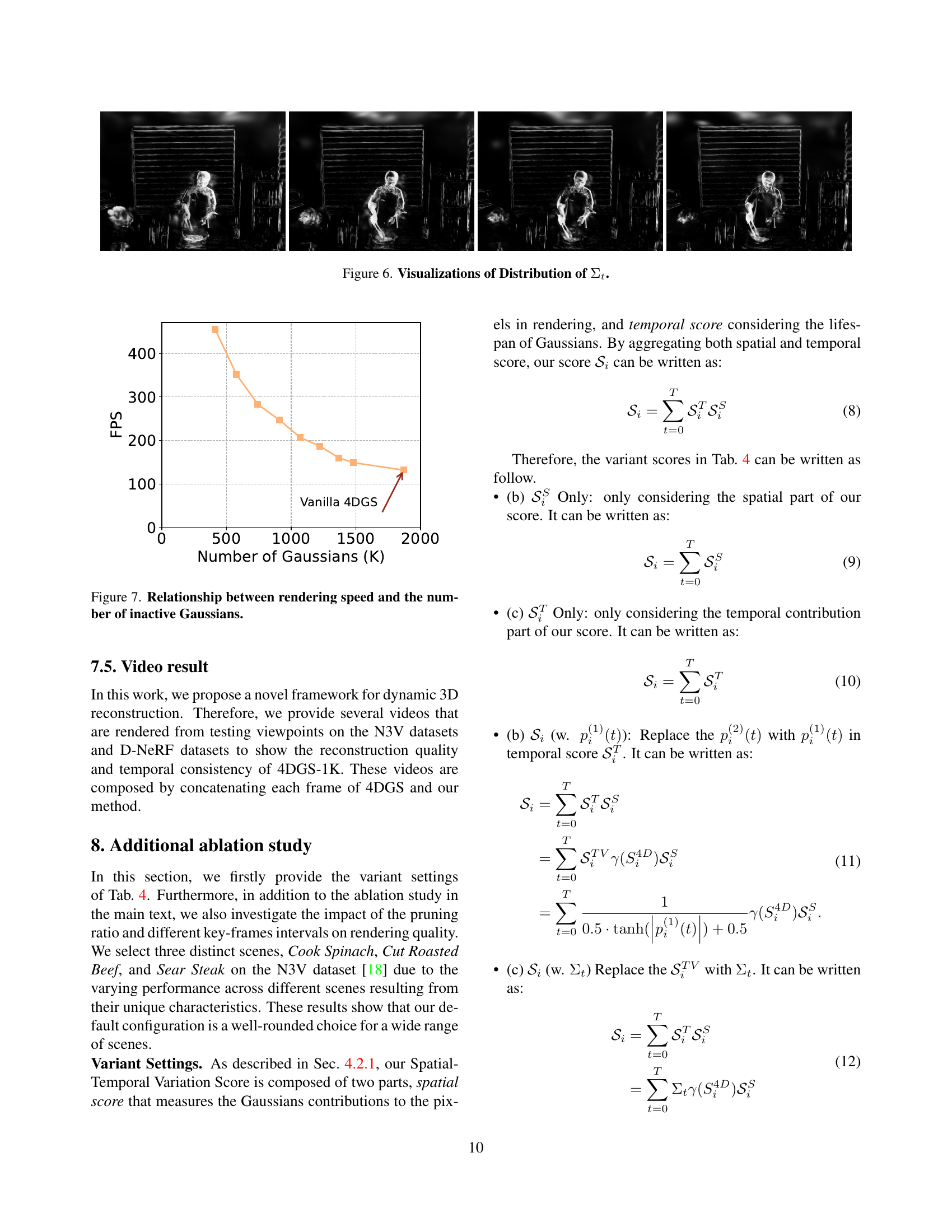
🔼 This figure demonstrates the inverse relationship between rendering speed (FPS) and the number of inactive Gaussians in a dynamic scene. As the number of inactive Gaussians increases, the rendering speed decreases. This is because the computational resources are being wasted on processing Gaussians that do not contribute to the rendered image.
read the caption
Figure 7: Relationship between rendering speed and the number of inactive Gaussians.

🔼 This figure shows a qualitative comparison of the results obtained by the proposed method (4DGS-1K) and the baseline method (4DGS) on the Sear Steak scene. The top row displays the ground truth frames of the scene. The subsequent rows show the corresponding frames rendered using vanilla 4DGS, 4DGS-1K, and 4DGS-1K with post-processing (Ours-PP). This visualization allows for a direct comparison of the visual quality and fidelity of the different methods, highlighting the improvements achieved by 4DGS-1K in terms of visual quality and compression.
read the caption
(a) Ground Truth

🔼 This figure visualizes the distribution of the temporal variance parameter (Σt) across all Gaussians in the Sear Steak scene from the Neural 3D Video dataset. The visualization uses a colormap where brighter regions indicate smaller Σt values, thus highlighting Gaussians with shorter lifespans. The plot shows that a significant portion of Gaussians in the scene exhibit short lifespans, particularly concentrated along the edges of moving objects. This observation supports the claim that 4D Gaussian Splatting often uses many short-lived Gaussians, leading to storage redundancy and slow rendering.
read the caption
(b) Distribution of ΣtsubscriptΣ𝑡\Sigma_{t}roman_Σ start_POSTSUBSCRIPT italic_t end_POSTSUBSCRIPT
🔼 This figure visualizes the effect of applying the spatial-temporal variation score pruning strategy. It shows a comparison between the original Gaussians (before pruning) and the remaining Gaussians after the pruning step in 4DGS-1K. The result demonstrates the effectiveness of the proposed method to eliminate redundant Gaussians, leading to a more compact scene representation.
read the caption
(c) Pruned Gaussians

🔼 This figure shows the result of the proposed method (4DGS-1K) on a dynamic scene. It demonstrates that the method achieves high-quality reconstruction and high rendering speed, comparable to the ground truth but using significantly less storage space than existing methods like vanilla 4DGS.
read the caption
(d) Ours

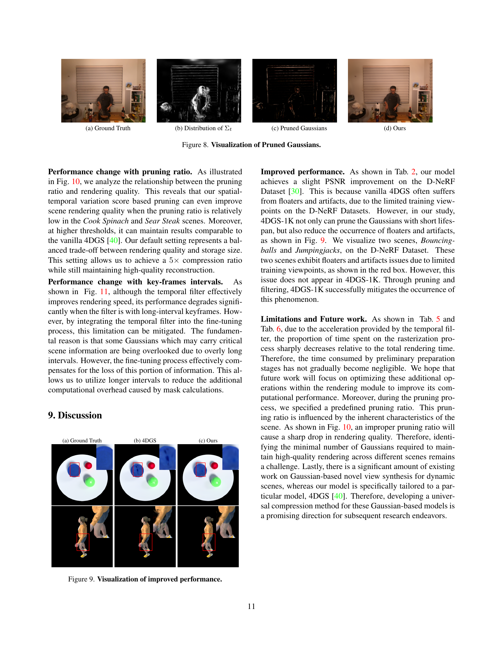
🔼 This figure visualizes the effect of the proposed pruning strategy on Gaussians. It shows four sets of images: ground truth, vanilla 4DGS, the results after pruning Gaussians using the spatial-temporal variation score, and the final results after applying the temporal filter. The comparison highlights how the pruning technique effectively removes redundant Gaussians while maintaining high-quality scene reconstruction. The reduction in the number of Gaussians leads to significant improvements in both storage and rendering speed.
read the caption
Figure 8: Visualization of Pruned Gaussians.
More on tables
| Method | PSNR | SSIM | LPIPS | Storage(MB) | FPS | Raster FPS | #Gauss |
| DNeRF[30] | 29.67 | 0.95 | 0.08 | - | 0.1 | - | - |
| TiNeuVox[10] | 32.67 | 0.97 | 0.04 | - | 1.6 | - | - |
| K-Planes[12] | 31.07 | 0.97 | 0.02 | - | 1.2 | - | - |
| 4DGaussian[39] | 32.99 | 0.97 | 0.05 | 18 | 104 | - | - |
| Deformable3DGS[41] | 40.43 | 0.99 | 0.01 | 27 | 70 | - | 131428 |
| 4D-RotorGS[7] | 34.26 | 0.97 | 0.03 | 112 | 1257 | - | - |
| 4DGS[40] | 34.09 | 0.98 | 0.02 | - | - | - | - |
| 4DGS1[40] | 32.99 | 0.97 | 0.03 | 278 | 376 | 1232 | 445076 |
| Ours | 33.34 | 0.97 | 0.03 | 42 | 1462 | 2482 | 66460 |
| Ours-PP | 33.37 | 0.97 | 0.03 | 7 | 1462 | 2482 | 66460 |
🔼 This table presents a quantitative comparison of different methods for novel view synthesis on the D-NeRF dataset. Metrics include Peak Signal-to-Noise Ratio (PSNR), Structural Similarity Index Measure (SSIM), Learned Perceptual Image Patch Similarity (LPIPS), storage size in MB, rendering FPS (frames per second), and the number of Gaussians used in the model. It allows for a comparison of the performance and efficiency of various techniques in representing and rendering dynamic scenes.
read the caption
Table 2: Quantitative comparisons on the D-NeRF Dataset.
| ID | Method\Dataset | PSNR | SSIM | LPIPS | Storage(MB) | FPS | Raster FPS | #Gauss | ||
| Filter | Pruning | PP | ||||||||
| a | vanilla 4DGS1 | 31.91 | 0.9458 | 0.0518 | 2085 | 90 | 118 | 3333160 | ||
| b | ✓1,2 | 31.51 | 0.9446 | 0.0539 | 2091 | 242 | 561 | 3333160 | ||
| c | ✓2 | 29.56 | 0.9354 | 0.0605 | 2091 | 300 | 561 | 3333160 | ||
| d | ✓ | 31.92 | 0.9462 | 0.0513 | 417 | 312 | 600 | 666632 | ||
| e | ✓ | ✓ | 31.88 | 0.9457 | 0.0524 | 418 | 805 | 1092 | 666632 | |
| f | ✓2 | ✓ | 31.63 | 0.9452 | 0.0524 | 418 | 789 | 1080 | 666632 | |
| g | ✓ | ✓ | ✓ | 31.87 | 0.9444 | 0.0532 | 50 | 805 | 1092 | 666632 |
🔼 This table presents an ablation study evaluating the individual and combined contributions of different components within the proposed 4DGS-1K method. It systematically analyzes the effects of the spatial-temporal variation score (STVS) based pruning, the temporal filter, and the combination of both, on key metrics like PSNR, SSIM, LPIPS, storage size, and rendering speed (both raster and total FPS). By comparing various configurations, the study quantifies the impact of each component and validates the effectiveness of the proposed approach.
read the caption
Table 3: Ablation study of per-component contribution.
| ID | Model | Sear Steak | Flame Salmon |
| a | 4DGS w/o Prune | 33.60 | 29.10 |
| b | Only | 33.62 | 28.75 |
| c | Only | 33.59 | 28.79 |
| d | (w. ) | 33.67 | 28.81 |
| e | (w. ) | 33.47 | 28.71 |
| f | Ours | 33.76 | 28.90 |
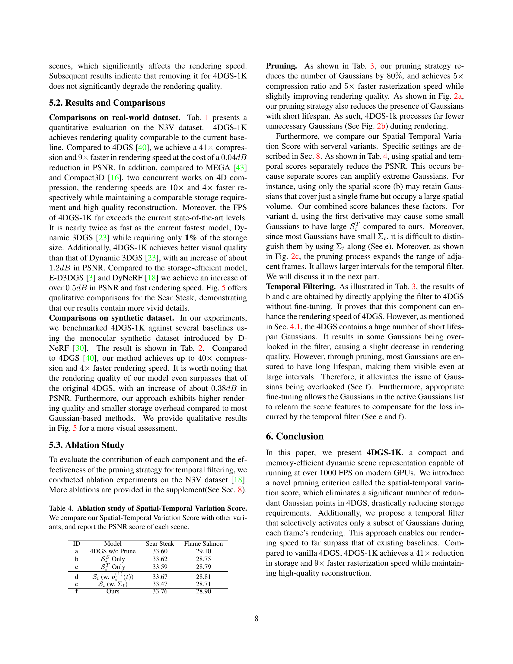
🔼 This ablation study investigates the impact of different spatial-temporal variation score components on the PSNR (Peak Signal-to-Noise Ratio) of various scenes. The study compares the full Spatial-Temporal Variation Score against versions using only the spatial component, only the temporal component, a modified temporal component using the first derivative of opacity instead of the second derivative, and a variant that uses the temporal variance parameter (Στ) instead of the temporal variation score. The PSNR values for each scene under these different scoring methods are presented, allowing for an assessment of the individual contributions of the spatial and temporal aspects of the score in achieving high PSNR values.
read the caption
Table 4: Ablation study of Spatial-Temporal Variation Score. We compare our Spatial-Temporal Variation Score with other variants, and report the PSNR score of each scene.
| Scene | Coffee Martini | Cook Spinach | Cut Roasted Beef | Flame Salmon | Flame Steak | Sear Steak | Average | |
| 4DGS | PSNR | 27.9286 | 33.1651 | 33.8849 | 29.1009 | 33.7970 | 33.6031 | 31.9133 |
| SSIM | 0.9160 | 0.9545 | 0.9589 | 0.9236 | 0.9615 | 0.9607 | 0.9459 | |
| LPIPS | 0.0759 | 0.0449 | 0.0408 | 0.0691 | 0.0383 | 0.0418 | 0.0518 | |
| Storage(MB) | 2764 | 2211 | 1863 | 2969 | 1536 | 1167 | 2085 | |
| FPS | 43 | 89 | 103 | 31 | 122 | 152 | 90 | |
| Raster FPS | 75 | 103 | 122 | 70 | 148 | 195 | 118 | |
| #NUM | 4441271 | 3530165 | 2979832 | 4719443 | 2457356 | 1870891 | 3333160 | |
| Ours | PSNR | 28.5780 | 33.2613 | 33.6092 | 28.8488 | 33.2804 | 33.7150 | 31.8821 |
| SSIM | 0.9185 | 0.9553 | 0.9570 | 0.9221 | 0.9598 | 0.9615 | 0.9457 | |
| LPIPS | 0.0726 | 0.0459 | 0.0435 | 0.0707 | 0.0417 | 0.0401 | 0.0524 | |
| Storage(MB) | 557.4 | 443.11 | 374.05 | 592.4 | 308.4 | 234.8 | 418.36 | |
| FPS | 696 | 803 | 853 | 680 | 864 | 935 | 805 | |
| Raster FPS | 901 | 1088 | 1163 | 879 | 1189 | 1332 | 1092 | |
| #NUM | 888254 | 706033 | 595967 | 943889 | 491471 | 374178 | 666632 | |
| Ours-PP | PSNR | 28.5472 | 33.0641 | 33.7767 | 28.9878 | 33.2519 | 33.6053 | 31.8722 |
| SSIM | 0.9166 | 0.9540 | 0.9562 | 0.9209 | 0.9581 | 0.9604 | 0.9444 | |
| LPIPS | 0.0744 | 0.0467 | 0.0445 | 0.0712 | 0.0421 | 0.0402 | 0.0532 | |
| Storage(MB) | 64.94 | 52.04 | 44.54 | 69.24 | 36.94 | 29.34 | 49.50 | |
| FPS | 696 | 803 | 853 | 680 | 864 | 935 | 805 | |
| Raster FPS | 901 | 1088 | 1163 | 879 | 1189 | 1332 | 1092 | |
| #NUM | 888254 | 706033 | 595967 | 943889 | 491471 | 374178 | 666632 | |
🔼 This table presents a per-scene breakdown of quantitative results for the Neural 3D Video (N3V) dataset. For each of the six scenes in the dataset (Coffee Martini, Cook Spinach, Cut Roasted Beef, Flame Salmon, Flame Steak, Sear Steak), the table provides key metrics evaluating the performance of the proposed 4DGS-1K model and compares it to the original 4DGS model. The metrics include Peak Signal-to-Noise Ratio (PSNR), Structural Similarity Index Measure (SSIM), Learned Perceptual Image Patch Similarity (LPIPS), storage size in MB, frames per second (FPS), raster FPS, and the number of Gaussians used. The results offer a scene-specific comparison of rendering quality and efficiency.
read the caption
Table 5: Per-scene results of N3V datasets.
| Scene | Bouncingballs | Hellwarrior | Hook | Jumpingjacks | Lego | Mutant | Standup | Trex | Average | |
| 4DGS | PSNR | 33.3472 | 34.7296 | 31.9369 | 30.8247 | 25.3320 | 38.9257 | 39.0411 | 29.8542 | 32.9989 |
| SSIM | 0.9821 | 0.9516 | 0.9635 | 0.9684 | 0.9178 | 0.9903 | 0.9896 | 0.9795 | 0.9678 | |
| LPIPS | 0.0252 | 0.0652 | 0.0385 | 0.0340 | 0.0819 | 0.0090 | 0.0094 | 0.0193 | 0.0353 | |
| Storage(MB) | 83.69 | 156.53 | 164.91 | 510.99 | 351.19 | 73.24 | 95.38 | 791.66 | 278.45 | |
| FPS | 462 | 426 | 414 | 267 | 317 | 463 | 457 | 202 | 376 | |
| Raster FPS | 1951 | 1433 | 1309 | 489 | 634 | 1861 | 1878 | 302 | 1232 | |
| #NUM | 133762 | 250201 | 263593 | 816773 | 561357 | 117062 | 152454 | 1265408 | 445076 | |
| Ours | PSNR | 33.4532 | 35.0316 | 32.5118 | 31.8045 | 26.8319 | 37.1916 | 39.3990 | 30.4726 | 33.3370 |
| SSIM | 0.9826 | 0.9530 | 0.9653 | 0.9716 | 0.9280 | 0.9886 | 0.9896 | 0.9811 | 0.9699 | |
| LPIPS | 0.0248 | 0.0644 | 0.035 | 0.0322 | 0.0674 | 0.0124 | 0.0099 | 0.0180 | 0.0330 | |
| Storage(MB) | 12.56 | 23.38 | 24.63 | 76.19 | 52.45 | 10.97 | 14.25 | 118.24 | 41.58 | |
| FPS | 1509 | 1517 | 1444 | 1491 | 1318 | 1518 | 1539 | 1361 | 1462 | |
| Raster FPS | 2600 | 2665 | 2634 | 2476 | 2067 | 2598 | 2644 | 2174 | 2482 | |
| #NUM | 20065 | 37368 | 39360 | 121776 | 83837 | 17527 | 22768 | 188986 | 66460 | |
| Ours-PP | PSNR | 33.4592 | 35.1570 | 32.5498 | 31.8467 | 27.2850 | 37.0218 | 39.0713 | 30.6063 | 33.3746 |
| SSIM | 0.9821 | 0.9537 | 0.9671 | 0.9728 | 0.9315 | 0.9883 | 0.9896 | 0.9821 | 0.9709 | |
| LPIPS | 0.0259 | 0.0629 | 0.0345 | 0.0309 | 0.0646 | 0.0139 | 0.0109 | 0.0173 | 0.0326 | |
| Storage(MB) | 4.12 | 5.29 | 5.39 | 11.04 | 8.48 | 3.56 | 3.88 | 16.11 | 7.23 | |
| FPS | 1509 | 1517 | 1444 | 1491 | 1318 | 1518 | 1539 | 1361 | 1462 | |
| Raster FPS | 2600 | 2665 | 2634 | 2476 | 2067 | 2598 | 2644 | 2174 | 2482 | |
| #NUM | 20065 | 37368 | 39360 | 121776 | 83837 | 17527 | 22768 | 188986 | 66460 | |
🔼 This table presents a quantitative comparison of different methods on the D-NeRF dataset. For each scene in the dataset, it shows the Peak Signal-to-Noise Ratio (PSNR), Structural Similarity Index Measure (SSIM), Learned Perceptual Image Patch Similarity (LPIPS), storage in MB, frames per second (FPS), raster FPS, and the number of Gaussians used. The methods compared include the baseline 4DGS, and the proposed method (Ours and Ours-PP). This allows for a comprehensive evaluation of the performance of different approaches in terms of visual quality, efficiency, and computational cost.
read the caption
Table 6: Per-scene results of D-NeRF datasets.
Full paper#