TL;DR#
Vision encoders generate many tokens, increasing computational demands. This paper addresses whether all tokens are equally valuable, suggesting some can be discarded to reduce costs without compromising quality. Prior studies show many tokens can be redundant, noisy, or irrelevant, thus decreasing model performance. The work introduces a novel method using an autoencoder-based approach with Gumbel-Softmax sampling to identify the most informative tokens from encoder outputs.
Experiments with LLaVA-NeXT and LLaVA-OneVision models show the method reduces visual context length significantly, up to 50% for general tasks and 90% for specific tasks like OCR, with minimal performance loss. Selected features are essential, providing correct answers for most tasks analyzed, highlighting potential for adaptive and efficient multimodal pruning. It has scalability and low overhead with compromising performance.
Key Takeaways#
Why does it matter?#
This paper is important because it presents a novel task-agnostic method for reducing visual tokens in vision encoders, leading to efficient multimodal processing. It opens avenues for low-overhead inference and improved scalability in multimodal applications, which is increasingly relevant in resource-constrained environments.
Visual Insights#

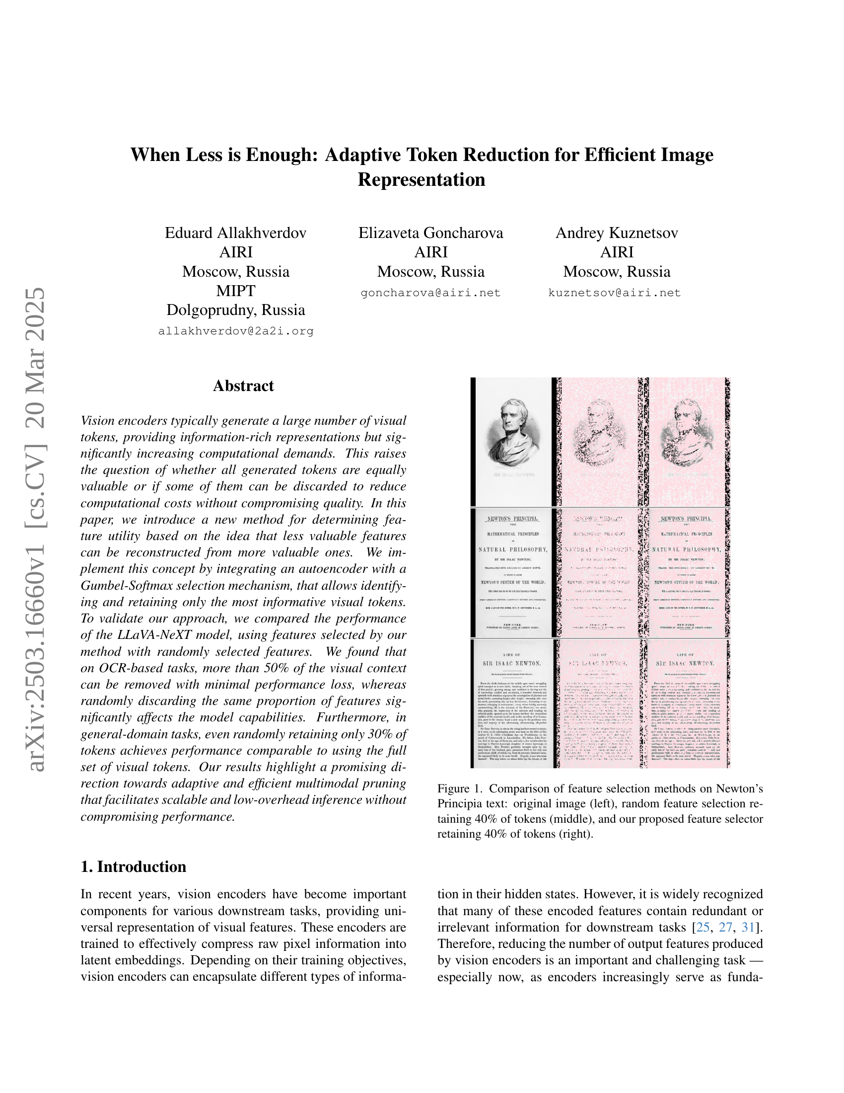
🔼 This figure compares three different approaches to feature selection applied to an image of Newton’s Principia text. The leftmost image shows the original, full-resolution image. The middle image demonstrates the result of randomly selecting and retaining only 40% of the visual tokens (features). The rightmost image shows the result of using the authors’ proposed adaptive token reduction method to select and retain 40% of the tokens. This comparison highlights the effectiveness of the proposed method in preserving important information while significantly reducing the number of features.
read the caption
Figure 1: Comparison of feature selection methods on Newton’s Principia text: original image (left), random feature selection retaining 40% of tokens (middle), and our proposed feature selector retaining 40% of tokens (right).
In-depth insights#
Token Reduction#
Token reduction techniques aim to compress visual information, addressing the computational burden of processing numerous tokens. Pruning discards irrelevant or noisy features, often guided by attention scores, while merging combines similar tokens for a compact representation. Another facet involves optimized token generation, tailoring token creation to retain essential information. Context reduction is crucial in multimodal models, where visual tokens contribute significantly to the overall input length. These methods selectively retain informative features, diminishing the computational demands, maintaining model performance, and improving the trade-off between resource usage and accuracy. Adaptive strategies are crucial to dynamically adjust the amount of retained information based on the specific task or input, optimizing performance and efficiency.
Adaptive Pruning#
Adaptive pruning in vision models offers a compelling avenue for efficiency. Instead of static compression, it dynamically adjusts based on input, retaining crucial information while discarding redundancy. This mirrors biological systems’ efficient resource allocation. Key is determining ‘informativeness’ – perhaps via gradient analysis or reconstruction error. A sophisticated strategy involves autoencoders, learning to reconstruct original features from a pruned subset, highlighting essential tokens. Gumbel-Softmax allows differentiable selection during training. Benefits extend to multimodal models by reducing visual context length, easing LLM processing. Adaptive pruning promises scalable, low-overhead inference without compromising performance, a crucial advancement for resource-constrained applications. It needs rigorous evaluation across diverse tasks and architectures to solidify its effectiveness and generalizability.
LLM Efficiency#
While not explicitly addressed with a “LLM Efficiency” section, this paper’s adaptive token reduction tackles a core challenge for efficient LLM usage in multimodal contexts. Reducing the visual token count directly lessens the computational burden on the LLM, which is crucial given LLMs’ quadratic complexity with input sequence length. The work implicitly boosts LLM efficiency by pruning redundant visual information before it reaches the LLM, allowing it to focus on the most salient features. The results, demonstrating minimal performance degradation with significant token reduction, suggests a potential path to balancing accuracy and computational cost in vision-language models. Further exploration could investigate how token selection impacts LLM’s reasoning, potentially revealing which visual features are most crucial for high-level cognitive tasks and ultimately optimize for efficient LLM processing.
Feature Selection#
Feature selection is a technique to reduce dimensionality and improve model performance. It helps to identify the most relevant features by removing redundant or irrelevant information. Effective feature selection enhances model interpretability and can prevent overfitting, leading to better generalization. Common methods include filter, wrapper, and embedded techniques, each with its own strengths and limitations in balancing computational cost and accuracy.
Gumbel-Softmax#
The Gumbel-Softmax trick, also known as the Concrete distribution, is a reparameterization technique used to sample from categorical distributions in a differentiable manner. This is crucial in scenarios where discrete sampling prevents gradient-based learning. The core idea involves adding Gumbel noise to the logits before applying the softmax function, allowing for a continuous approximation of the categorical sampling process. The temperature parameter controls the sharpness of the approximation; a lower temperature leads to a closer approximation but can increase variance in the gradients. It is often employed in variational autoencoders (VAEs) and reinforcement learning (RL) to handle discrete latent variables or action spaces. The key benefit is enabling end-to-end training by allowing gradients to flow through the sampling operation. However, careful tuning of the temperature parameter is essential to balance approximation accuracy and gradient stability, ensuring effective learning.
More visual insights#
More on figures
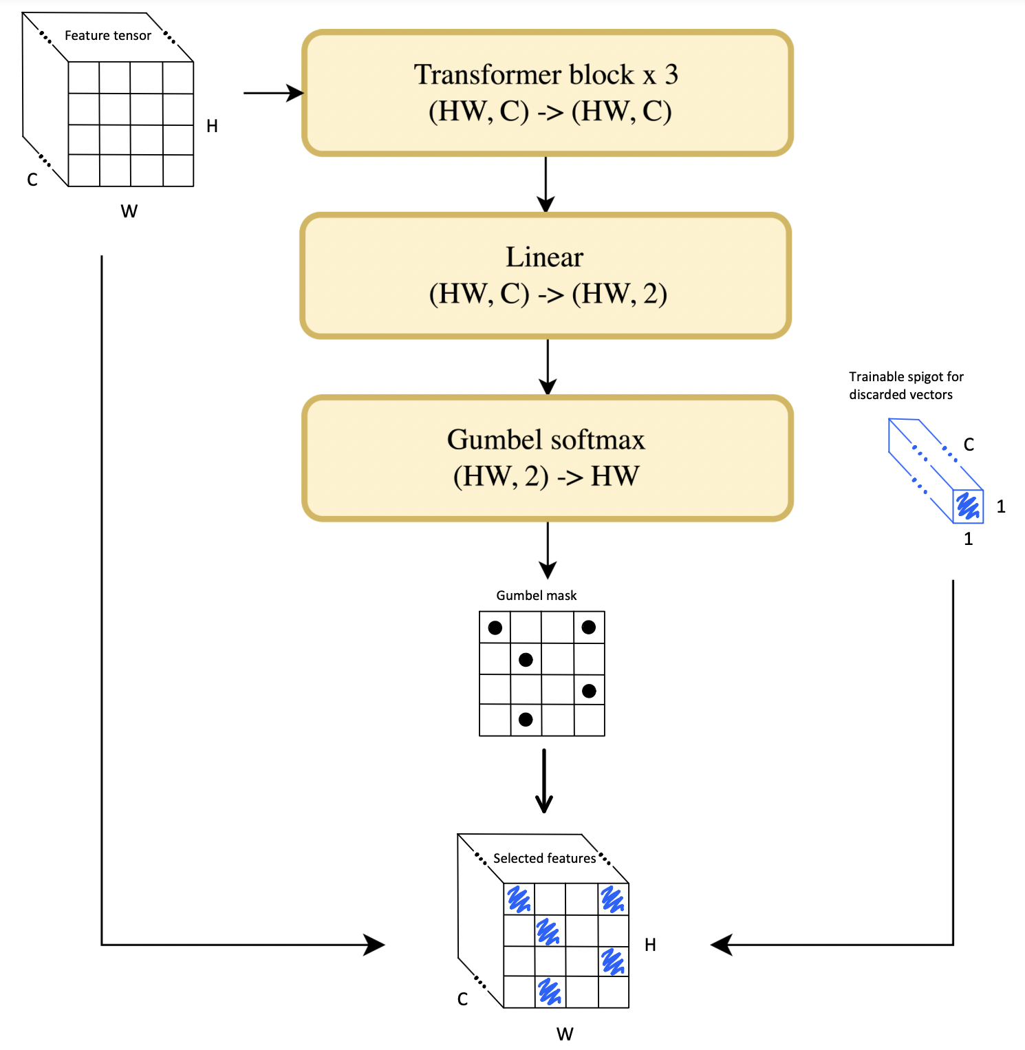
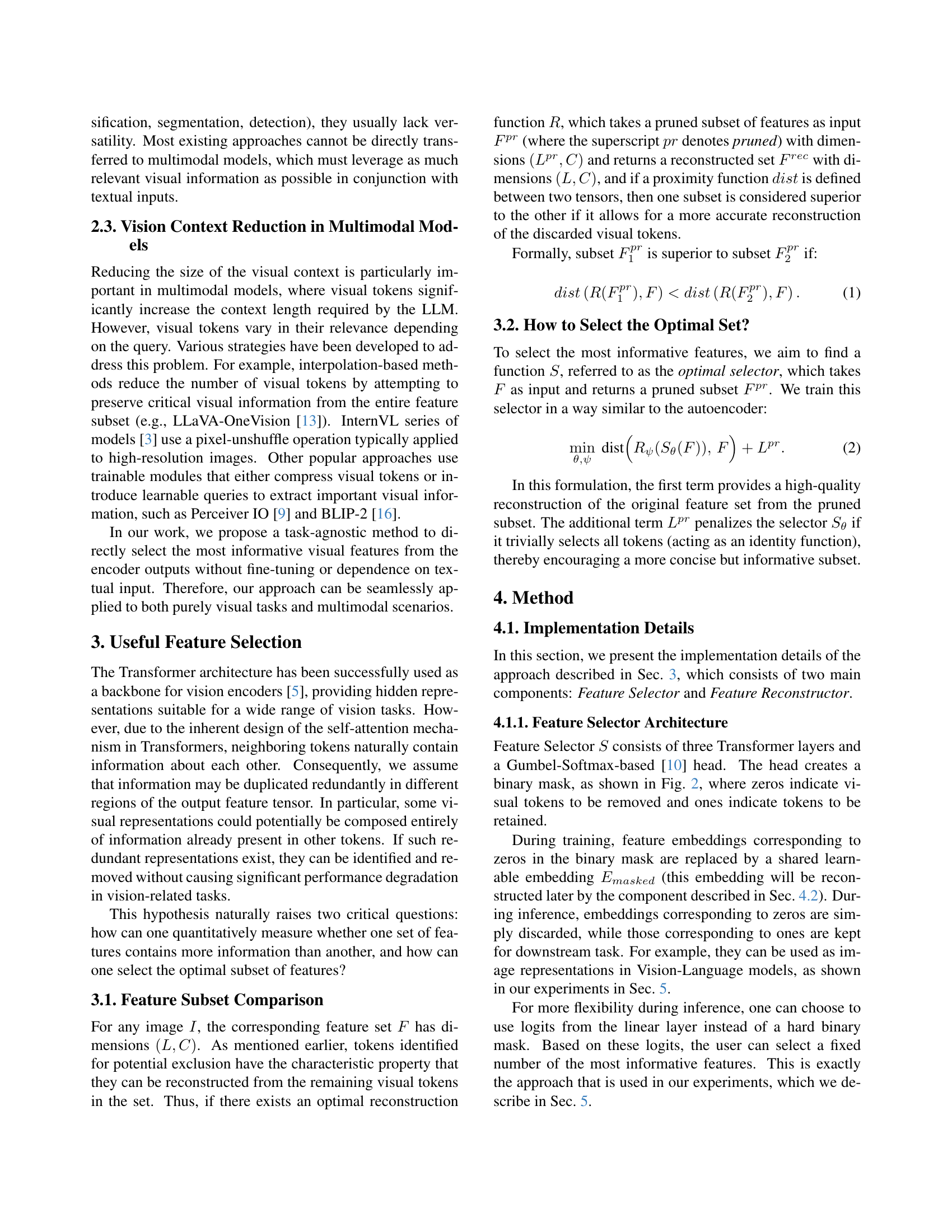
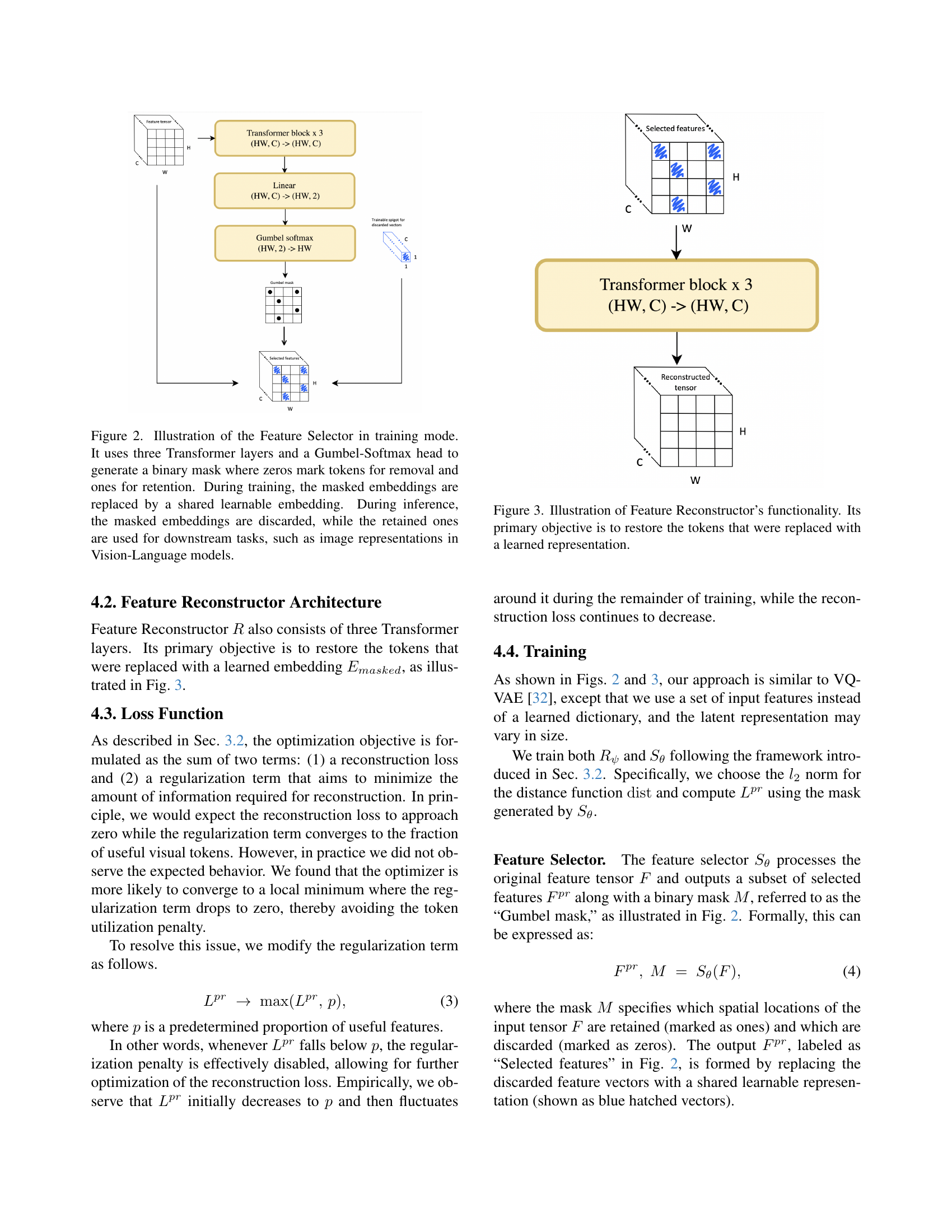
🔼 The Feature Selector, a key component of the proposed model, is illustrated. It consists of three transformer layers followed by a Gumbel-Softmax head. This head generates a binary mask to identify tokens to keep (marked as ‘1’) or discard (marked as ‘0’). During training, the discarded tokens are replaced with a shared learnable embedding. Importantly, during inference, these discarded tokens are simply removed, leading to a more efficient representation. The retained tokens are then used for downstream tasks.
read the caption
Figure 2: Illustration of the Feature Selector in training mode. It uses three Transformer layers and a Gumbel-Softmax head to generate a binary mask where zeros mark tokens for removal and ones for retention. During training, the masked embeddings are replaced by a shared learnable embedding. During inference, the masked embeddings are discarded, while the retained ones are used for downstream tasks, such as image representations in Vision-Language models.

🔼 The Feature Reconstructor is a crucial part of the proposed feature selection method. It’s a three-layer Transformer network designed to reconstruct the visual tokens that were masked (set to zero) by the Feature Selector. These masked tokens were temporarily replaced during training with a learned, shared representation. The Reconstructor’s job is to take the pruned set of features (those not masked) and generate a reconstruction of the complete feature set, attempting to recover the information lost during the pruning process. The effectiveness of this reconstruction is a key factor in evaluating which tokens are truly essential and which can be discarded without significant performance loss.
read the caption
Figure 3: Illustration of Feature Reconstructor’s functionality. Its primary objective is to restore the tokens that were replaced with a learned representation.

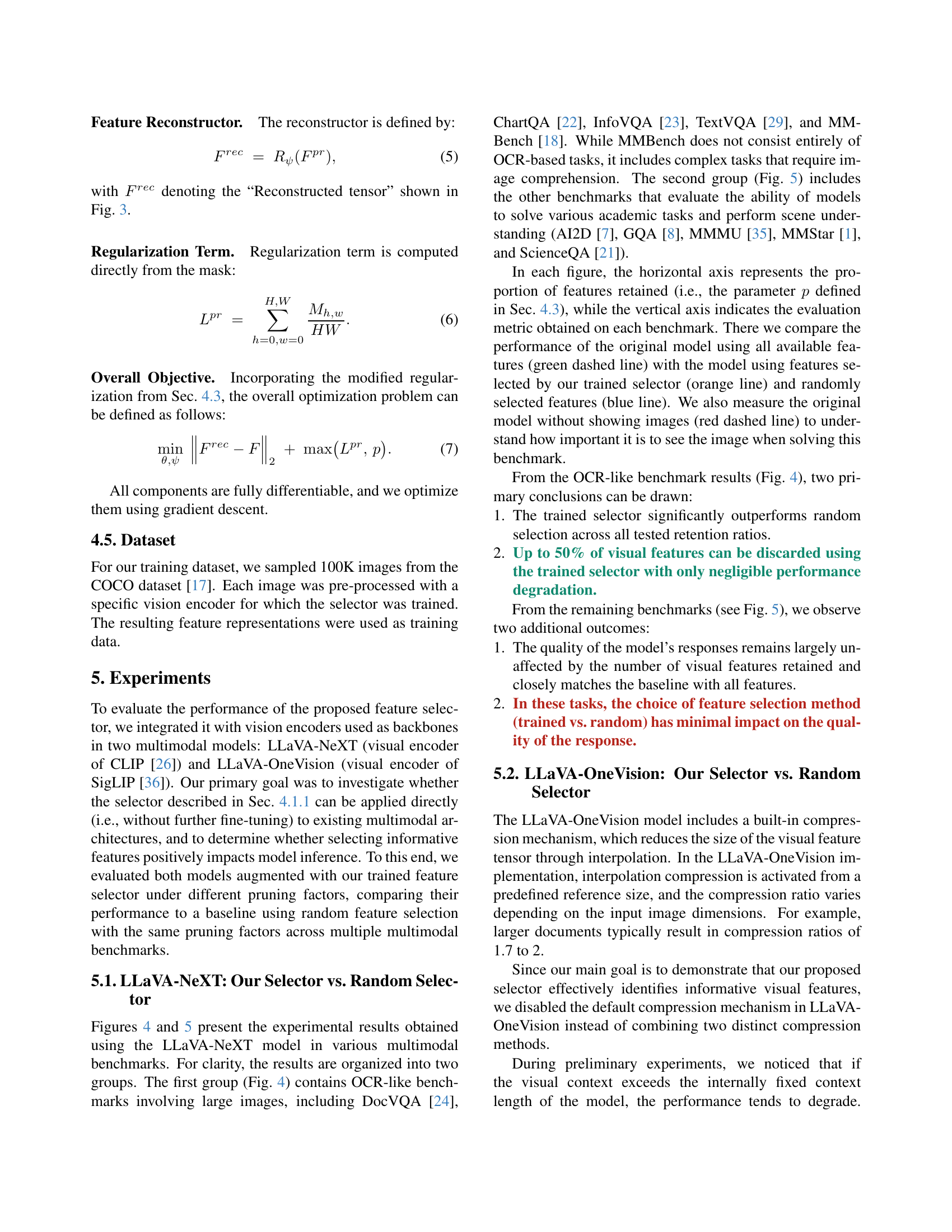
🔼 This figure displays a comparison of the LLaVA-NeXT model’s performance across various text-based benchmarks using three different feature selection methods: the proposed selector, a random selector, and no feature selection (using all features). The x-axis represents the percentage of features retained, while the y-axis shows the performance metric (likely accuracy or a similar measure) for each benchmark. The performance of the model without any image input is also shown as a baseline. This allows for an evaluation of the effectiveness of the proposed feature selection technique in maintaining performance while reducing computational cost.
read the caption
Figure 4: Comparison of LLaVA-NeXT performance with our selector (orange) and random selector (blue) on text-based benchmarks. The green dashed line represents the baseline performance using all features. The red dashed line represents the model’s performance without image input.

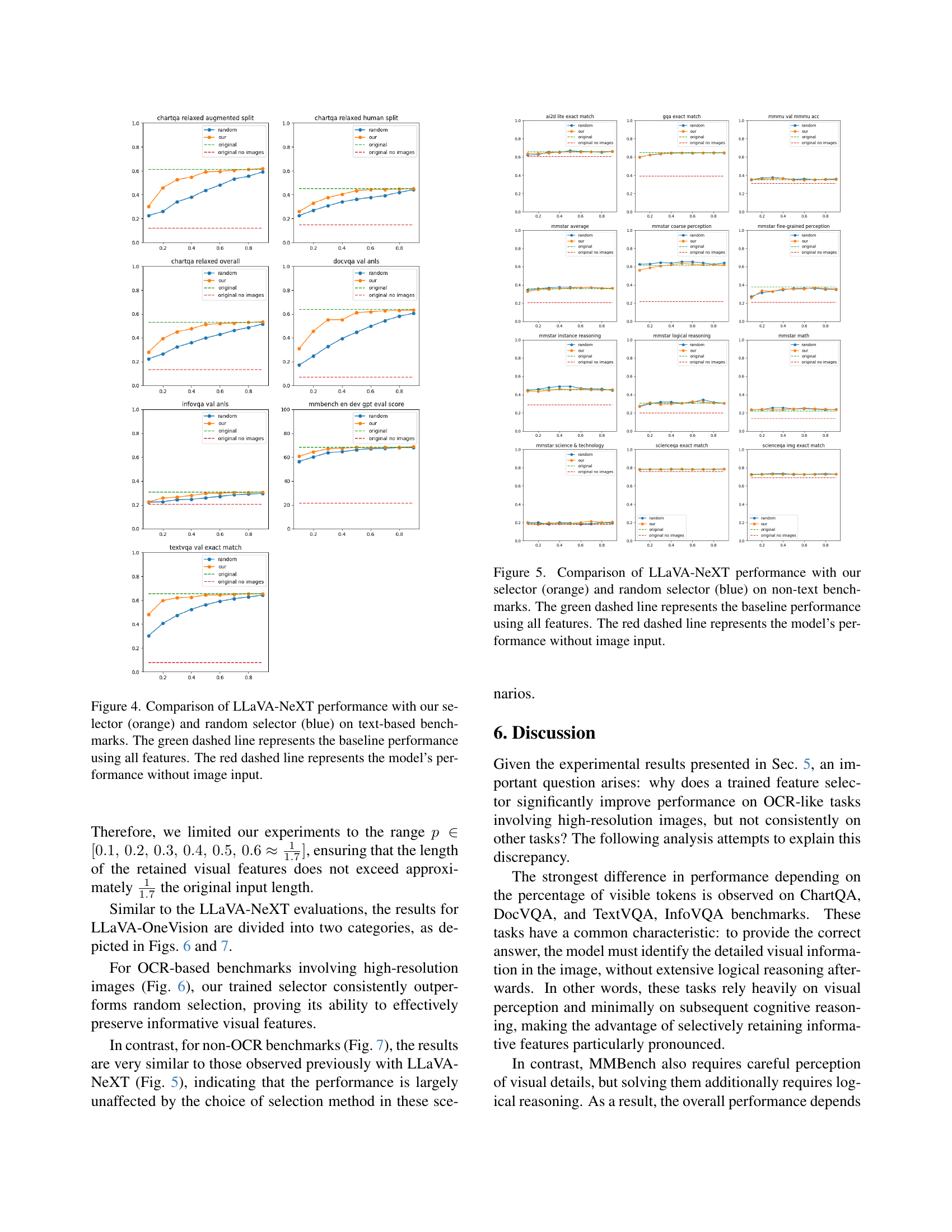
🔼 This figure compares the performance of the LLaVA-NeXT model on several non-text based benchmarks when using different feature selection methods. The performance is shown for three scenarios: using all features (green dashed line), using features selected by the proposed method (orange line), and using randomly selected features (blue line). A fourth line (red dashed line) shows the model’s performance without any visual input, providing a baseline for assessing the impact of visual information. The x-axis represents the percentage of features retained, and the y-axis represents the performance metric. This allows for a comparison of the effectiveness of the proposed approach versus random feature selection across multiple benchmarks at different levels of feature reduction.
read the caption
Figure 5: Comparison of LLaVA-NeXT performance with our selector (orange) and random selector (blue) on non-text benchmarks. The green dashed line represents the baseline performance using all features. The red dashed line represents the model’s performance without image input.

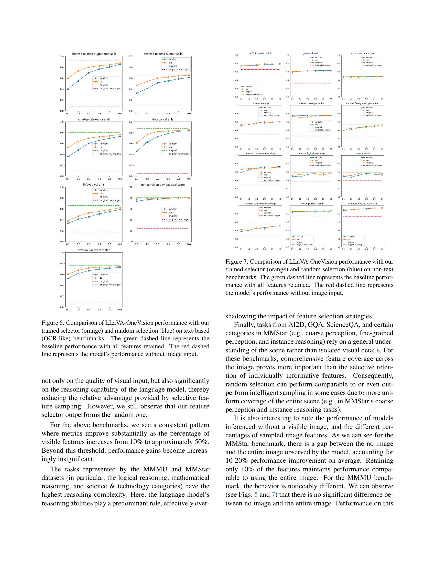
🔼 This figure compares the performance of the LLaVA-OneVision model on text-based (OCR-like) benchmarks using three different feature selection methods: our trained feature selector, random feature selection, and using all features. The x-axis shows the percentage of features retained, while the y-axis displays the performance metric (likely accuracy). The orange line represents our trained selector, the blue line represents random selection, the green dashed line shows the baseline performance using all features, and the red dashed line demonstrates the model’s performance without any image input. This visualization helps to understand how effective our feature selection is in maintaining or improving model performance while reducing the number of features required, especially compared to random selection.
read the caption
Figure 6: Comparison of LLaVA-OneVision performance with our trained selector (orange) and random selection (blue) on text-based (OCR-like) benchmarks. The green dashed line represents the baseline performance with all features retained. The red dashed line represents the model’s performance without image input.

🔼 Figure 7 displays a comparison of the LLaVA-OneVision model’s performance using different feature selection methods on non-text-based benchmarks. The model’s performance is evaluated when using all available features (baseline), features selected by the proposed trained selector, and randomly selected features. The results highlight how the proposed method compares to random selection across various metrics, showcasing its effectiveness in preserving performance even with reduced feature sets. A control is included to show the model’s performance without any image input.
read the caption
Figure 7: Comparison of LLaVA-OneVision performance with our trained selector (orange) and random selection (blue) on non-text benchmarks. The green dashed line represents the baseline performance with all features retained. The red dashed line represents the model’s performance without image input.
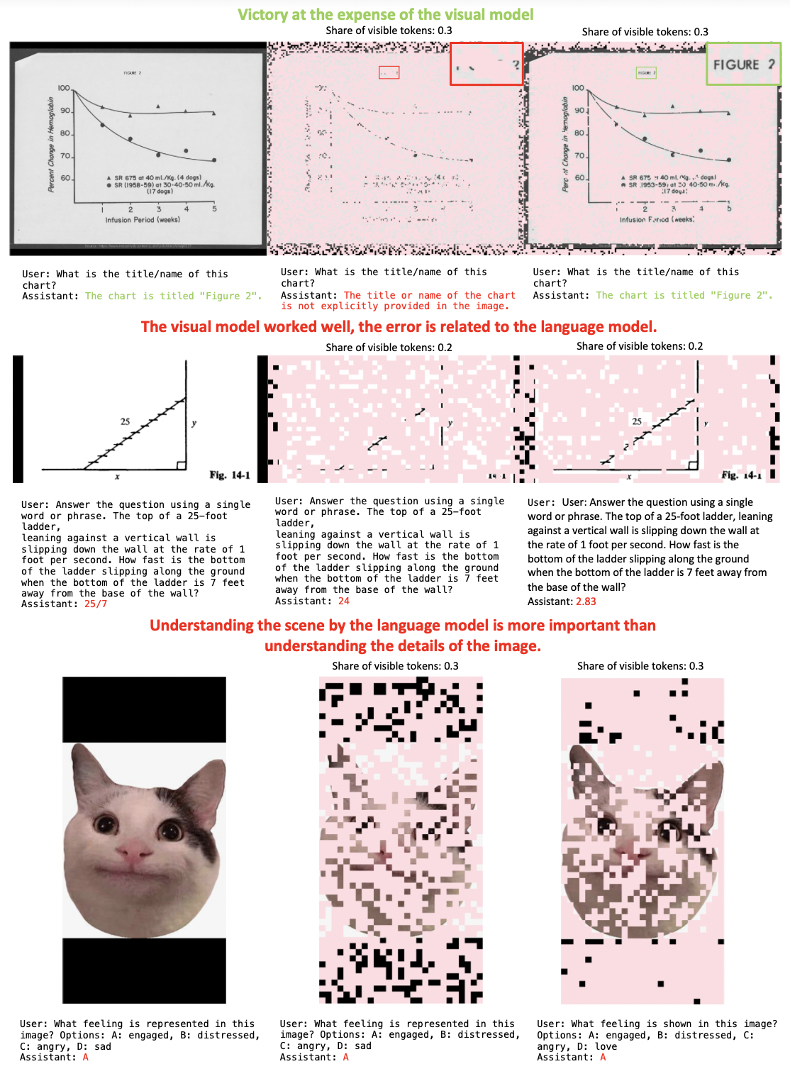
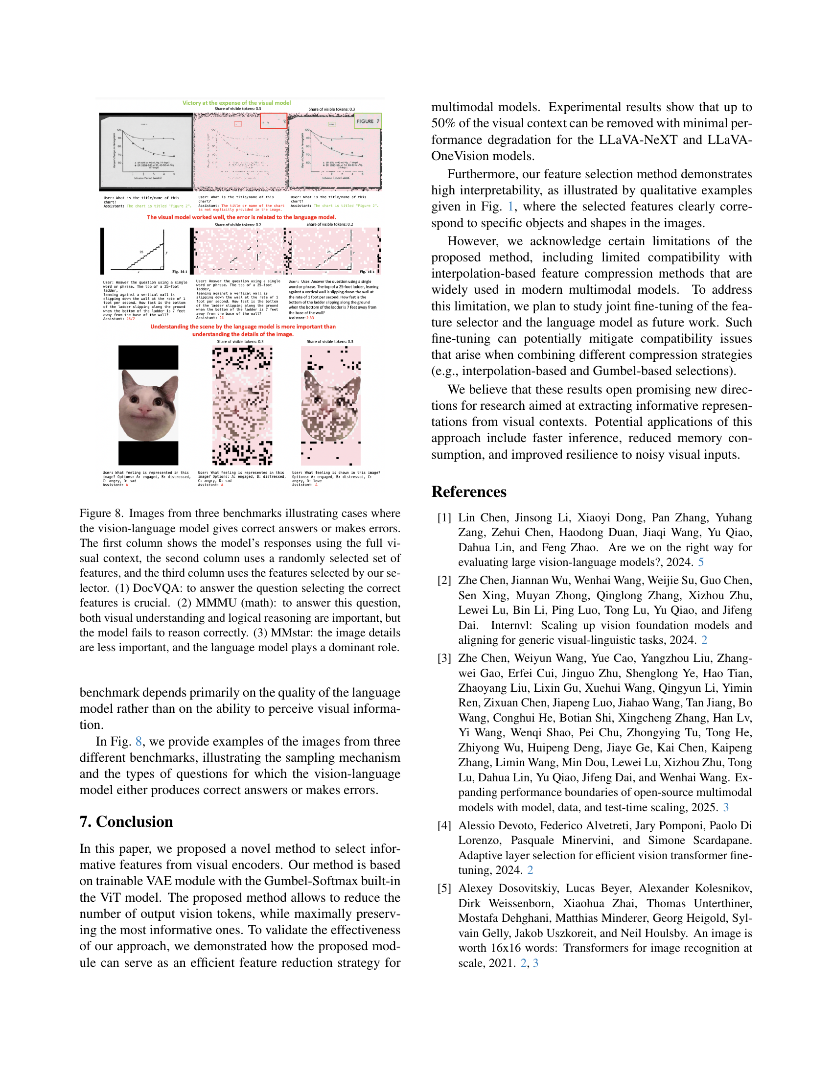
🔼 Figure 8 demonstrates the performance of the vision-language model with different feature selection methods on three benchmark datasets: DocVQA, MMMU, and MMStar. Each row shows an example image from a different benchmark. The first column shows the model’s response using all visual features, while the second uses randomly selected features and the third uses features selected by the proposed method. DocVQA showcases a scenario where selecting the correct features is essential for accurate responses. MMMU presents a task where both visual understanding and reasoning are crucial but the model struggles to reason correctly. In the MMStar example, the image details are less critical than the language model’s reasoning capacity, highlighting the importance of language processing in some tasks. This figure effectively illustrates how the importance of image features varies across different task types.
read the caption
Figure 8: Images from three benchmarks illustrating cases where the vision-language model gives correct answers or makes errors. The first column shows the model’s responses using the full visual context, the second column uses a randomly selected set of features, and the third column uses the features selected by our selector. (1) DocVQA: to answer the question selecting the correct features is crucial. (2) MMMU (math): to answer this question, both visual understanding and logical reasoning are important, but the model fails to reason correctly. (3) MMstar: the image details are less important, and the language model plays a dominant role.
Full paper#