TL;DR#
3D Gaussian Splatting (3DGS) is a powerful technique for real-time rendering, but it requires significant storage and memory. Recent studies use fewer Gaussians with high-precision attributes, but existing compression methods still rely on many Gaussians. A smaller set of Gaussians becomes sensitive to lossy compression, leading to quality issues. Therefore, reducing the number of Gaussians is crucial as it directly affects computational costs.
The paper introduces Optimized Minimal Gaussians representation (OMG), which reduces storage using minimal primitives. OMG determines distinct Gaussians from near ones, minimizing redundancy and preserving quality. It introduces a compact attribute representation, capturing continuity and irregularity. A sub-vector quantization technique enhances irregularity representation while maintaining fast training. OMG reduces storage by nearly 50% and enables 600+ FPS rendering, setting a new standard for efficient 3DGS.
Key Takeaways#
Why does it matter?#
This paper introduces OMG, which reduces storage overhead in 3D Gaussian Splatting while maintaining rendering quality and speed. It is important for researchers because it addresses the critical challenge of efficient 3D scene representation, opening avenues for resource-constrained applications and inspiring further research into optimized rendering techniques. The study also demonstrates the significance of local distinctiveness and sub-vector quantization for achieving optimal compression and performance.
Visual Insights#
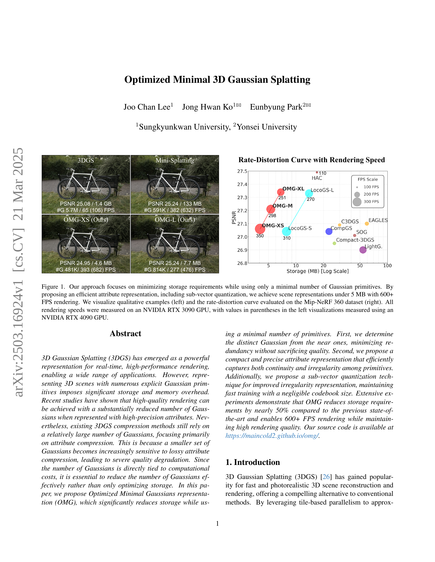
🔼 Figure 1 demonstrates the effectiveness of the proposed Optimized Minimal Gaussian (OMG) representation for 3D scenes. The left side shows qualitative results, comparing the visual quality of rendered scenes using OMG with other state-of-the-art methods. Note that the FPS values in parentheses were obtained using a more powerful NVIDIA RTX 4090 GPU. The right side presents a rate-distortion curve, illustrating the trade-off between storage size and PSNR (Peak Signal-to-Noise Ratio) achieved by OMG on the Mip-NeRF 360 benchmark dataset. This figure highlights OMG’s ability to achieve high-quality rendering with significantly reduced storage requirements (under 5 MB) and high frame rates (over 600 FPS) by optimizing both the number of Gaussian primitives and the efficiency of their attribute representation.
read the caption
Figure 1: Our approach focuses on minimizing storage requirements while using only a minimal number of Gaussian primitives. By proposing an efficient attribute representation, including sub-vector quantization, we achieve scene representations under 5 MB with 600+ FPS rendering. We visualize qualitative examples (left) and the rate-distortion curve evaluated on the Mip-NeRF 360 dataset (right). All rendering speeds were measured on an NVIDIA RTX 3090 GPU, with values in parentheses in the left visualizations measured using an NVIDIA RTX 4090 GPU.
| Mip-NeRF 360 | |||||
| Method | PSNR | SSIM | LPIPS | Size(MB) | FPS |
| 3DGS | 27.44 | 0.813 | 0.218 | 822.6 | 127 |
| Scaffold-GS [34] | 27.66 | 0.812 | 0.223 | 187.3 | 122 |
| CompGS [41] | 27.04 | 0.804 | 0.243 | 22.93 | 236 |
| Compact-3DGS [29] | 26.95 | 0.797 | 0.244 | 26.31 | 143 |
| C3DGS [42] | 27.09 | 0.802 | 0.237 | 29.98 | 134 |
| LightGaussian [11] | 26.90 | 0.800 | 0.240 | 53.96 | 244 |
| EAGLES [17] | 27.10 | 0.807 | 0.234 | 59.49 | 155 |
| SOG [39] | 27.01 | 0.800 | 0.226 | 43.77 | 134 |
| HAC [7] | 27.49 | 0.807 | 0.236 | 16.95 | 110 |
| LocoGS-S [50] | 27.04 | 0.806 | 0.232 | 7.90 | 310 |
| LocoGS-L [50] | 27.33 | 0.814 | 0.219 | 13.89 | 270 |
| OMG-XS | 27.06 | 0.807 | 0.243 | 4.06 | 350 (612) |
| OMG-M | 27.21 | 0.814 | 0.229 | 5.31 | 298 (511) |
| OMG-XL | 27.34 | 0.819 | 0.218 | 6.82 | 251 (416) |
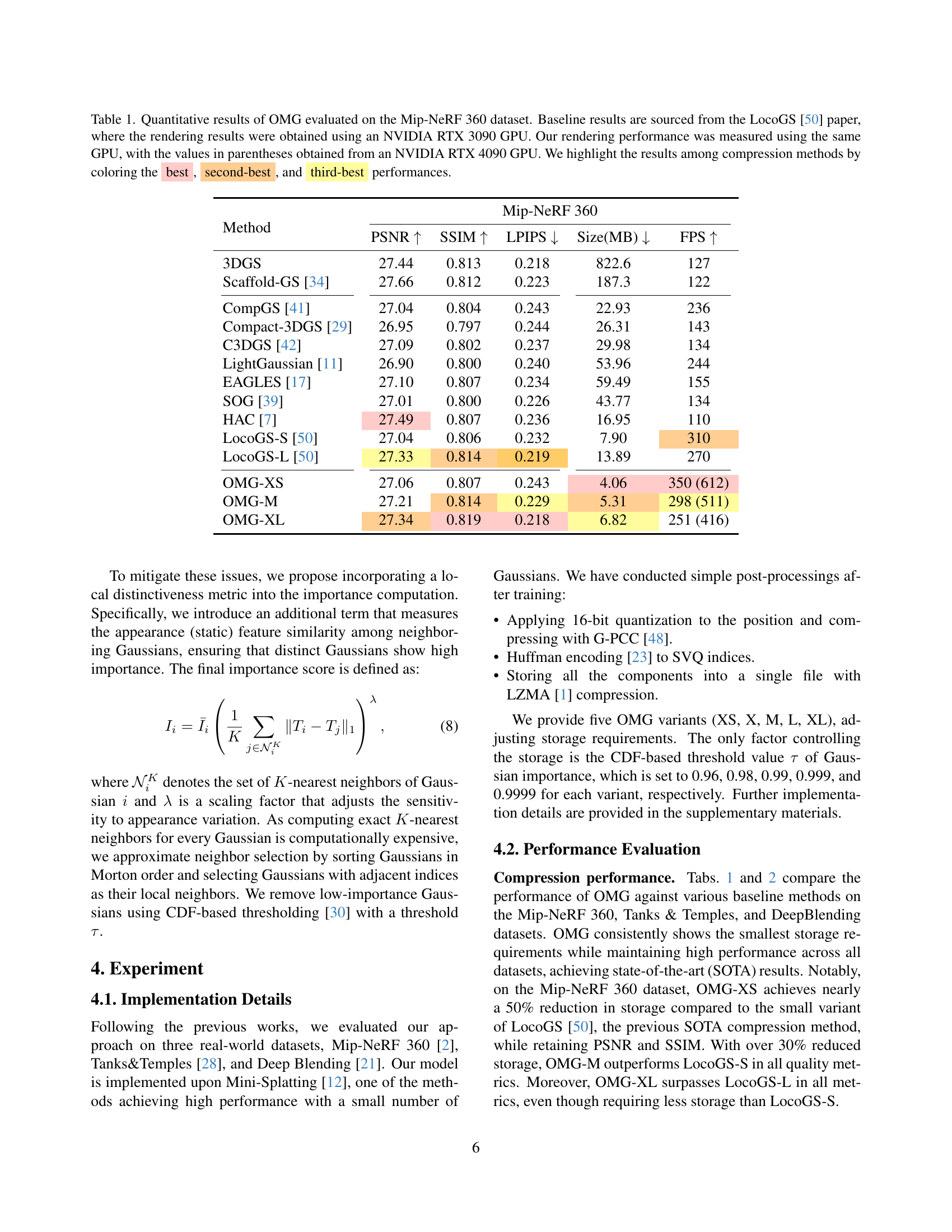
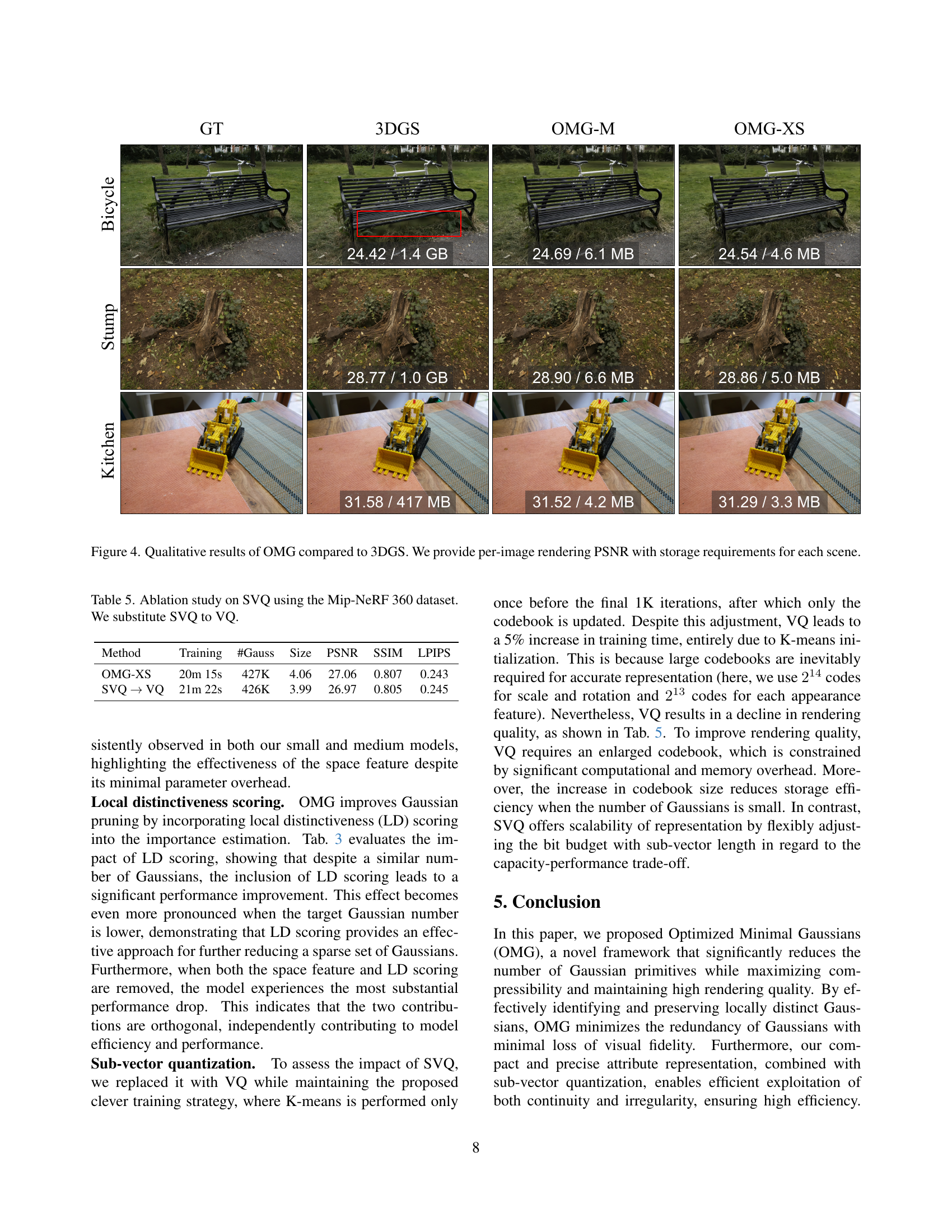
🔼 Table 1 presents a comparison of the proposed Optimized Minimal Gaussians (OMG) method against several state-of-the-art 3D Gaussian splatting techniques for scene representation on the Mip-NeRF 360 dataset. The table shows key metrics such as PSNR (Peak Signal-to-Noise Ratio), SSIM (Structural Similarity Index), LPIPS (Learned Perceptual Image Patch Similarity), model size in MB, and rendering speed in frames per second (FPS). The results for OMG are presented for various model sizes (XS, M, XL), demonstrating its scalability. Baseline values from the LocoGS paper are provided for comparison; the rendering performance reported in LocoGS was measured on an NVIDIA RTX 3090 GPU, and this table includes measurements on the same GPU plus additional measurements obtained with an NVIDIA RTX 4090 GPU for comparative purposes. The best, second-best, and third-best results among the different compression methods are highlighted in the table to easily see how OMG compares against other approaches.
read the caption
Table 1: Quantitative results of OMG evaluated on the Mip-NeRF 360 dataset. Baseline results are sourced from the LocoGS [50] paper, where the rendering results were obtained using an NVIDIA RTX 3090 GPU. Our rendering performance was measured using the same GPU, with the values in parentheses obtained from an NVIDIA RTX 4090 GPU. We highlight the results among compression methods by coloring the best, second-best, and third-best performances.
In-depth insights#
Minimal Gaussian#
The concept of “Minimal Gaussian” likely pertains to reducing the computational and storage burden associated with Gaussian representations, particularly in fields like 3D Gaussian Splatting (3DGS). The core idea revolves around optimizing the number of Gaussian primitives used to represent a scene or object. Instead of relying on a massive number of Gaussians, the focus shifts towards achieving comparable quality with a significantly smaller set. This necessitates efficient strategies for determining the most informative Gaussians and eliminating redundancy. Furthermore, it often involves employing compact and precise attribute representations to minimize the information required per Gaussian, ensuring that the reduced set can still accurately capture the complexity of the data. This involves balancing fidelity and efficiency to maintain visual quality while lowering computational costs.
OMG: Efficient 3D#
OMG: Efficient 3D likely refers to the core contribution of a research paper focused on optimizing 3D data representation or processing. It suggests a method that prioritizes efficiency, potentially in terms of storage, computation, or both. The name implies a significant improvement over existing techniques, perhaps aiming for minimal resource usage while maintaining acceptable quality. The method could involve novel compression strategies, data structures, or algorithms tailored to 3D data. We might anticipate that the OMG method could excel in scenarios where resources are constrained, such as mobile devices or real-time applications where speed is critical. Benchmarks against established methods will likely demonstrate the gains from OMG, and the paper would thoroughly analyze the trade-offs between efficiency and fidelity achieved by the OMG. This method would be suitable for areas where quick rendering is important.
SVQ Quantization#
Sub-Vector Quantization (SVQ) is introduced as a method to balance computational cost and storage efficiency. It partitions attribute vectors into sub-vectors, applying vector quantization separately to each. This allows for smaller codebooks and efficient lookups compared to standard vector quantization, which often requires large codebooks for high fidelity, leading to computational overhead. SVQ is applied to geometric attributes (scale and rotation) and appearance features, concatenating and splitting them as needed. A fine-tuning strategy is used in the final training iterations, freezing indices and fine-tuning codebooks to further improve efficiency. By reducing the dimensionality of each quantized unit, SVQ is able to maintain the high-precision representation.
Local Distinctness#
Local Distinctness is a crucial enhancement, improving Gaussian pruning by incorporating local feature similarity. This leads to significant performance gains, especially with a smaller Gaussian set, showcasing effectiveness in sparse scenarios. The impact becomes prominent with lower target Gaussian numbers. Removing both spatial features and local features causes a significant performance drop. This shows the two parts works independently and are important to model performance and efficiency.
Low Storage NeRF#
Low-storage NeRF aims to reduce the memory footprint of Neural Radiance Fields (NeRFs) without significantly sacrificing rendering quality. This involves techniques like parameter compression, knowledge distillation, and efficient data structures. The goal is to enable NeRFs on resource-constrained devices or to facilitate the storage and transmission of large-scale 3D scenes. The challenge lies in balancing compression with the need to preserve the intricate details and view-dependent effects captured by the original NeRF model. Approaches often involve quantization, pruning redundant parameters, or representing the scene with a more compact set of basis functions. Careful design is crucial to maintain visual fidelity and rendering speed while achieving significant storage savings.
More visual insights#
More on figures
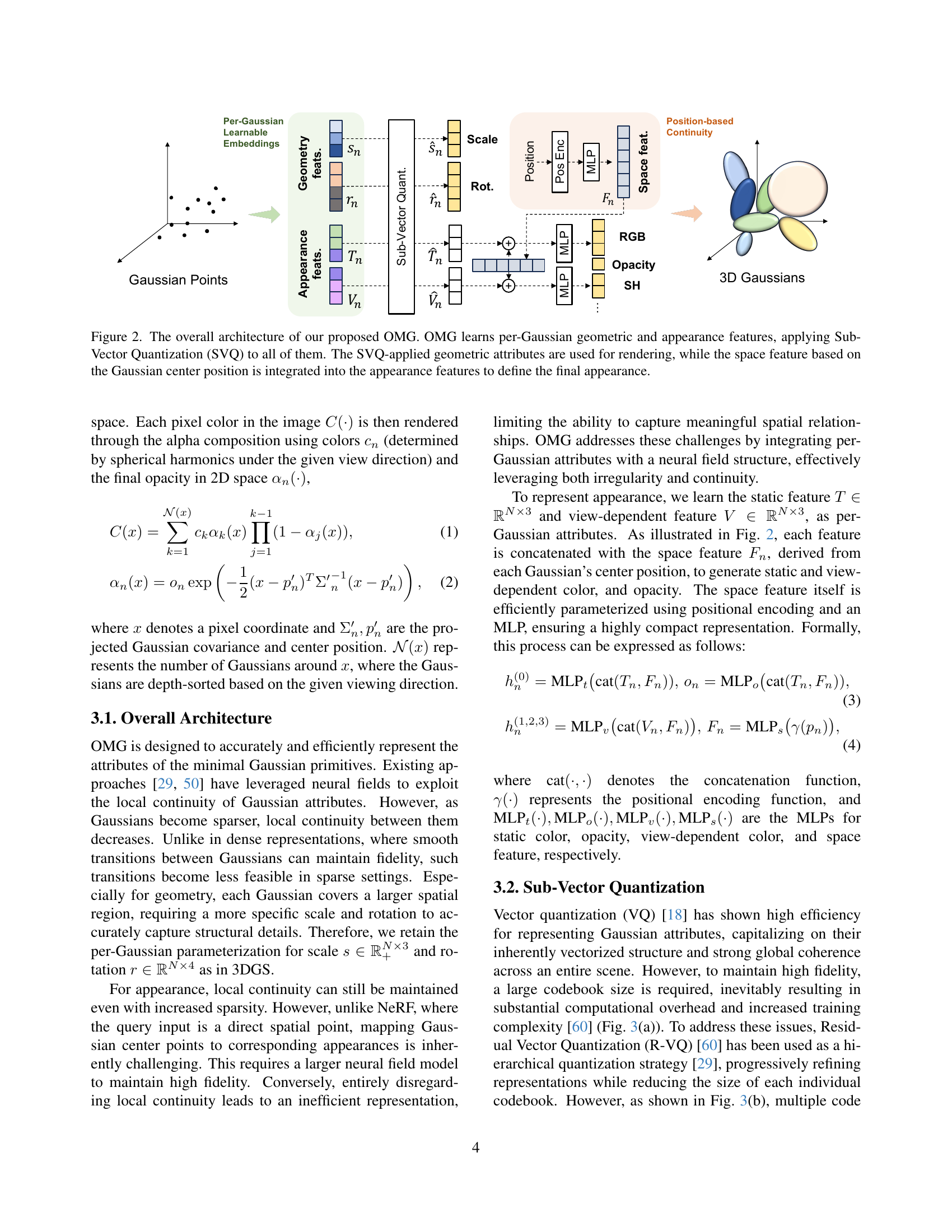
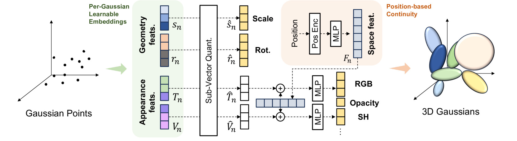
🔼 This figure illustrates the architecture of the Optimized Minimal Gaussians (OMG) model. The OMG model efficiently represents 3D scenes using a minimal number of Gaussian primitives. It learns both geometric (position, scale, rotation) and appearance (static and view-dependent color, opacity) features for each Gaussian. These features are then compressed using Sub-Vector Quantization (SVQ) to reduce storage. The geometric attributes (after SVQ) are used directly for rendering. A novel spatial feature, derived from the Gaussian’s position, is incorporated into the appearance features to improve rendering quality, particularly in areas with sparse Gaussians. This combination balances the need for compact representation with accurate rendering.
read the caption
Figure 2: The overall architecture of our proposed OMG. OMG learns per-Gaussian geometric and appearance features, applying Sub-Vector Quantization (SVQ) to all of them. The SVQ-applied geometric attributes are used for rendering, while the space feature based on the Gaussian center position is integrated into the appearance features to define the final appearance.

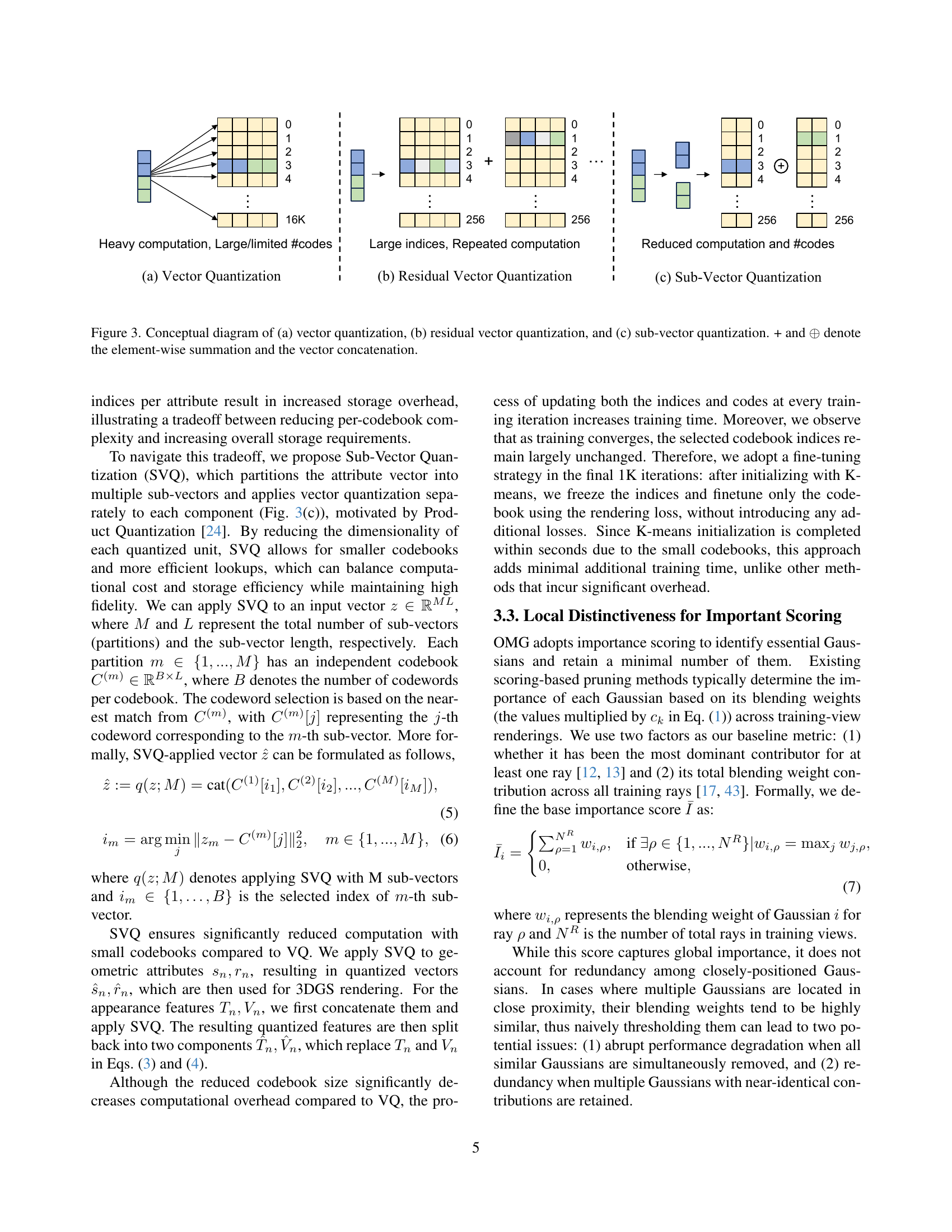
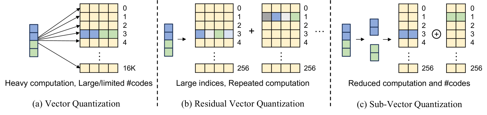
🔼 This figure illustrates three different vector quantization methods used for compressing Gaussian attributes in 3D Gaussian splatting. (a) shows standard vector quantization, where the entire attribute vector is encoded using a single codebook. (b) depicts residual vector quantization, which involves multiple stages of encoding where the residuals from previous stages are encoded. (c) presents sub-vector quantization, which partitions the attribute vector into multiple sub-vectors and uses separate codebooks for each, reducing the computational complexity of large codebooks while maintaining precision. The ‘+’ symbol represents element-wise summation, and the ‘⊕’ symbol denotes vector concatenation.
read the caption
Figure 3: Conceptual diagram of (a) vector quantization, (b) residual vector quantization, and (c) sub-vector quantization. + and ⊕direct-sum\oplus⊕ denote the element-wise summation and the vector concatenation.
More on tables
| Tank&Temples | Deep Blending | |||||||||
|---|---|---|---|---|---|---|---|---|---|---|
| Method | PSNR | SSIM | LPIPS | Size | FPS | PSNR | SSIM | LPIPS | Size | FPS |
| 3DGS [26] | 23.67 | 0.844 | 0.179 | 452.4 | 175 | 29.48 | 0.900 | 0.246 | 692.5 | 134 |
| Scaffold-GS [34] | 24.11 | 0.855 | 0.165 | 154.3 | 109 | 30.28 | 0.907 | 0.243 | 121.2 | 194 |
| CompGS [41] | 23.29 | 0.835 | 0.201 | 14.23 | 329 | 29.89 | 0.907 | 0.253 | 15.15 | 301 |
| Compact-3DGS [29] | 23.33 | 0.831 | 0.202 | 18.97 | 199 | 29.71 | 0.901 | 0.257 | 21.75 | 184 |
| C3DGS [42] | 23.52 | 0.837 | 0.188 | 18.58 | 166 | 29.53 | 0.899 | 0.254 | 24.96 | 143 |
| LightGaussian [11] | 23.32 | 0.829 | 0.204 | 29.94 | 379 | 29.12 | 0.895 | 0.262 | 45.25 | 287 |
| EAGLES [17] | 23.14 | 0.833 | 0.203 | 30.18 | 244 | 29.72 | 0.906 | 0.249 | 54.45 | 137 |
| SOG [39] | 23.54 | 0.833 | 0.188 | 24.42 | 222 | 29.21 | 0.891 | 0.271 | 19.32 | 224 |
| HAC [7] | 24.08 | 0.846 | 0.186 | 8.42 | 129 | 29.99 | 0.902 | 0.268 | 4.51 | 235 |
| LocoGS-S [50] | 23.63 | 0.847 | 0.169 | 6.59 | 333 | 30.06 | 0.904 | 0.249 | 7.64 | 334 |
| OMG-M | 23.52 | 0.842 | 0.189 | 3.22 | 555 (887) | 29.77 | 0.908 | 0.253 | 4.34 | 524 (894) |
| OMG-L | 23.60 | 0.846 | 0.181 | 3.93 | 478 (770) | 29.88 | 0.910 | 0.247 | 5.21 | 479 (810) |
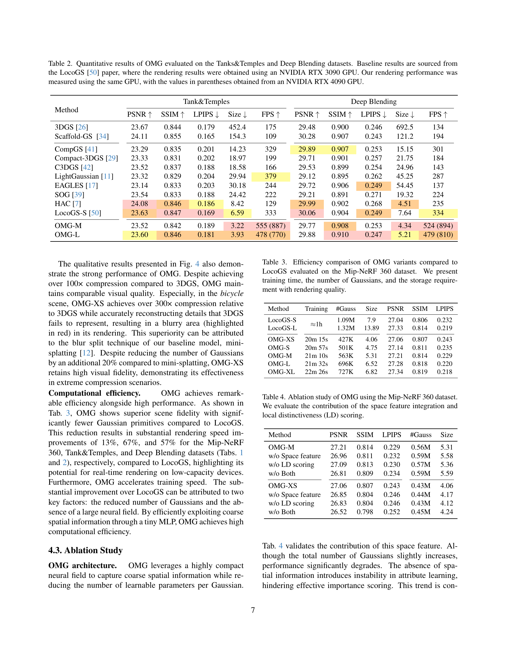
🔼 Table 2 presents a comparison of the performance of the Optimized Minimal Gaussians (OMG) method against several baseline methods on two datasets: Tanks & Temples and Deep Blending. The metrics used for comparison include PSNR, SSIM, LPIPS, size (in MB), and FPS. For each method, the table shows the results obtained using an NVIDIA RTX 3090 GPU, which is consistent with the LocoGS [50] paper used as a baseline. Additionally, to provide a more comprehensive evaluation, the table also includes performance results measured using a higher-performance NVIDIA RTX 4090 GPU, which is indicated by values in parentheses. This allows for better understanding of the relative performance gains across different hardware.
read the caption
Table 2: Quantitative results of OMG evaluated on the Tanks&Temples and Deep Blending datasets. Baseline results are sourced from the LocoGS [50] paper, where the rendering results were obtained using an NVIDIA RTX 3090 GPU. Our rendering performance was measured using the same GPU, with the values in parentheses obtained from an NVIDIA RTX 4090 GPU.
| Method | Training | #Gauss | Size | PSNR | SSIM | LPIPS |
|---|---|---|---|---|---|---|
| LocoGS-S | 1h | 1.09M | 7.9 | 27.04 | 0.806 | 0.232 |
| LocoGS-L | 1.32M | 13.89 | 27.33 | 0.814 | 0.219 | |
| OMG-XS | 20m 15s | 427K | 4.06 | 27.06 | 0.807 | 0.243 |
| OMG-S | 20m 57s | 501K | 4.75 | 27.14 | 0.811 | 0.235 |
| OMG-M | 21m 10s | 563K | 5.31 | 27.21 | 0.814 | 0.229 |
| OMG-L | 21m 32s | 696K | 6.52 | 27.28 | 0.818 | 0.220 |
| OMG-XL | 22m 26s | 727K | 6.82 | 27.34 | 0.819 | 0.218 |
🔼 This table compares the efficiency of different variants of the Optimized Minimal Gaussians (OMG) representation with the state-of-the-art LocoGS method on the Mip-NeRF 360 dataset. It shows a comparison of training time, the number of Gaussian primitives used, the resulting storage size, and the rendering quality (PSNR, SSIM, LPIPS) for each method. This allows for a quantitative assessment of the trade-offs between model complexity, storage efficiency, and rendering quality.
read the caption
Table 3: Efficiency comparison of OMG variants compared to LocoGS evaluated on the Mip-NeRF 360 dataset. We present training time, the number of Gaussians, and the storage requirement with rendering quality.
| Method | PSNR | SSIM | LPIPS | #Gauss | Size |
|---|---|---|---|---|---|
| OMG-M | 27.21 | 0.814 | 0.229 | 0.56M | 5.31 |
| w/o Space feature | 26.96 | 0.811 | 0.232 | 0.59M | 5.58 |
| w/o LD scoring | 27.09 | 0.813 | 0.230 | 0.57M | 5.36 |
| w/o Both | 26.81 | 0.809 | 0.234 | 0.59M | 5.59 |
| OMG-XS | 27.06 | 0.807 | 0.243 | 0.43M | 4.06 |
| w/o Space feature | 26.85 | 0.804 | 0.246 | 0.44M | 4.17 |
| w/o LD scoring | 26.83 | 0.804 | 0.246 | 0.43M | 4.12 |
| w/o Both | 26.52 | 0.798 | 0.252 | 0.45M | 4.24 |
🔼 This table presents an ablation study on the Optimized Minimal Gaussians (OMG) model, specifically examining the impact of two key components: the space feature integration and the local distinctiveness (LD) scoring. It uses the Mip-NeRF 360 dataset for evaluation and shows the PSNR, SSIM, LPIPS metrics, the number of Gaussians, and the model size for different configurations of OMG. The configurations vary based on the inclusion or exclusion of the space feature and LD scoring, allowing for a quantitative assessment of their individual contributions to the overall performance of the OMG model.
read the caption
Table 4: Ablation study of OMG using the Mip-NeRF 360 dataset. We evaluate the contribution of the space feature integration and local distinctiveness (LD) scoring.
| Method | Training | #Gauss | Size | PSNR | SSIM | LPIPS |
|---|---|---|---|---|---|---|
| OMG-XS | 20m 15s | 427K | 4.06 | 27.06 | 0.807 | 0.243 |
| SVQ VQ | 21m 22s | 426K | 3.99 | 26.97 | 0.805 | 0.245 |
🔼 This ablation study analyzes the impact of using Sub-Vector Quantization (SVQ) versus Vector Quantization (VQ) in the Optimized Minimal Gaussians (OMG) model. The experiment focuses on the Mip-NeRF 360 dataset. The table compares performance metrics (Training time, number of Gaussians, model Size, PSNR, SSIM, LPIPS) for OMG-XS with SVQ and the same model but with SVQ replaced by VQ. This allows for a direct comparison of the two quantization methods and reveals the effects on model performance and training efficiency.
read the caption
Table 5: Ablation study on SVQ using the Mip-NeRF 360 dataset. We substitute SVQ to VQ.
| G-PCC | Huffman | Size (MB) |
|---|---|---|
| - | - | 5.82 |
| ✓ | - | 4.30 |
| - | ✓ | 5.58 |
| OMG-XS | 4.06 | |
| - | - | 6.83 |
| ✓ | - | 5.04 |
| - | ✓ | 6.54 |
| OMG-S | 4.75 | |
| - | - | 7.66 |
| ✓ | - | 5.64 |
| - | ✓ | 7.33 |
| OMG-M | 5.31 | |
| - | - | 9.47 |
| ✓ | - | 6.92 |
| - | ✓ | 9.08 |
| OMG-L | 6.52 | |
| - | - | 9.89 |
| ✓ | - | 7.25 |
| - | ✓ | 9.46 |
| OMG-XL | 6.82 | |
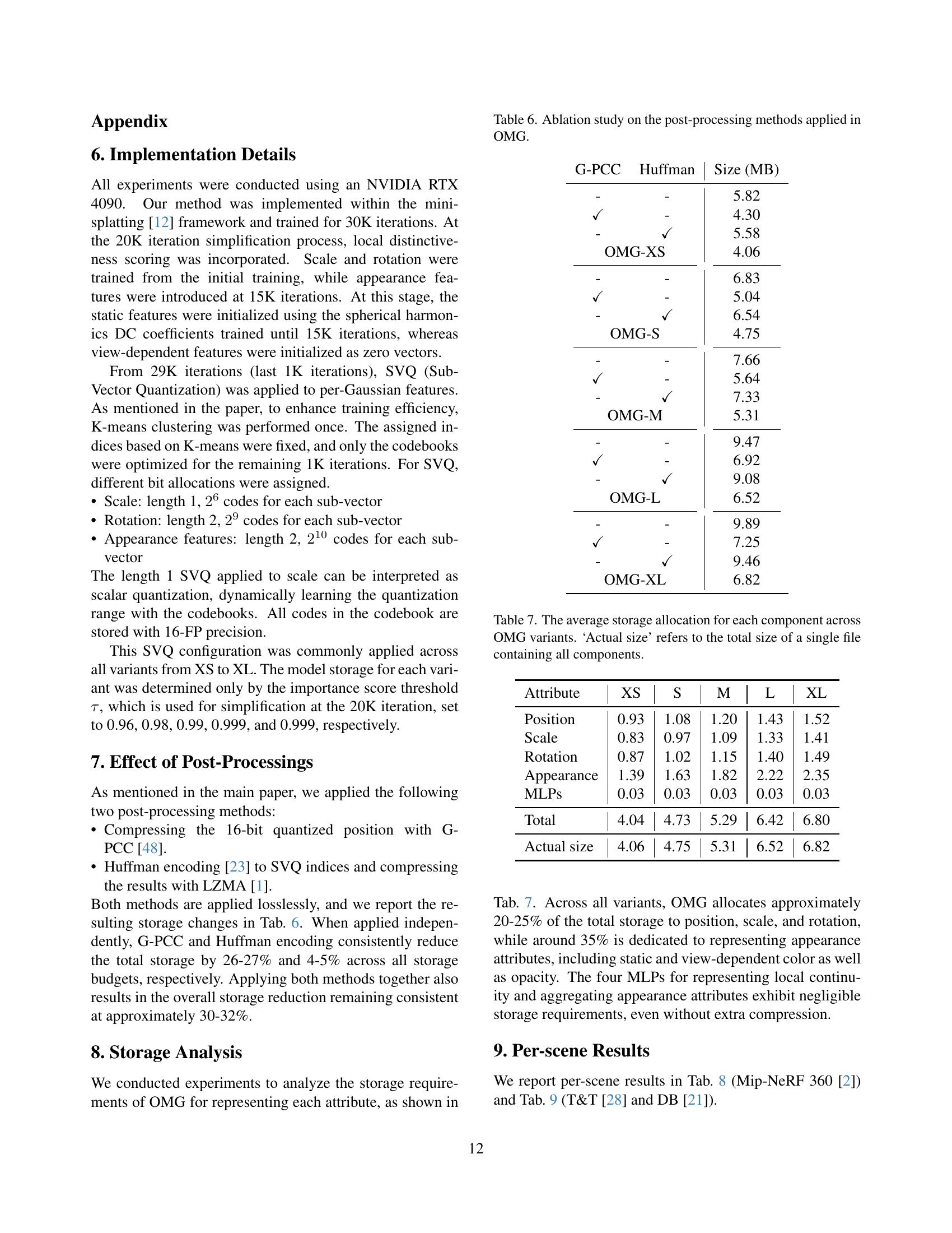
🔼 This table presents an ablation study analyzing the impact of different post-processing techniques on the overall size of the Optimized Minimal Gaussians (OMG) model. It shows the model sizes resulting from using various combinations of G-PCC compression, Huffman coding, and LZMA compression. This allows assessment of the effectiveness of each compression method independently and in combination.
read the caption
Table 6: Ablation study on the post-processing methods applied in OMG.
| Attribute | XS | S | M | L | XL |
|---|---|---|---|---|---|
| Position | 0.93 | 1.08 | 1.20 | 1.43 | 1.52 |
| Scale | 0.83 | 0.97 | 1.09 | 1.33 | 1.41 |
| Rotation | 0.87 | 1.02 | 1.15 | 1.40 | 1.49 |
| Appearance | 1.39 | 1.63 | 1.82 | 2.22 | 2.35 |
| MLPs | 0.03 | 0.03 | 0.03 | 0.03 | 0.03 |
| Total | 4.04 | 4.73 | 5.29 | 6.42 | 6.80 |
| Actual size | 4.06 | 4.75 | 5.31 | 6.52 | 6.82 |
🔼 This table details the average storage used by each component (position, scale, rotation, appearance features, and MLPs) within the Optimized Minimal Gaussians (OMG) model. Different versions of the OMG model (XS, S, M, L, XL) are compared, showing how storage needs vary with model complexity. The ‘Actual size’ column represents the total file size for each model variant, encompassing all components.
read the caption
Table 7: The average storage allocation for each component across OMG variants. ‘Actual size’ refers to the total size of a single file containing all components.
| Method | Metric | bicycle | bonsai | counter | flowers | garden | kitchen | room | stump | treehill | Avg. |
|---|---|---|---|---|---|---|---|---|---|---|---|
| OMG-XS | PSNR | 24.95 | 30.90 | 28.40 | 21.32 | 26.42 | 30.81 | 31.09 | 27.00 | 22.60 | 27.06 |
| SSIM | 0.743 | 0.932 | 0.899 | 0.596 | 0.818 | 0.919 | 0.918 | 0.788 | 0.647 | 0.807 | |
| LPIPS | 0.276 | 0.202 | 0.206 | 0.368 | 0.190 | 0.137 | 0.208 | 0.247 | 0.357 | 0.243 | |
| Train | 18:03 | 20:30 | 24:44 | 19:18 | 18:02 | 23:45 | 20:30 | 17:49 | 19:40 | 20:15 | |
| #Gauss | 480772 | 263892 | 310056 | 543034 | 607254 | 356752 | 281236 | 523821 | 479520 | 427371 | |
| Size | 4.61 | 2.53 | 2.95 | 5.24 | 5.65 | 3.33 | 2.67 | 4.95 | 4.64 | 4.06 | |
| FPS | 682 | 648 | 433 | 616 | 615 | 498 | 648 | 708 | 658 | 612 | |
| OMG-S | PSNR | 25.08 | 31.05 | 28.56 | 21.18 | 26.56 | 30.89 | 31.20 | 27.08 | 22.64 | 27.14 |
| SSIM | 0.750 | 0.936 | 0.903 | 0.602 | 0.826 | 0.921 | 0.922 | 0.792 | 0.650 | 0.811 | |
| LPIPS | 0.264 | 0.195 | 0.199 | 0.358 | 0.177 | 0.132 | 0.201 | 0.239 | 0.347 | 0.235 | |
| Train | 19:01 | 21:09 | 25:19 | 20:13 | 18:41 | 24:12 | 21:38 | 18:29 | 19:55 | 20:57 | |
| #Gauss | 573126 | 310096 | 360930 | 633607 | 691441 | 412126 | 338884 | 619734 | 573425 | 501485 | |
| Size | 5.46 | 2.94 | 3.41 | 6.10 | 6.43 | 3.83 | 3.19 | 5.83 | 5.54 | 4.75 | |
| FPS | 601 | 585 | 401 | 555 | 556 | 462 | 620 | 601 | 588 | 552 | |
| OMG-M | PSNR | 25.14 | 31.06 | 28.62 | 21.40 | 26.71 | 31.05 | 31.30 | 27.06 | 22.55 | 27.21 |
| SSIM | 0.756 | 0.938 | 0.905 | 0.606 | 0.832 | 0.923 | 0.923 | 0.794 | 0.652 | 0.814 | |
| LPIPS | 0.256 | 0.190 | 0.195 | 0.351 | 0.169 | 0.129 | 0.198 | 0.233 | 0.339 | 0.229 | |
| Train | 18:58 | 21:01 | 25:44 | 20:35 | 18:51 | 24:18 | 22:14 | 18:31 | 20:22 | 21:10 | |
| #Gauss | 646191 | 350999 | 400442 | 708074 | 772338 | 454908 | 375520 | 704907 | 649157 | 562504 | |
| Size | 6.15 | 3.33 | 3.76 | 6.79 | 7.18 | 4.21 | 3.53 | 6.61 | 6.24 | 5.31 | |
| FPS | 562 | 536 | 371 | 510 | 522 | 440 | 566 | 566 | 525 | 511 | |
| OMG-L | PSNR | 25.24 | 31.47 | 28.66 | 21.45 | 26.83 | 31.03 | 31.26 | 27.05 | 22.57 | 27.28 |
| SSIM | 0.762 | 0.941 | 0.907 | 0.613 | 0.837 | 0.924 | 0.926 | 0.795 | 0.653 | 0.818 | |
| LPIPS | 0.241 | 0.183 | 0.189 | 0.338 | 0.160 | 0.126 | 0.191 | 0.226 | 0.329 | 0.220 | |
| Train | 19:25 | 21:16 | 26:06 | 20:50 | 19:14 | 24:20 | 22:05 | 19:22 | 21:14 | 21:32 | |
| #Gauss | 813561 | 463285 | 480133 | 859963 | 909961 | 524457 | 524457 | 869388 | 819435 | 696071 | |
| Size | 7.69 | 4.32 | 4.48 | 8.23 | 8.42 | 4.82 | 4.82 | 8.14 | 7.81 | 6.52 | |
| FPS | 476 | 492 | 332 | 422 | 422 | 405 | 539 | 468 | 414 | 441 | |
| OMG-XL | PSNR | 25.22 | 31.51 | 28.78 | 21.52 | 26.93 | 31.15 | 31.25 | 27.00 | 22.69 | 27.34 |
| SSIM | 0.764 | 0.942 | 0.908 | 0.614 | 0.839 | 0.925 | 0.926 | 0.796 | 0.655 | 0.819 | |
| LPIPS | 0.239 | 0.182 | 0.187 | 0.334 | 0.157 | 0.126 | 0.191 | 0.224 | 0.324 | 0.218 | |
| Train | 20:43 | 21:54 | 26:21 | 22:09 | 20:23 | 24:56 | 22:37 | 20:22 | 22:33 | 22:26 | |
| #Gauss | 864124 | 450246 | 507473 | 922061 | 953050 | 547636 | 493754 | 920589 | 885229 | 727129 | |
| Size | 8.15 | 4.22 | 4.72 | 8.81 | 8.82 | 5.02 | 4.58 | 8.59 | 8.44 | 6.82 | |
| FPS | 430 | 465 | 324 | 379 | 422 | 397 | 512 | 435 | 384 | 416 |
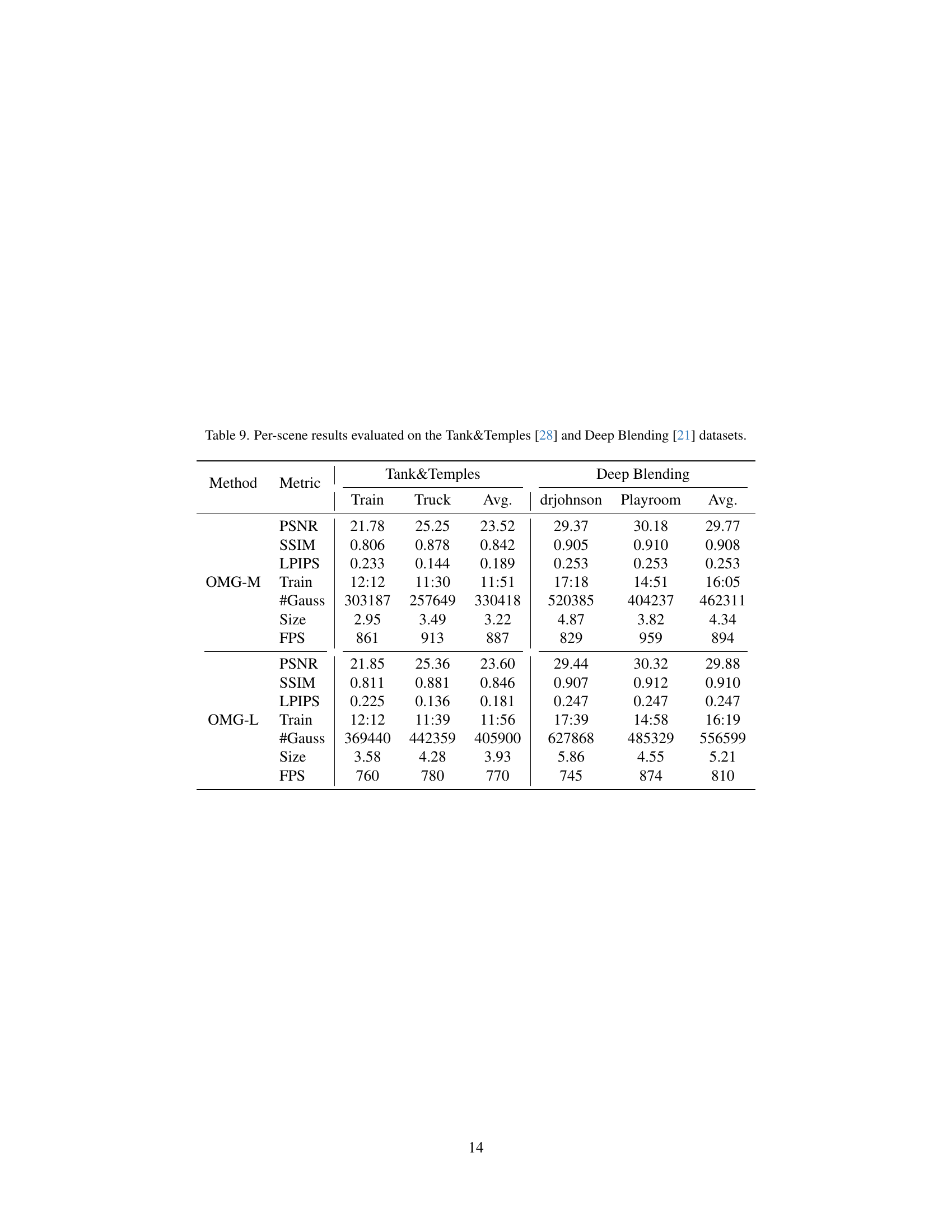
🔼 This table presents a comprehensive breakdown of the per-scene performance metrics obtained from evaluating the Optimized Minimal Gaussians (OMG) model on the Mip-NeRF 360 dataset. It details the PSNR, SSIM, and LPIPS values for various scenes (bicycle, bonsai, counter, flowers, garden, kitchen, room, stump, treehill) across different configurations of the OMG model (OMG-XS, OMG-S, OMG-M, OMG-L, OMG-XL). In addition to the image quality metrics, the table includes the training time, the number of Gaussians used, the model size (in MB), and the rendering FPS for each scene and model variant. This allows for a detailed comparison of the trade-offs between model size, computational cost, and visual fidelity across different scenes and OMG configurations.
read the caption
Table 8: Per-scene results evaluated on the Mip-NeRF 360 [2] dataset.
| Method | Metric | Tank&Temples | Deep Blending | ||||
|---|---|---|---|---|---|---|---|
| Train | Truck | Avg. | drjohnson | Playroom | Avg. | ||
| OMG-M | PSNR | 21.78 | 25.25 | 23.52 | 29.37 | 30.18 | 29.77 |
| SSIM | 0.806 | 0.878 | 0.842 | 0.905 | 0.910 | 0.908 | |
| LPIPS | 0.233 | 0.144 | 0.189 | 0.253 | 0.253 | 0.253 | |
| Train | 12:12 | 11:30 | 11:51 | 17:18 | 14:51 | 16:05 | |
| #Gauss | 303187 | 257649 | 330418 | 520385 | 404237 | 462311 | |
| Size | 2.95 | 3.49 | 3.22 | 4.87 | 3.82 | 4.34 | |
| FPS | 861 | 913 | 887 | 829 | 959 | 894 | |
| OMG-L | PSNR | 21.85 | 25.36 | 23.60 | 29.44 | 30.32 | 29.88 |
| SSIM | 0.811 | 0.881 | 0.846 | 0.907 | 0.912 | 0.910 | |
| LPIPS | 0.225 | 0.136 | 0.181 | 0.247 | 0.247 | 0.247 | |
| Train | 12:12 | 11:39 | 11:56 | 17:39 | 14:58 | 16:19 | |
| #Gauss | 369440 | 442359 | 405900 | 627868 | 485329 | 556599 | |
| Size | 3.58 | 4.28 | 3.93 | 5.86 | 4.55 | 5.21 | |
| FPS | 760 | 780 | 770 | 745 | 874 | 810 | |
🔼 This table presents a detailed breakdown of the performance of the Optimized Minimal Gaussians (OMG) model on a per-scene basis for two datasets: Tanks & Temples and Deep Blending. For each scene within each dataset, the table provides key metrics such as PSNR, SSIM, and LPIPS, offering a comprehensive evaluation of the visual quality achieved by the model. Additionally, the training time, the number of Gaussians utilized, the overall file size, and the frames per second (FPS) achieved during rendering are reported, providing a complete picture of both the model’s accuracy and efficiency.
read the caption
Table 9: Per-scene results evaluated on the Tank&Temples [28] and Deep Blending [21] datasets.
Full paper#