TL;DR#
Fast camera motions cause motion blur, which makes existing methods to estimate camera pose fails. Conventional approaches often discard blurred frames or rely on inertial measurement units (IMUs). This introduces challenges like sensor synchronization and drift. Therefore, motion blur has always been viewed as unwanted artifact.
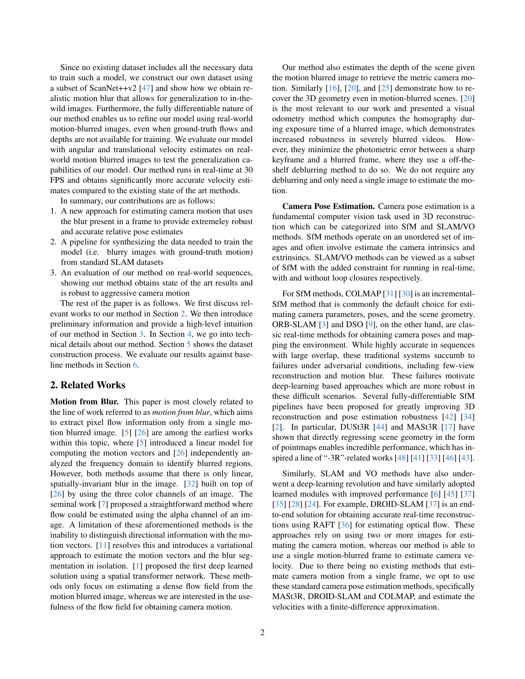
This paper introduces a novel approach: using motion blur as a cue for estimating camera motion. The method involves predicting a dense motion flow field and a monocular depth map from a single motion-blurred image. The instantaneous camera velocity is then recovered by solving a linear least squares problem. This creates an IMU-like measurement robust to fast movements. The model is trained on a new large-scale synthetic dataset and refined on real data using a fully differentiable pipeline.
Key Takeaways#
Why does it matter?#
This paper introduces an innovative method for motion estimation, leveraging motion blur as a cue rather than a hindrance. It also contributes a new dataset and a differentiable pipeline, achieving state-of-the-art results and opening new avenues for research in motion estimation and visual odometry.
Visual Insights#

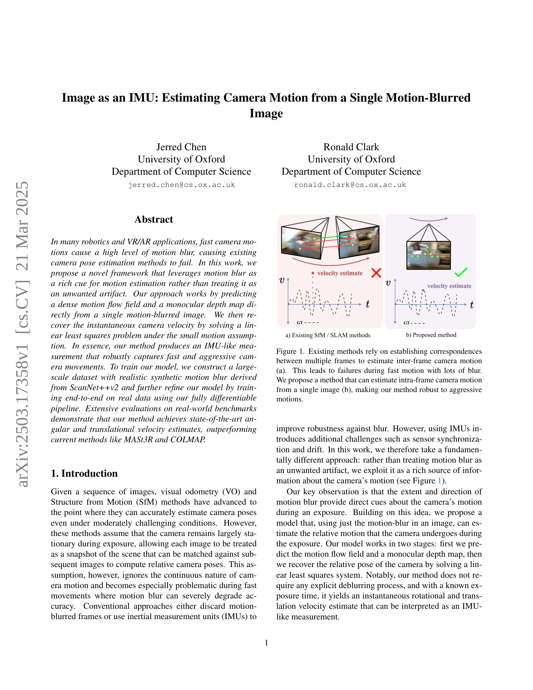
🔼 Figure 1 illustrates the difference between traditional visual odometry/SLAM methods and the proposed method. Traditional methods (a) rely on feature matching between multiple frames to compute camera motion. However, this approach fails when significant motion blur is present during fast camera movements. The proposed method (b) directly estimates camera motion from a single motion-blurred image by exploiting motion blur as a cue, enabling robust estimation even under aggressive motions.
read the caption
Figure 1: Existing methods rely on establishing correspondences between multiple frames to estimate inter-frame camera motion (a). This leads to failures during fast motion with lots of blur. We propose a method that can estimate intra-frame camera motion from a single image (b), making our method robust to aggressive motions.
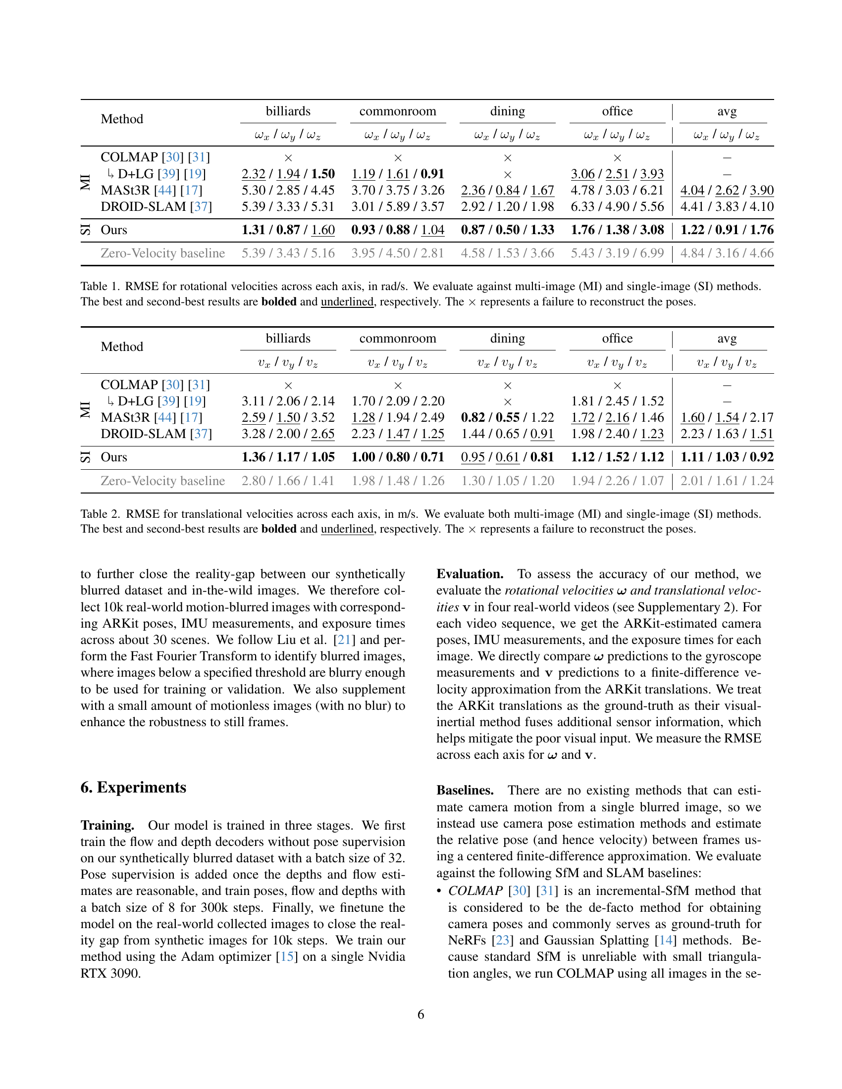
| Method | billiards | commonroom | dining | office | avg | |
|---|---|---|---|---|---|---|
| / / | / / | / / | / / | / / | ||
| MI | COLMAP [30] [31] | |||||
| D+LG [39] [19] | 2.32 / 1.94 / 1.50 | 1.19 / 1.61 / 0.91 | 3.06 / 2.51 / 3.93 | |||
| MASt3R [44] [17] | 5.30 / 2.85 / 4.45 | 3.70 / 3.75 / 3.26 | 2.36 / 0.84 / 1.67 | 4.78 / 3.03 / 6.21 | 4.04 / 2.62 / 3.90 | |
| DROID-SLAM [37] | 5.39 / 3.33 / 5.31 | 3.01 / 5.89 / 3.57 | 2.92 / 1.20 / 1.98 | 6.33 / 4.90 / 5.56 | 4.41 / 3.83 / 4.10 | |
SI | Ours | 1.31 / 0.87 / 1.60 | 0.93 / 0.88 / 1.04 | 0.87 / 0.50 / 1.33 | 1.76 / 1.38 / 3.08 | 1.22 / 0.91 / 1.76 |
| Zero-Velocity baseline | 5.39 / 3.43 / 5.16 | 3.95 / 4.50 / 2.81 | 4.58 / 1.53 / 3.66 | 5.43 / 3.19 / 6.99 | 4.84 / 3.16 / 4.66 |
🔼 This table presents the Root Mean Squared Error (RMSE) for rotational velocities along the x, y, and z axes, measured in radians per second (rad/s). The performance of several methods is compared, categorized as either multi-image (MI) methods or single-image (SI) methods, reflecting whether the methods process multiple images or a single image for pose estimation. The best and second-best results for each method are highlighted using bold and underlined font respectively. An ‘x’ indicates that a method failed to reconstruct camera poses for a particular scene.
read the caption
Table 1: RMSE for rotational velocities across each axis, in rad/s. We evaluate against multi-image (MI) and single-image (SI) methods. The best and second-best results are bolded and underlined, respectively. The ×\times× represents a failure to reconstruct the poses.
In-depth insights#
Blur as Motion#
The idea of leveraging motion blur as a cue for understanding camera movement represents a significant shift in perspective. Traditionally, blur is seen as an artifact to be removed, but recent research suggests its potential as a valuable source of information. Motion blur directly reflects the camera’s trajectory during the exposure time, offering insights into both the speed and direction of movement. This approach could be particularly beneficial in scenarios where traditional visual odometry or SLAM methods struggle due to insufficient texture or rapid motion. Extracting reliable motion information from blur requires sophisticated techniques to disentangle the effects of scene geometry, camera motion, and the blurring process itself. Advanced algorithms can be developed to estimate camera motion parameters directly from the blurred image, potentially achieving robustness against challenging conditions. By exploiting blur as an informative cue, it might be possible to create more resilient and accurate systems for visual navigation, robotics, and augmented reality applications.
IMU-like Vision#
The idea of “IMU-like Vision” is intriguing, aiming to derive motion information directly from visual data akin to how an Inertial Measurement Unit (IMU) functions. This approach seeks to extract instantaneous velocity and angular rate from images, bypassing traditional methods. The paper effectively turns motion blur into a valuable cue, potentially eliminating the need for IMUs in some applications. It’s a significant shift from treating motion blur as an artifact to actively leveraging it. It enables robust camera motion estimates even in challenging, fast-motion scenarios where conventional methods falter. By extracting a dense motion flow field from motion-blurred images, it provides the relative motion of the camera, yielding an instantaneous rotational and translation velocity, directly providing IMU-like measurements robust to fast and aggressive movements.
Differentiable Solver#
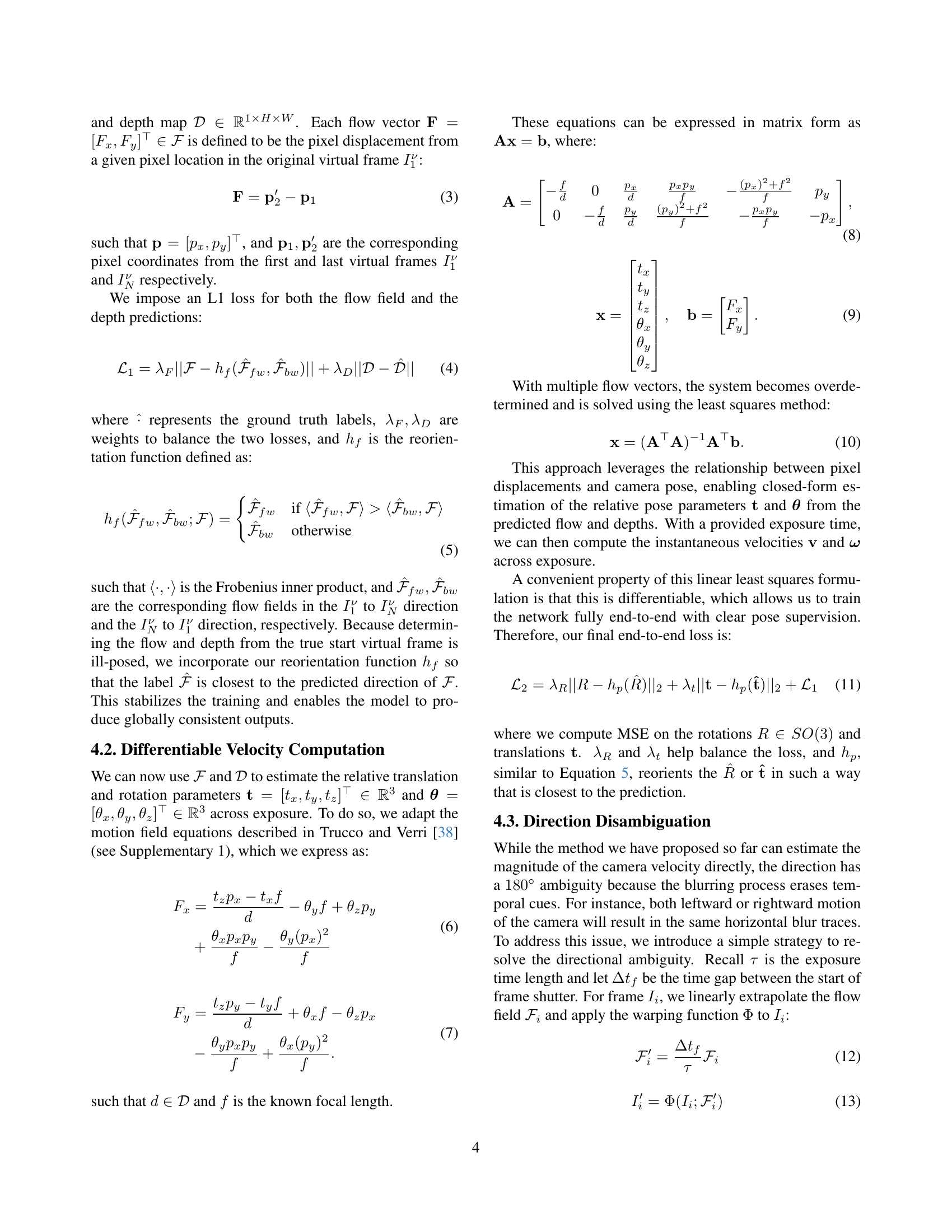
While the heading ‘Differentiable Solver’ isn’t explicitly present, the paper extensively employs differentiable techniques. Crucially, the method utilizes a differentiable least squares solver to recover camera velocity from predicted flow and depth. This differentiability is vital, enabling end-to-end training of the entire network, including the velocity estimation process, with pose supervision. The network can directly learn to predict flow and depth representations that are most suitable for accurate camera motion estimation. Without the differentiability, the velocity solver would act as a non-differentiable bottleneck, preventing the gradients from flowing back to the flow and depth prediction modules. The reorientation function helps stabilize the training, allowing for consistent output. It provides clear pose supervision, which is important for obtaining optimal solutions.
Real-world Robust#
The notion of ‘Real-world Robust’ in a research paper, especially in areas like computer vision or robotics, typically refers to the ability of a proposed method or system to perform reliably and accurately when deployed in uncontrolled, everyday environments. This is a crucial aspect of any practical application. Demonstrating real-world robustness often involves testing the system under a variety of challenging conditions that are commonly encountered outside of a lab setting. These might include variations in lighting, occlusions, noisy sensor data, unexpected object appearances, and dynamic environments. The evaluation metrics used to assess robustness would likely go beyond simple accuracy measurements and incorporate aspects like reliability, failure rate, and adaptability to unforeseen circumstances.A system that is ‘Real-world Robust’ should be able to gracefully handle these challenges, maintaining acceptable performance even when faced with imperfect or incomplete data. This requires careful consideration of factors such as sensor noise, calibration errors, and the limitations of the underlying algorithms. Techniques such as data augmentation, robust optimization methods, and adaptive filtering can be employed to improve the system’s resilience to real-world conditions. The ultimate goal is to create a system that can operate reliably and effectively in the complex and unpredictable environments that characterize real-world applications. A rigorous evaluation on diverse datasets is important.
No Deblurring#
The “No Deblurring” aspect of this paper is a key innovation. Instead of attempting to remove motion blur, which is a difficult and often imperfect process, the method explicitly leverages the blur as a source of information. Traditional approaches treat blur as noise, discarding blurred frames or trying to computationally reverse the blurring effect. This work inverts that paradigm, recognizing that the characteristics of the blur (direction, length, intensity) directly correlate with the camera’s motion during the exposure. By directly modeling and interpreting the motion blur, the system avoids the error-prone deblurring step, potentially leading to more robust and accurate motion estimation, especially in scenarios with severe blur where deblurring algorithms struggle. It simplifies the process and allows the model to focus on learning the relationship between blur and motion.
More visual insights#
More on figures

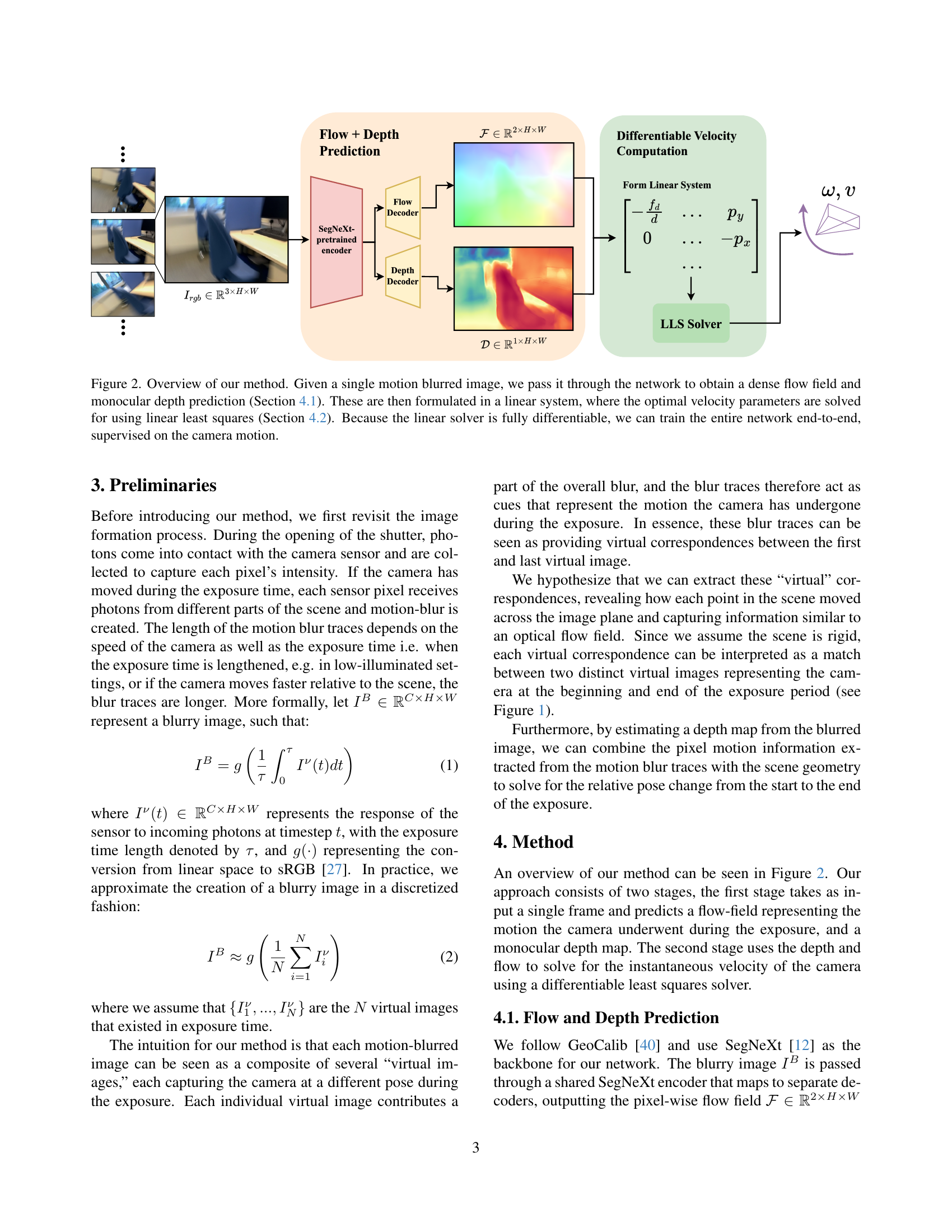
🔼 This figure illustrates the proposed method for estimating camera motion from a single motion-blurred image. The process begins by inputting a motion-blurred image into a neural network. This network predicts a dense flow field and a monocular depth map. These predictions are then used to construct a linear system of equations, solved using linear least squares to estimate the optimal camera velocity parameters. The method’s differentiability allows for end-to-end training of the entire network, directly supervised using known camera motion.
read the caption
Figure 2: Overview of our method. Given a single motion blurred image, we pass it through the network to obtain a dense flow field and monocular depth prediction (Section 4.1). These are then formulated in a linear system, where the optimal velocity parameters are solved for using linear least squares (Section 4.2). Because the linear solver is fully differentiable, we can train the entire network end-to-end, supervised on the camera motion.

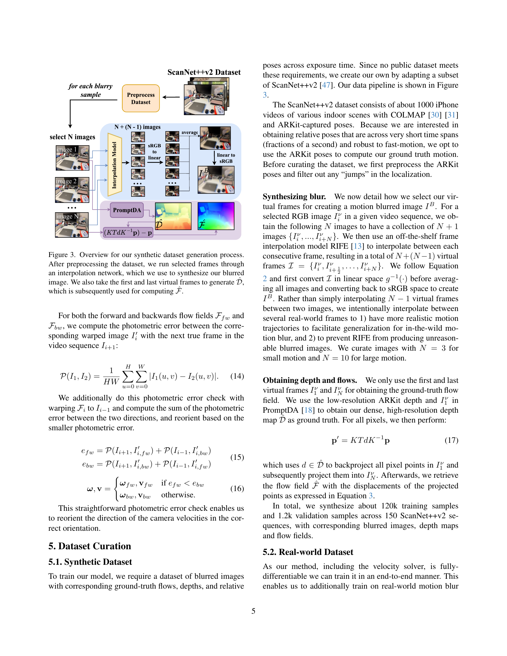
🔼 This figure illustrates the process of creating a synthetic dataset for training a model to estimate camera motion from a single motion-blurred image. The process begins with preprocessing a subset of the ScanNet++v2 dataset. Selected frames are then passed through an interpolation network (like RIFE) to generate a synthetic motion-blurred image. Simultaneously, the first and last frames from the sequence are used to create ground truth depth information (represented as \hat{D}). This depth map, along with the motion blurred image, is used to compute a ground truth dense flow field (represented as \hat{F}). These generated data points (blurred image, \hat{D}, and \hat{F}) comprise the synthetic training dataset.
read the caption
Figure 3: Overview for our synthetic dataset generation process. After preprocessing the dataset, we run selected frames through an interpolation network, which we use to synthesize our blurred image. We also take the first and last virtual frames to generate 𝒟^^𝒟\mathcal{\hat{D}}over^ start_ARG caligraphic_D end_ARG, which is subsequently used for computing ℱ^^ℱ\mathcal{\hat{F}}over^ start_ARG caligraphic_F end_ARG.

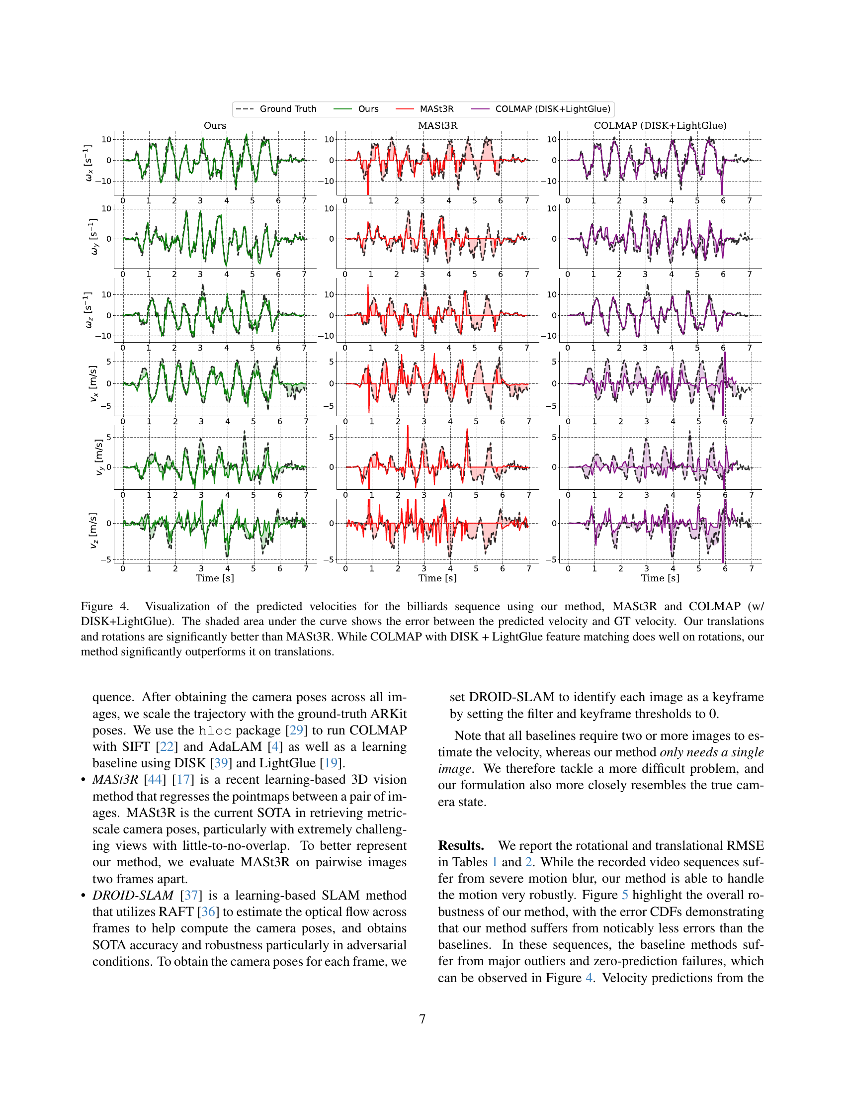
🔼 Figure 4 presents a comparison of the estimated velocities (rotational and translational) for the ‘billiards’ sequence obtained using three different methods: the proposed method, MASt3R, and COLMAP (combined with DISK and LightGlue). The shaded regions in the plots represent the error between each method’s velocity prediction and the ground truth velocity. The results demonstrate that the proposed method outperforms MASt3R in both rotational and translational velocity estimation. While COLMAP with DISK+LightGlue achieves comparable accuracy in rotational velocity estimation, the proposed method shows a clear advantage in translational velocity estimation.
read the caption
Figure 4: Visualization of the predicted velocities for the billiards sequence using our method, MASt3R and COLMAP (w/ DISK+LightGlue). The shaded area under the curve shows the error between the predicted velocity and GT velocity. Our translations and rotations are significantly better than MASt3R. While COLMAP with DISK + LightGlue feature matching does well on rotations, our method significantly outperforms it on translations.
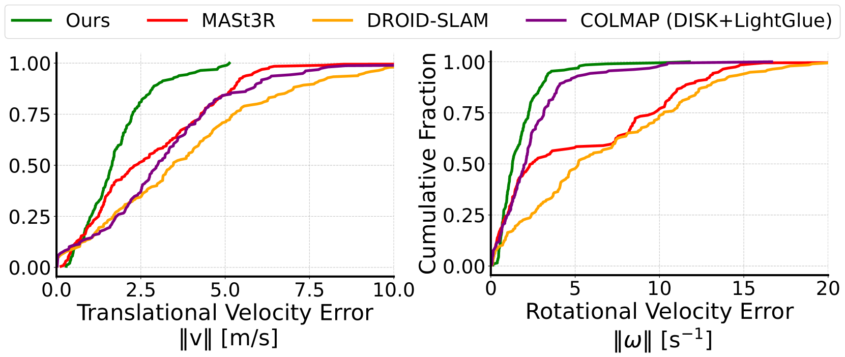
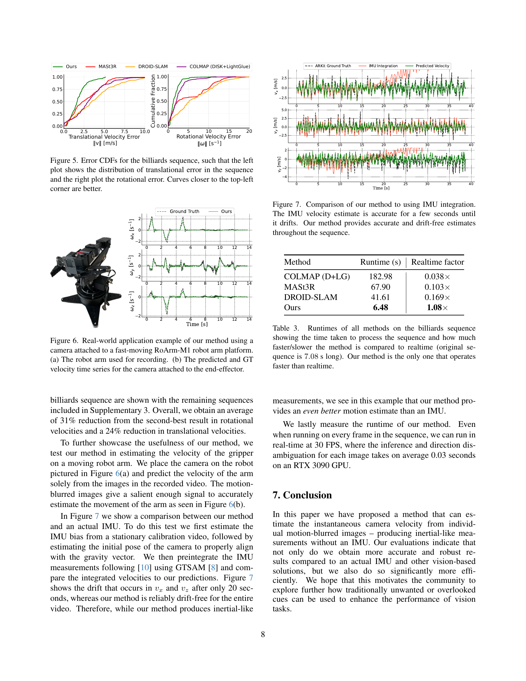
🔼 Figure 5 presents the cumulative distribution functions (CDFs) of the errors for translational and rotational velocities obtained from the billiards sequence. The left plot displays the CDF of the translational velocity errors, and the right plot shows the CDF of the rotational velocity errors. A curve closer to the top-left corner indicates better performance, meaning smaller errors in both translational and rotational velocity estimation. The closer the curve is to the top-left corner, the lower the errors are.
read the caption
Figure 5: Error CDFs for the billiards sequence, such that the left plot shows the distribution of translational error in the sequence and the right plot the rotational error. Curves closer to the top-left corner are better.

🔼 This figure showcases a real-world application of the proposed method. Panel (a) displays the robotic arm (RoArm-M1) used to capture the data. The arm’s rapid movement introduces significant motion blur into the captured images. Panel (b) presents a comparison of the velocity estimations. The graph plots the predicted camera velocity from the single motion-blurred images against the ground truth velocity obtained through IMU measurements and precise robotic arm pose estimations. This demonstrates the method’s effectiveness in accurately estimating camera motion from a single motion-blurred image, even during high-speed movements.
read the caption
Figure 6: Real-world application example of our method using a camera attached to a fast-moving RoArm-M1 robot arm platform. (a) The robot arm used for recording. (b) The predicted and GT velocity time series for the camera attached to the end-effector.

🔼 This figure compares the camera velocity estimates from the proposed method and IMU integration. The IMU initially provides accurate estimates, but it starts to drift after a few seconds. In contrast, the proposed method produces accurate and consistent velocity estimates throughout the entire sequence, highlighting its superior robustness and stability in handling long-duration camera motion.
read the caption
Figure 7: Comparison of our method to using IMU integration. The IMU velocity estimate is accurate for a few seconds until it drifts. Our method provides accurate and drift-free estimates throughout the sequence.
More on tables
| Method | billiards | commonroom | dining | office | avg | |
|---|---|---|---|---|---|---|
| / / | / / | / / | / / | / / | ||
| MI | COLMAP [30] [31] | |||||
| D+LG [39] [19] | 3.11 / 2.06 / 2.14 | 1.70 / 2.09 / 2.20 | 1.81 / 2.45 / 1.52 | |||
| MASt3R [44] [17] | 2.59 / 1.50 / 3.52 | 1.28 / 1.94 / 2.49 | 0.82 / 0.55 / 1.22 | 1.72 / 2.16 / 1.46 | 1.60 / 1.54 / 2.17 | |
| DROID-SLAM [37] | 3.28 / 2.00 / 2.65 | 2.23 / 1.47 / 1.25 | 1.44 / 0.65 / 0.91 | 1.98 / 2.40 / 1.23 | 2.23 / 1.63 / 1.51 | |
SI | Ours | 1.36 / 1.17 / 1.05 | 1.00 / 0.80 / 0.71 | 0.95 / 0.61 / 0.81 | 1.12 / 1.52 / 1.12 | 1.11 / 1.03 / 0.92 |
| Zero-Velocity baseline | 2.80 / 1.66 / 1.41 | 1.98 / 1.48 / 1.26 | 1.30 / 1.05 / 1.20 | 1.94 / 2.26 / 1.07 | 2.01 / 1.61 / 1.24 |
🔼 Table 2 presents a quantitative comparison of the Root Mean Squared Error (RMSE) for translational velocity estimations along the x, y, and z axes. The results are obtained from various visual odometry and SLAM methods applied to both multi-image and single-image scenarios. The RMSE values are expressed in meters per second (m/s). The table highlights the superior performance of the proposed method compared to several state-of-the-art baselines by bolding and underlining the best and second-best results. The ‘×’ symbol indicates that a particular method failed to reconstruct the camera poses for the given sequence.
read the caption
Table 2: RMSE for translational velocities across each axis, in m/s. We evaluate both multi-image (MI) and single-image (SI) methods. The best and second-best results are bolded and underlined, respectively. The ×\times× represents a failure to reconstruct the poses.
| Method | Runtime (s) | Realtime factor |
|---|---|---|
| COLMAP (D+LG) | 182.98 | 0.038 |
| MASt3R | 67.90 | 0.103 |
| DROID-SLAM | 41.61 | 0.169 |
| Ours | 6.48 | 1.08 |
🔼 This table presents the runtimes of different visual odometry and structure-from-motion methods on the ‘billiards’ video sequence. It compares the time each method took to process the 7.08-second video and shows the ratio of the processing time to real-time (7.08 seconds). The goal is to highlight the efficiency of each method, specifically noting that the proposed method is the only one capable of real-time operation.
read the caption
Table 3: Runtimes of all methods on the billiards sequence showing the time taken to process the sequence and how much faster/slower the method is compared to realtime (original sequence is 7.08 s7.08 s7.08\text{ s}7.08 s long). Our method is the only one that operates faster than realtime.
Full paper#
