TL;DR#
Large language models(LLMs) have revolutionized AI, but their computational demands are a bottleneck. Traditional runtime optimizations like quantization and pruning have limitations, urging complementary approaches to improve efficiency while maintaining simplicity and scaling. Addressing the challenge, the paper introduces novel way to enhance LLM efficiency.
The study presents FFN Fusion, an optimization technique that reduces sequential computation in LLMs by parallelizing Feed-Forward Network(FFN) layers. By identifying opportunities for parallelization, FFN Fusion transforms sequential operations into parallel ones, reducing inference latency while preserving model behavior. The authors introduce Ultra-253B-Base, derived from Llama-3.1-405B, demonstrating significant speedups and strong performance.
Key Takeaways#
Why does it matter?#
This paper introduces FFN Fusion, a groundbreaking technique for optimizing LLMs, and releases Ultra-253B-Base to the public. It paves the way for future research into parallel architectures and efficient AI, providing a valuable resource for researchers and practitioners.
Visual Insights#

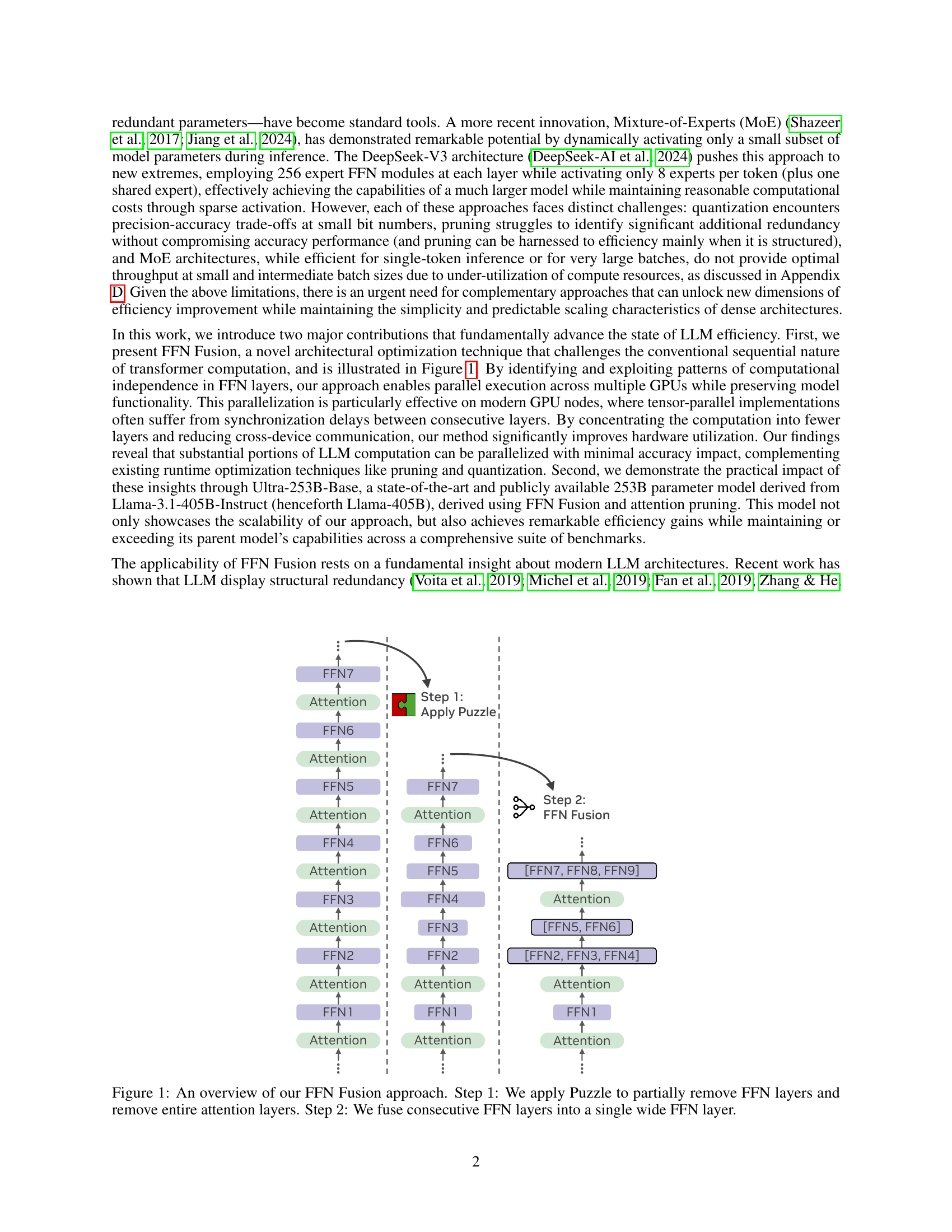
🔼 This figure illustrates the FFN Fusion technique used to optimize large language models. The process begins by using the Puzzle algorithm (Step 1) to remove some feed-forward network (FFN) layers and all attention layers from the model. The remaining FFN layers are often found in consecutive sequences. In Step 2, these sequences of FFN layers are ‘fused’ together into a single, wider FFN layer. This fusion allows for parallel processing of these layers, significantly increasing computational efficiency during inference without significantly impacting accuracy.
read the caption
Figure 1: An overview of our FFN Fusion approach. Step 1111: We apply Puzzle to partially remove FFN layers and remove entire attention layers. Step 2222: We fuse consecutive FFN layers into a single wide FFN layer.
| Model | Alignment | MMLU | MMLU-Pro | Arena Hard | HumanEval | MT-Bench |
|---|---|---|---|---|---|---|
| Ultra-253B-Base | ✗ | 85.17 | 71.11 | 71.81 | 84.14 | 9.10 |
| Ultra-253B-Base | ✓ | 85.13 | 72.25 | 84.92 | 86.58 | 9.19 |
🔼 This table presents a comparison of the Ultra-253B-Base model’s performance on several benchmark datasets before and after applying an alignment technique. The benchmarks assess the model’s capabilities in different areas, such as reasoning and question answering. The ‘Alignment’ column indicates whether the alignment technique was applied. The table shows the performance scores (accuracy percentages) for the model on each benchmark.
read the caption
Table 1: Ultra-253B-Base performance before and after alignment.
In-depth insights#
FFN Parallelism#
FFN Parallelism could revolutionize LLM efficiency. By identifying computationally independent FFN layers, specifically post-attention removal, and processing them in parallel, we minimize accuracy impact while drastically cutting inference latency. This stems from LLMs exhibiting surprisingly low inter-layer dependencies, enabling the fusion of sequential FFN layers into a single, wider one for parallel execution. This approach excels in modern GPU setups, where tensor-parallel implementations often stumble due to synchronization delays. By concentrating computation into fewer layers and streamlining cross-device communication, we significantly enhance hardware utilization. This strategy could challenge the conventional sequential nature of transformer computation, offering a pathway to harness greater computational power. The key lies in exploiting computational independence and reducing synchronization overhead, ultimately making larger language models more accessible and efficient.
Puzzle & Fusion#
The concept of ‘Puzzle & Fusion’ suggests a combined strategy for optimizing large language models (LLMs). ‘Puzzle’ likely refers to a method of identifying and dissecting the LLM architecture to pinpoint redundant or inefficient components, possibly through techniques like neural architecture search (NAS) or pruning. By analogy, it can mean understanding each and every part of the puzzle (network) and their interactions. Then, ‘Fusion’ implies consolidating or merging remaining components to streamline computation. This could involve techniques like layer fusion (e.g., FFN Fusion), where multiple sequential operations are combined into a single, more efficient operation, thereby removing computational overheads, which results in faster processing and reduced memory footprint. The ultimate aim is to improve inference speed and resource utilization without significantly sacrificing model accuracy. The effectiveness of this approach hinges on the ability to identify truly independent or weakly dependent components that can be safely fused without disrupting the model’s overall functionality.
Ultra-253B-Base#
The research centers around a model named Ultra-253B-Base, which represents a core contribution. It’s derived from Llama-3.1-405B through ‘FFN Fusion’ and ‘attention pruning’, indicating a strategy of optimizing an existing architecture. Key achievements include significant efficiency gains without sacrificing performance, potentially surpassing its predecessor. This optimized model’s public release further emphasizes the study’s practical impact. Performance metrics suggest the model attains state-of-the-art results on key benchmarks, showcasing the effectiveness of ‘FFN Fusion’. The model achieves significant speedup in inference latency and reduced per-token cost. It underscores a commitment to improving accessibility. The model involves reducing parameter count, and improving memory footprint in KV-cache memory.
LLM Redundancy#
LLM Redundancy is implicitly explored. The paper delves into structural redundancy, with attention heads being selectively removed without significant accuracy loss, suggesting some heads are less critical. This parallels the idea of redundant parameters or computations within the network. The core idea of FFN Fusion exploits computational independence, implying certain FFN layers perform similar or non-essential transformations, enabling parallelization without impacting the model’s overall behavior. This reveals another layer of redundancy, this time at the architectural level. Even entire blocks may be parallelizable, showing potential for further redundancy exploitation to improve efficiency.
MoE Tradeoffs#
Mixture-of-Experts (MoE) models present a unique set of tradeoffs compared to dense models. While they offer the potential for increased model capacity and performance with a seemingly manageable computational cost, several practical challenges limit their effectiveness. The routing mechanism in MoEs, while enabling conditional computation, itself introduces overhead. MoEs suffer from bad scaling with the number of tokens, larger low-level overheads, and worse parallelization scaling than dense models. The effectiveness of MoEs is highly dependent on batch size, load balancing, and hardware capabilities. Smaller batch sizes are not as efficient, while smaller layers incur large latency. Consequently, MoEs might not always be the optimal choice, especially when deployment constraints favor simplicity, predictable scaling, or smaller batch sizes. Dense models, enhanced with techniques like FFN Fusion, can offer a compelling alternative, providing a balance between performance and efficiency.
More visual insights#
More on figures

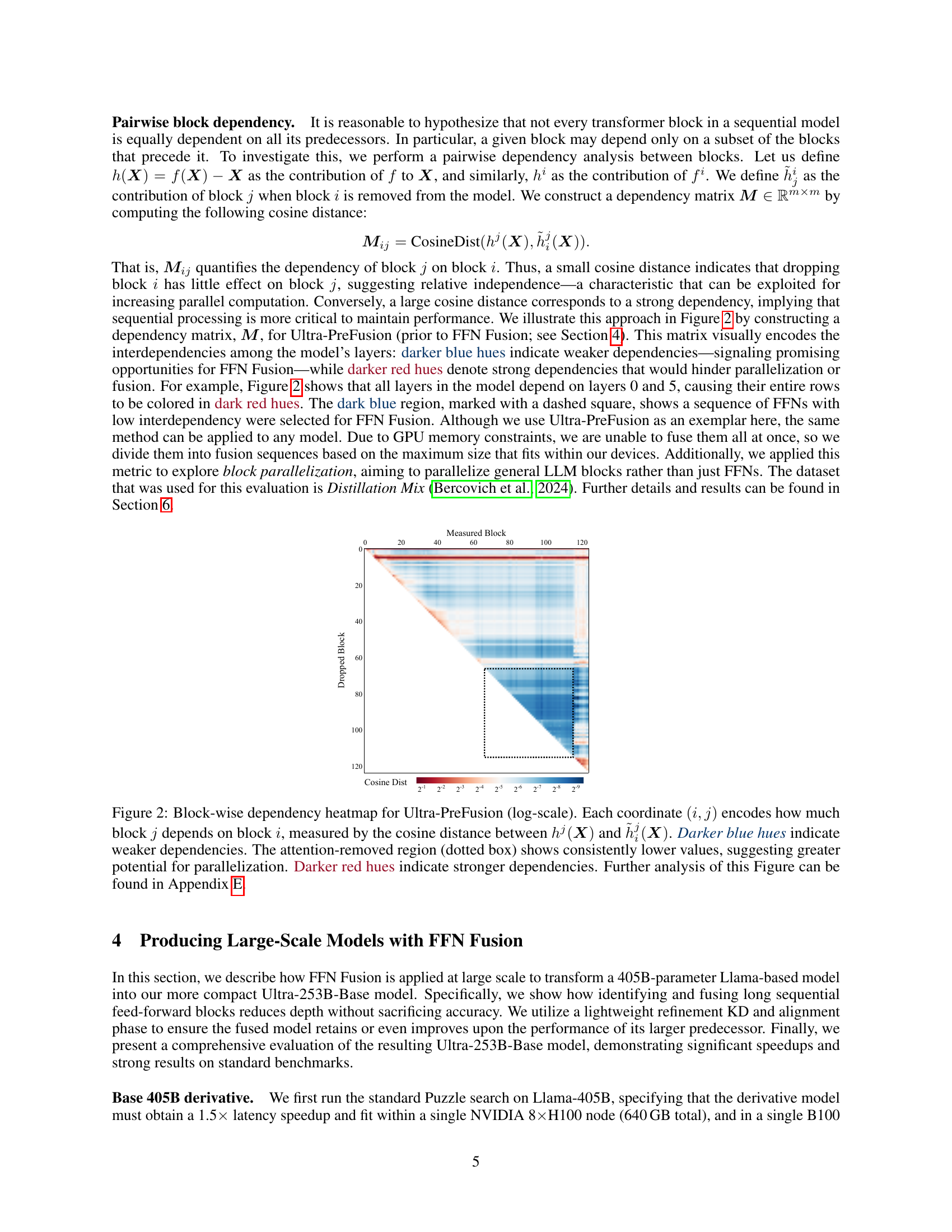
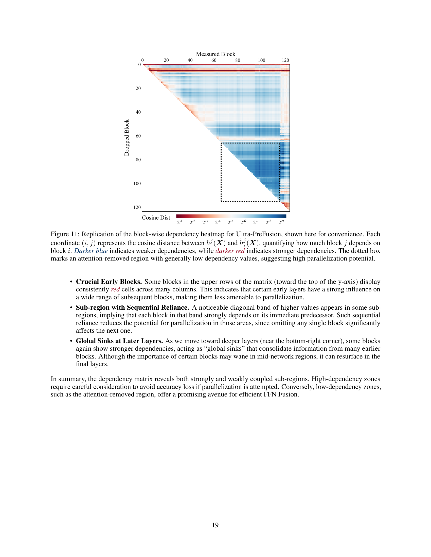
🔼 This figure is a heatmap visualizing the dependencies between blocks in the Ultra-PreFusion model. Each cell (i,j) represents the cosine similarity between the contribution of block j to the model’s output when block i is present and when block i is removed. Darker blue indicates low dependency (good for parallelization), and darker red indicates high dependency (bad for parallelization). The dotted box highlights a region where attention layers have been removed, showing low inter-block dependencies, thus indicating a good candidate for FFN fusion.
read the caption
Figure 2: Block-wise dependency heatmap for Ultra-PreFusion (log-scale). Each coordinate (i,j)𝑖𝑗(i,j)( italic_i , italic_j ) encodes how much block j𝑗jitalic_j depends on block i𝑖iitalic_i, measured by the cosine distance between hj(𝑿)superscriptℎ𝑗𝑿h^{j}({\bm{X}})italic_h start_POSTSUPERSCRIPT italic_j end_POSTSUPERSCRIPT ( bold_italic_X ) and h~ij(𝑿)subscriptsuperscript~ℎ𝑗𝑖𝑿\tilde{h}^{j}_{i}({\bm{X}})over~ start_ARG italic_h end_ARG start_POSTSUPERSCRIPT italic_j end_POSTSUPERSCRIPT start_POSTSUBSCRIPT italic_i end_POSTSUBSCRIPT ( bold_italic_X ). Darker blue hues indicate weaker dependencies. The attention-removed region (dotted box) shows consistently lower values, suggesting greater potential for parallelization. Darker red hues indicate stronger dependencies. Further analysis of this Figure can be found in Appendix E.

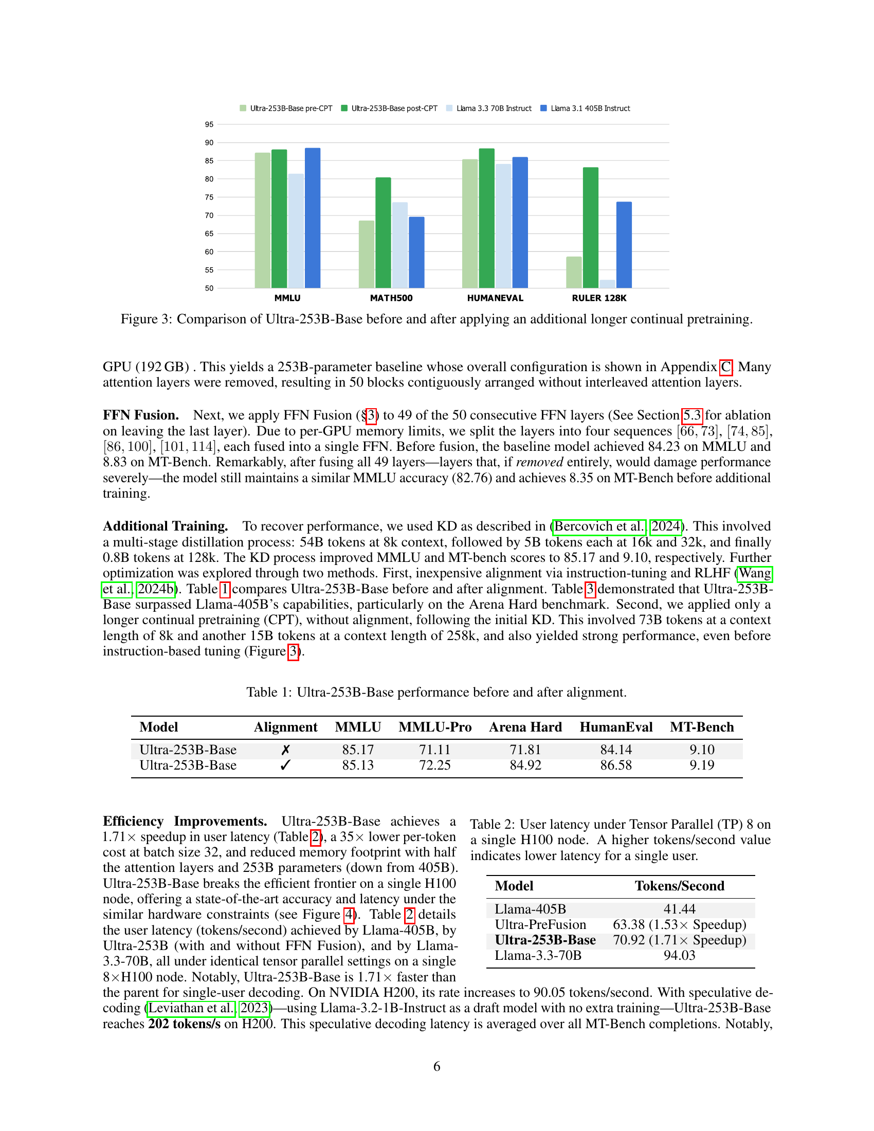
🔼 This figure compares the performance of the Ultra-253B-Base model before and after an additional, longer continual pre-training (CPT) phase. It shows benchmark results across several tasks (MMLU, MATH500, HumanEval, and RULER 128K) to illustrate the impact of the extended training on model accuracy. The bars represent the performance scores achieved on each benchmark for both the pre-CPT and post-CPT versions of the Ultra-253B-Base model, allowing for a direct visual comparison of improvements.
read the caption
Figure 3: Comparison of Ultra-253B-Base before and after applying an additional longer continual pretraining.

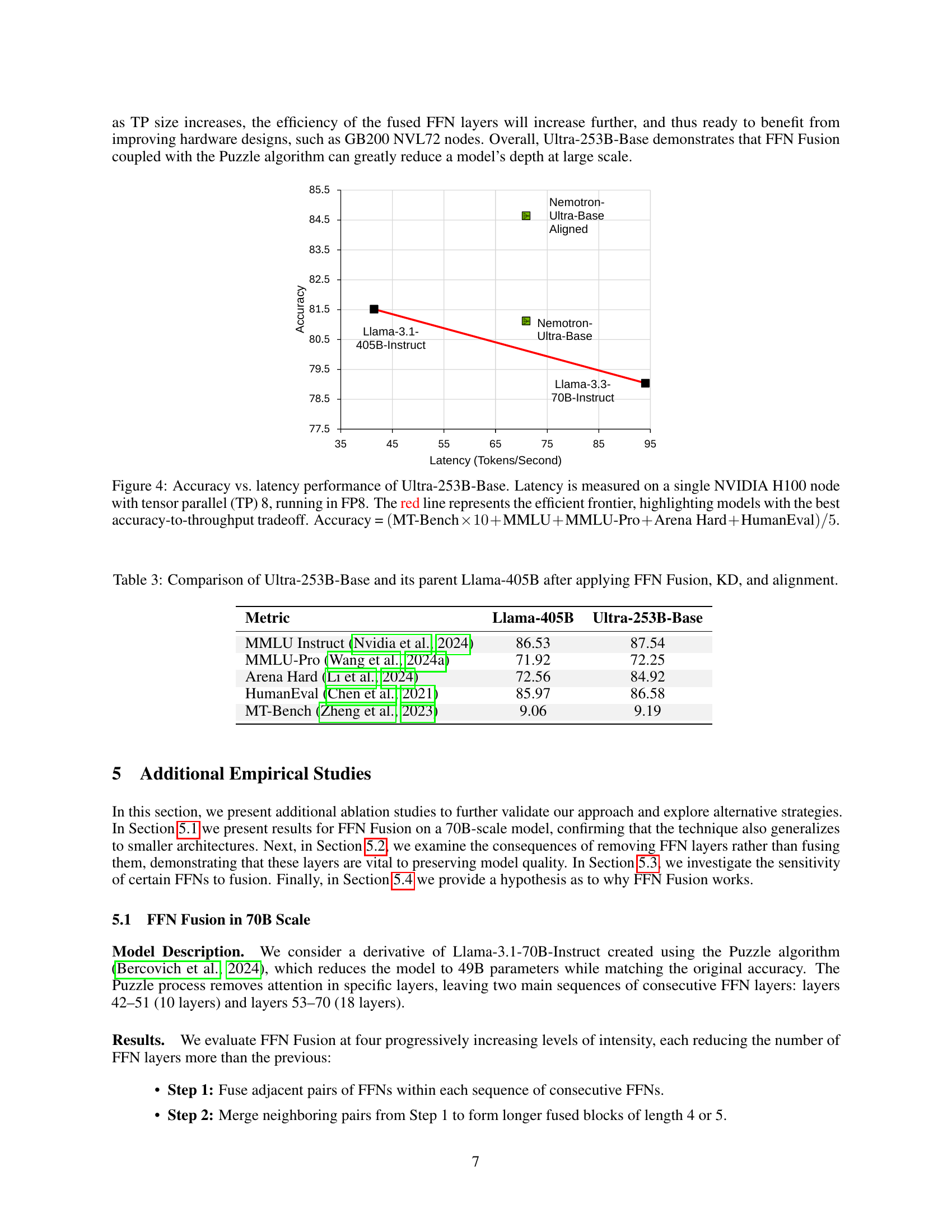
🔼 Figure 4 presents a performance comparison of the Ultra-253B-Base language model against other models. The x-axis represents the model’s inference latency (measured in tokens per second) on a single NVIDIA H100 GPU with tensor parallelism (TP8) using FP8 precision. The y-axis shows the model’s accuracy, which is a composite score calculated as the average of several benchmark metrics. The benchmarks include MT-Bench (weighted 10x), MMLU, MMLU-Pro, Arena Hard, and HumanEval. The red line illustrates the efficient frontier, which highlights the models that best balance accuracy and speed. Points above the red line represent models that achieve higher accuracy for a given latency, indicating superior performance.
read the caption
Figure 4: Accuracy vs. latency performance of Ultra-253B-Base. Latency is measured on a single NVIDIA H100 node with tensor parallel (TP) 8, running in FP8. The red line represents the efficient frontier, highlighting models with the best accuracy-to-throughput tradeoff. Accuracy = (MT-Bench×10+MMLU+MMLU-Pro+Arena Hard+HumanEval)/5MT-Bench10MMLUMMLU-ProArena HardHumanEval5(\text{MT-Bench}\times 10+\text{MMLU}+\text{MMLU-Pro}+\text{Arena Hard}+\text{% HumanEval})/5( MT-Bench × 10 + MMLU + MMLU-Pro + Arena Hard + HumanEval ) / 5.

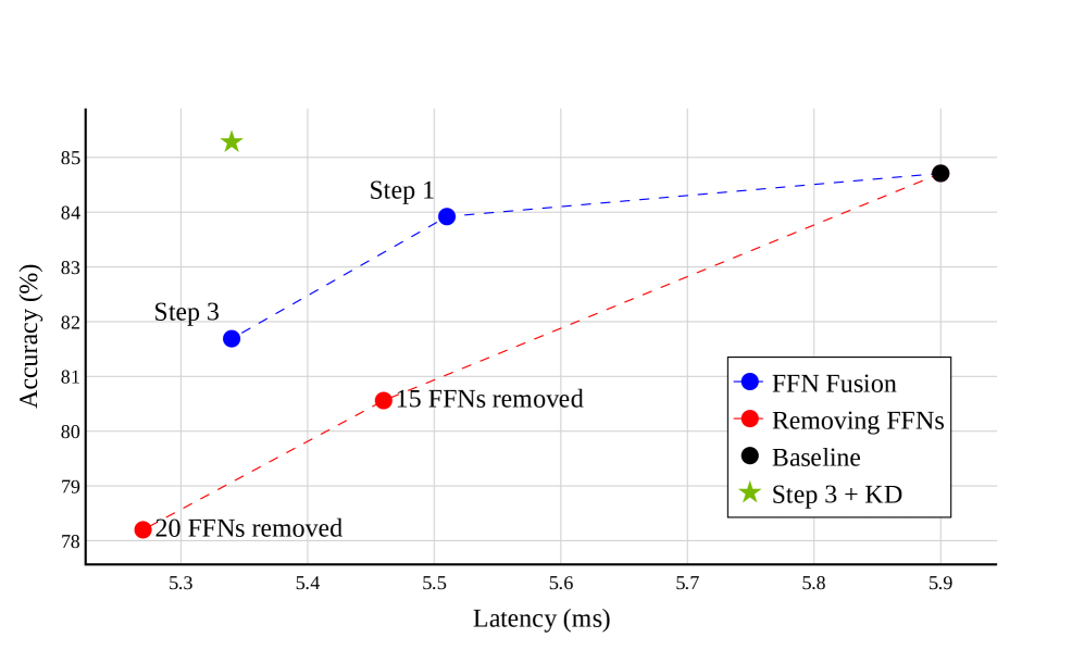
🔼 This figure compares the accuracy and latency trade-offs between removing FFN layers and fusing them using FFN Fusion. The x-axis represents latency (in milliseconds), and the y-axis represents accuracy (%). Multiple lines are shown, each representing a different strategy: (1) a baseline (no FFN removal or fusion), (2) removal of 15 FFN layers, (3) removal of 20 FFN layers, (4) applying FFN Fusion in a single step, and (5) applying FFN Fusion followed by knowledge distillation (KD). The results demonstrate that FFN Fusion achieves significantly better accuracy at comparable latencies compared to simply removing FFN layers. Knowledge distillation further improves the performance of the fusion method.
read the caption
Figure 5: Accuracy vs. Latency for FFN Removal vs. Fusion.
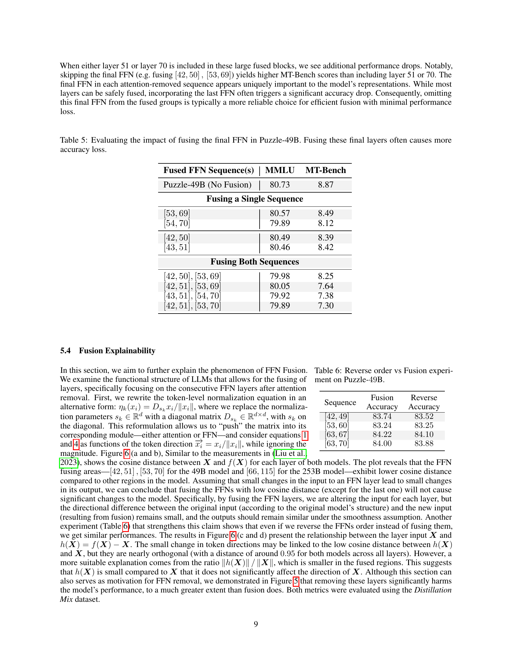
🔼 Figure 6 presents a per-layer analysis of two key metrics, comparing the 49B and 253B models. The top row shows the cosine distance between the input (X) and the output (f(X)) of each layer. A lower cosine distance suggests that the layer’s output is very similar to its input, implying less processing and transformation is occurring. The bottom row visualizes the ratio of h(X) (the block’s contribution to X) to X itself. A lower ratio indicates that the layer has minimal effect on the input’s direction, suggesting a low dependency on preceding layers. This analysis helps to identify regions within the model that are suitable for parallelization, as observed by minimal impact from fusing FFN layers.
read the caption
Figure 6: Per-layer metrics. Upper row is the cosine distance between f(𝑿)𝑓𝑿f({\bm{X}})italic_f ( bold_italic_X ) and 𝑿𝑿{\bm{X}}bold_italic_X for the (a) The 49B model and (b) Ultra-253B-Base model. Bottom row represents the ratio between h(𝑿)ℎ𝑿h({\bm{X}})italic_h ( bold_italic_X ) and 𝑿𝑿{\bm{X}}bold_italic_X for the (c) The 49B model and (d) Ultra-253B-Base model.

🔼 This figure shows the cosine distance between the output of each layer and its input for the 49B parameter model (left) and the Ultra-253B-Base model (right). The cosine distance is a measure of the similarity between two vectors; a lower cosine distance indicates higher similarity. The plot shows that in certain regions of the model (primarily those with fused FFN layers), the cosine distance between the input and output is relatively small. This suggests that the FFN layers in these regions have a limited effect on the input’s direction, allowing them to be fused without significantly impacting the model’s accuracy. The low cosine distance in these regions is a key observation supporting the FFN Fusion optimization technique.
read the caption
(a)

🔼 This figure shows the heatmap of the block-wise dependency for the Ultra-PreFusion model (before applying FFN fusion). The heatmap visualizes the dependency between blocks using cosine distance. Darker blue colors represent lower dependency (meaning blocks are relatively independent), while darker red colors indicate higher dependency (meaning blocks are strongly dependent). The figure highlights a region where multiple consecutive FFN layers exhibit low interdependencies, suggesting a significant potential for parallelization using FFN fusion. The dark blue region (marked by a dashed square) indicates such a region, while the redder regions indicate higher dependencies making parallelization more challenging or potentially less effective.
read the caption
(b)
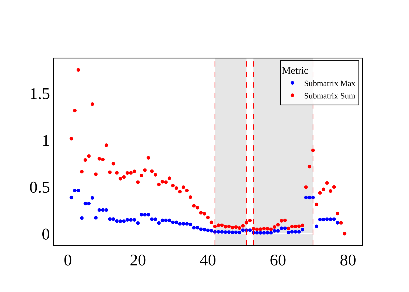
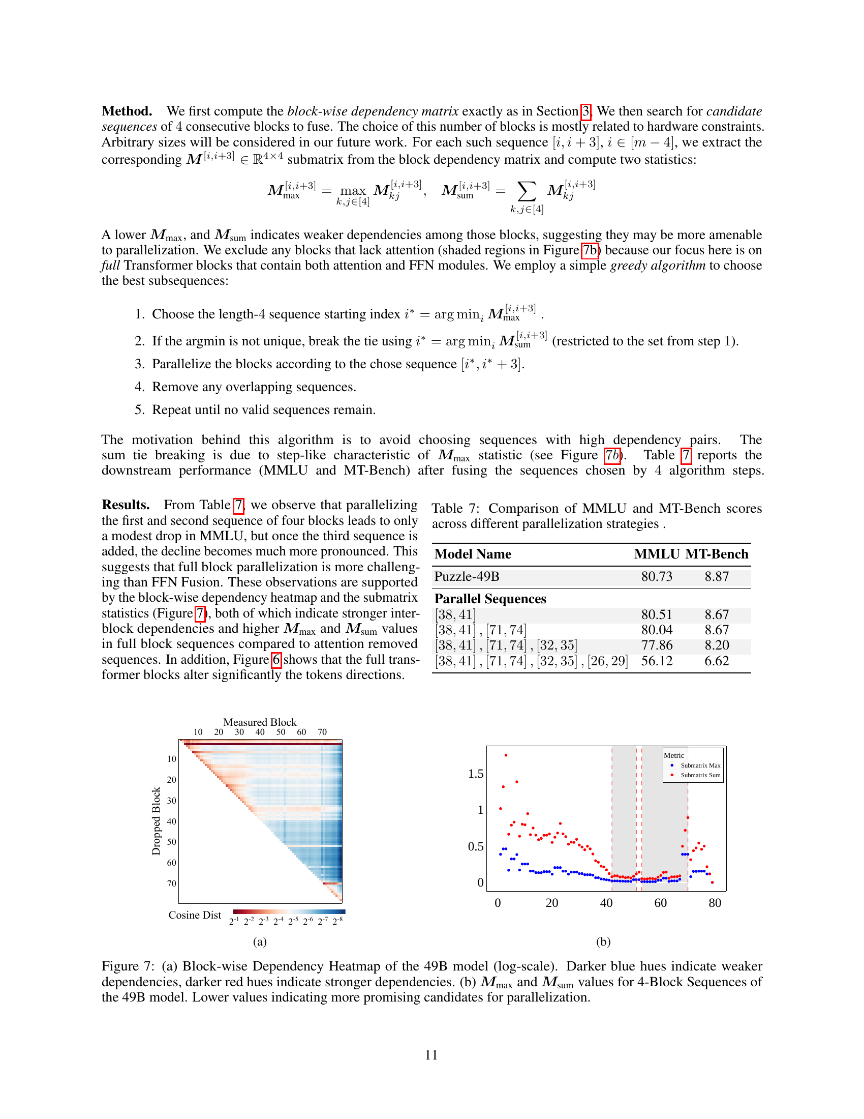
🔼 Figure 7 visualizes the dependencies between blocks in a 49B parameter language model. Panel (a) is a heatmap showing pairwise dependencies; darker blue indicates weaker dependence, while darker red shows stronger dependence. Panel (b) displays two metrics (Mmax and Msum) calculated for sequences of four consecutive blocks, which quantify the maximum and sum of dependencies within those sequences, respectively. Lower values of Mmax and Msum suggest greater potential for parallelization.
read the caption
Figure 7: (a) Block-wise Dependency Heatmap of the 49B model (log-scale). Darker blue hues indicate weaker dependencies, darker red hues indicate stronger dependencies. (b) 𝑴maxsubscript𝑴max{\bm{M}}_{\text{max}}bold_italic_M start_POSTSUBSCRIPT max end_POSTSUBSCRIPT and 𝑴sumsubscript𝑴sum{\bm{M}}_{\text{sum}}bold_italic_M start_POSTSUBSCRIPT sum end_POSTSUBSCRIPT values for 4-Block Sequences of the 49B model. Lower values indicating more promising candidates for parallelization.

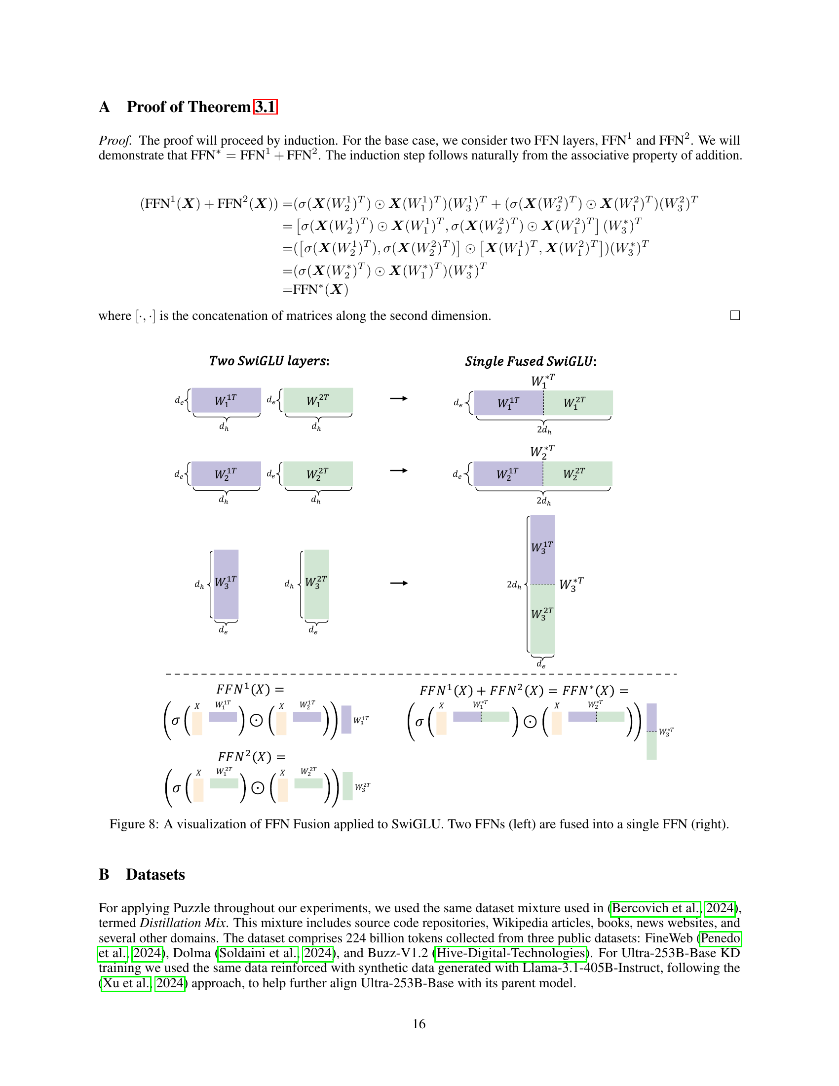
🔼 Figure 8 illustrates the FFN Fusion technique applied to the SwiGLU activation function. The left side shows two separate SwiGLU layers, each with its own weight matrices (W1, W2, W3). The input to the second layer depends on the output of the first. FFN Fusion combines these two layers into a single, wider SwiGLU layer (right). The new layer has combined weight matrices which achieve the same result as the two sequential layers but allows for parallel processing. The figure visually demonstrates the effect of reducing sequential computations and improving efficiency by merging FFN layers.
read the caption
Figure 8: A visualization of FFN Fusion applied to SwiGLU. Two FFNs (left) are fused into a single FFN (right).

🔼 This figure shows the layout of attention layers in the Ultra-PreFusion model before applying FFN Fusion. The x-axis represents the layer index, and the y-axis indicates the type of layer. The figure visually represents the sequence and distribution of attention layers and other layers within the model’s architecture. This helps to illustrate the pattern of attention layers that are removed or fused during model optimization.
read the caption
(a) Ultra-PreFusion Attention Layout

🔼 This figure shows the layout of feed-forward networks (FFNs) in the Ultra-PreFusion model. It illustrates the arrangement of FFN layers, their widths (number of neurons), and how they are distributed throughout the model’s architecture. The x-axis represents the layer index, and the y-axis represents the FFN width (or the number of neurons in each FFN layer). The plot visually depicts the changes in the width of the FFN layers across the various layers of the model. This visualization helps to understand the model’s structure and how the computational complexity varies across different layers.
read the caption
(b) Ultra-PreFusion FFN Layout

🔼 This figure is a visualization of the attention layers layout in the Puzzle-49B model architecture. It shows the arrangement and quantity of attention layers across the model’s layers, illustrating how the Puzzle algorithm has pruned or removed certain layers. The x-axis represents the layer index, while the y-axis shows the number of attention layers present at each layer. The figure helps in understanding the sparsity introduced by the Puzzle optimization technique, specifically in the context of the 49B parameter model.
read the caption
(c) Puzzle-49B Attention Layout

🔼 This figure is a visualization of the feed-forward network (FFN) layer layout for the Puzzle-49B model. It shows the number of FFN layers across the model’s depth, and visually depicts the varying widths of these FFN layers as a result of the Puzzle algorithm’s optimization. The x-axis represents the layer index and the y-axis represents the width (scaling multiplier) of the FFN layer. This helps illustrate the effect of Puzzle in making FFN layer widths vary across the layers, and highlights sequences of consecutive FFN layers resulting from the pruning of attention layers.
read the caption
(d) Puzzle-49B FFN Layout

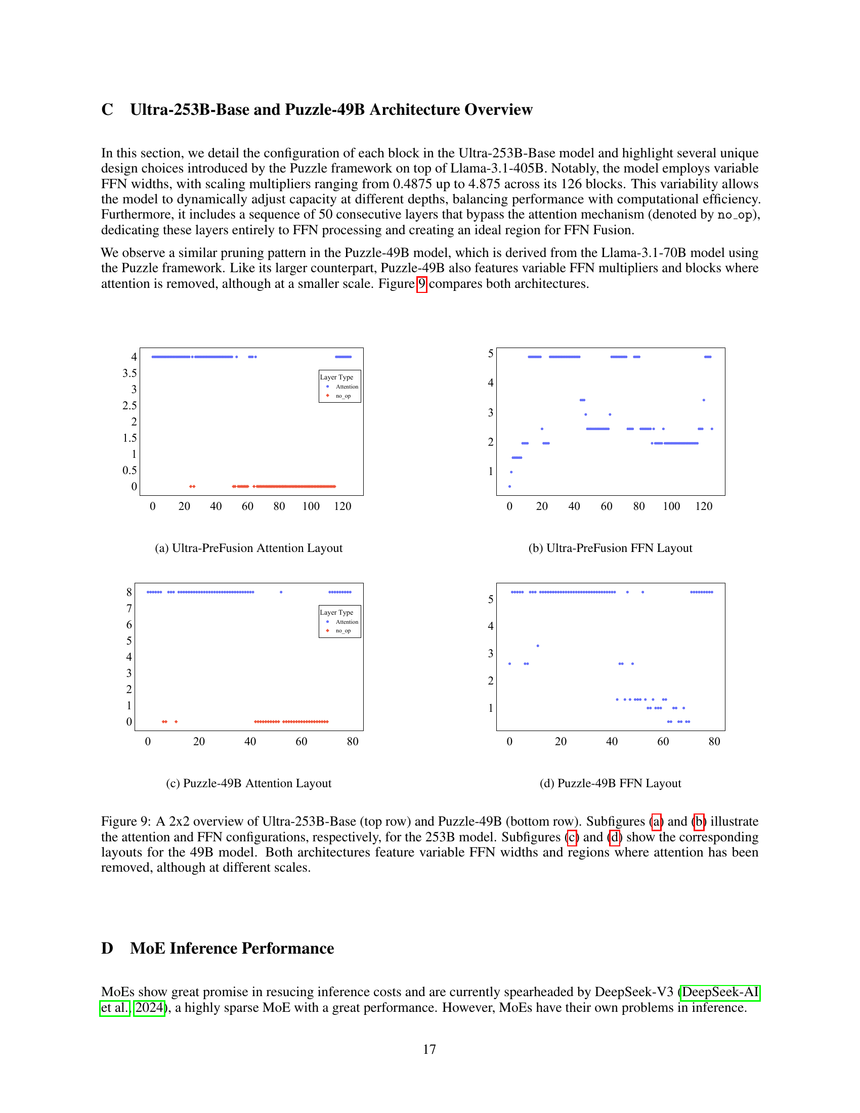
🔼 This figure provides a detailed comparison of the architectural layouts of two large language models: Ultra-253B-Base and Puzzle-49B. The top row displays the architecture of the Ultra-253B-Base model, showing the arrangement of attention and feed-forward network (FFN) layers. The bottom row shows the corresponding architecture for the Puzzle-49B model. Subfigures (a) and (b) specifically detail the attention and FFN layers, respectively, within the Ultra-253B-Base model. Subfigures (c) and (d) present the same information for the Puzzle-49B model. A key takeaway is that both models exhibit variable FFN widths and sections where attention layers have been removed, although the scale of these variations differs between the two models.
read the caption
Figure 9: A 2x2 overview of Ultra-253B-Base (top row) and Puzzle-49B (bottom row). Subfigures (9(a)) and (9(b)) illustrate the attention and FFN configurations, respectively, for the 253B model. Subfigures (9(c)) and (9(d)) show the corresponding layouts for the 49B model. Both architectures feature variable FFN widths and regions where attention has been removed, although at different scales.

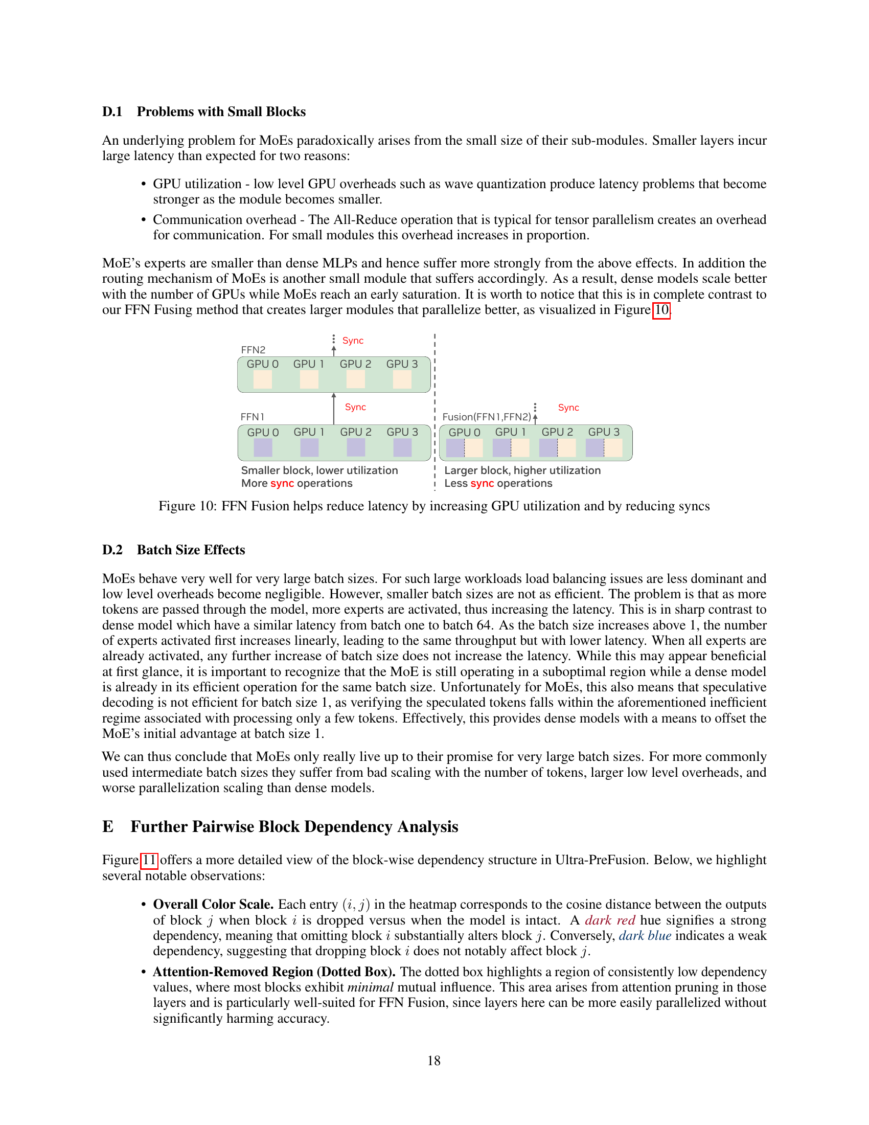
🔼 This figure illustrates how FFN Fusion improves latency. The left side shows a traditional approach with sequential FFN layers (FFN1 and FFN2). Each FFN layer requires synchronization (represented by the ‘Sync’ label), leading to longer execution times due to the need for communication between GPUs. In contrast, the right side depicts the FFN Fusion method, where FFN1 and FFN2 are merged into a single, wider layer. This reduces the number of synchronization points and increases GPU utilization, resulting in faster inference latency.
read the caption
Figure 10: FFN Fusion helps reduce latency by increasing GPU utilization and by reducing syncs
More on tables
| Model | Tokens/Second |
|---|---|
| Llama-405B | 41.44 |
| Ultra-PreFusion | 63.38 (1.53 Speedup) |
| Ultra-253B-Base | 70.92 (1.71 Speedup) |
| Llama-3.3-70B | 94.03 |
🔼 This table presents a comparison of the inference latency (measured as tokens per second) for different large language models (LLMs) running on a single NVIDIA H100 GPU with Tensor Parallelism set to 8. Lower latency is better, indicating faster inference. The models compared include Llama-405B (the original model), Ultra-PreFusion (an intermediate model produced through attention pruning), and Ultra-253B-Base (the final model obtained using FFN Fusion). The table also includes a 70B parameter model for comparison. The results showcase the speedup achieved by FFN Fusion, which helps optimize the model’s performance.
read the caption
Table 2: User latency under Tensor Parallel (TP) 8 on a single H100 node. A higher tokens/second value indicates lower latency for a single user.
| Metric | Llama-405B | Ultra-253B-Base |
|---|---|---|
| MMLU Instruct (Nvidia et al., 2024) | 86.53 | 87.54 |
| MMLU-Pro (Wang et al., 2024a) | 71.92 | 72.25 |
| Arena Hard (Li et al., 2024) | 72.56 | 84.92 |
| HumanEval (Chen et al., 2021) | 85.97 | 86.58 |
| MT-Bench (Zheng et al., 2023) | 9.06 | 9.19 |
🔼 This table presents a comparison of the performance of the Ultra-253B-Base model and its parent model, Llama-405B, across several key benchmarks. Ultra-253B-Base is derived from Llama-405B through the application of three optimization techniques: FFN Fusion (a novel parallelization technique), Knowledge Distillation (KD), and alignment. The table shows the accuracy scores achieved by both models on these benchmarks, highlighting the impact of the optimization techniques on model performance while maintaining or even surpassing the original model’s capabilities.
read the caption
Table 3: Comparison of Ultra-253B-Base and its parent Llama-405B after applying FFN Fusion, KD, and alignment.
| Model | Fusion | MMLU | MT-Bench | Accuracy |
|---|---|---|---|---|
| Baseline (49B Model) | - | |||
| Step 1 | ||||
| Step 2 | ||||
| Step 3 | ||||
| Step 4 | ||||
| Step 3 + KD |
🔼 Table 4 presents the results of applying FFN Fusion to a 49B parameter model derived from Llama-3.1-70B-Instruct. The model was preprocessed using the Puzzle algorithm, resulting in two main sequences of consecutive FFN layers. FFN Fusion was applied in four steps of increasing intensity, each step reducing the number of FFN layers more than the previous. Each row shows the performance of a different fusion variant (MMLU accuracy, MT-Bench score, and a combined accuracy score). The second column displays how many original FFN layers were replaced by the fused layers in each step. The table demonstrates the trade-off between model efficiency (fewer layers) and accuracy as more aggressive fusion is applied.
read the caption
Table 4: Evaluation of FFN Fusion. A detailed description of each fusion step (step x𝑥xitalic_x) is provided in the main text. The second column from the left indicates how many FFN layers were replaced by the corresponding number of new layers.
| Fused FFN Sequence(s) | MMLU | MT-Bench |
|---|---|---|
| Puzzle-49B (No Fusion) | 80.73 | 8.87 |
| Fusing a Single Sequence | ||
| 80.57 | 8.49 | |
| 79.89 | 8.12 | |
| 80.49 | 8.39 | |
| 80.46 | 8.42 | |
| Fusing Both Sequences | ||
| 79.98 | 8.25 | |
| 80.05 | 7.64 | |
| 79.92 | 7.38 | |
| 79.89 | 7.30 | |
🔼 This table investigates the effects of including or excluding the last feed-forward network (FFN) layer when applying FFN fusion in the Puzzle-49B model. The table compares the model’s performance on the MMLU and MT-Bench benchmarks under various FFN fusion configurations. Different fusion strategies are tested, each involving different combinations of fusing FFN sequences in the model, with a particular focus on whether the final FFN in each sequence is included. The results illustrate the sensitivity of model accuracy to the inclusion or exclusion of these final FFN layers, demonstrating that omitting the last FFN often minimizes accuracy loss, while including it can result in substantial performance degradation.
read the caption
Table 5: Evaluating the impact of fusing the final FFN in Puzzle-49B. Fusing these final layers often causes more accuracy loss.
| Sequence |
|
| ||||
|---|---|---|---|---|---|---|
🔼 This table presents an ablation study comparing the performance of FFN Fusion against a reverse-order arrangement of FFN layers within the Puzzle-49B model. It shows the MMLU and MT-Bench accuracy scores for different configurations, illustrating the impact of fusing consecutive FFN layers versus simply reversing their order.
read the caption
Table 6: Reverse order vs Fusion experiment on Puzzle-49494949B.
| Fusion |
| Accuracy |
🔼 This table presents the results of an experiment evaluating different parallelization strategies on a 49B parameter language model. The strategies involve fusing varying numbers of consecutive transformer blocks for parallel processing, which is a departure from the standard sequential computation approach. The table shows the MMLU and MT-Bench scores achieved by the model under these different parallelization schemes, allowing for a comparison of accuracy trade-offs against the potential gains in speed offered by parallel execution. The baseline performance (no parallelization) is also included for reference.
read the caption
Table 7: Comparison of MMLU and MT-Bench scores across different parallelization strategies .
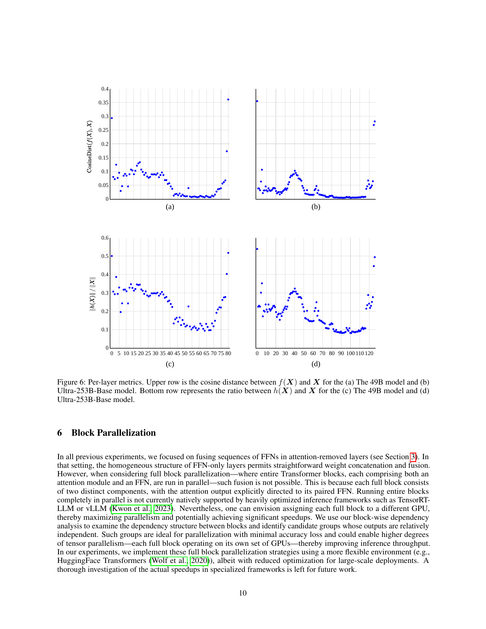
Full paper#