TL;DR#
Modern generative models break down complex image learning into simpler subtasks, but inherent conflicts arise during joint optimization. Existing solutions compromise efficiency or scalability. The core issue lies in how task decomposition affects synergies/conflicts between subtasks, motivating a principled framework that inherently aligns optimization targets across subtasks.
This paper presents an equivariant image modeling paradigm that minimizes inter-task conflicts. It uses column-wise tokenization to enhance translational symmetry and windowed causal attention for consistent contextual relationships. Experiments on ImageNet show performance comparable to state-of-the-art models with fewer resources. Analysis shows improved zero-shot generalization and ultra-long image synthesis.
Key Takeaways#
Why does it matter?#
This research introduces a novel equivariant image modeling framework, offering a pathway to efficient, conflict-free generative modeling. It’s highly relevant to current trends in generative AI and opens doors for new research into task-aligned decomposition and ultra-long image synthesis.
Visual Insights#

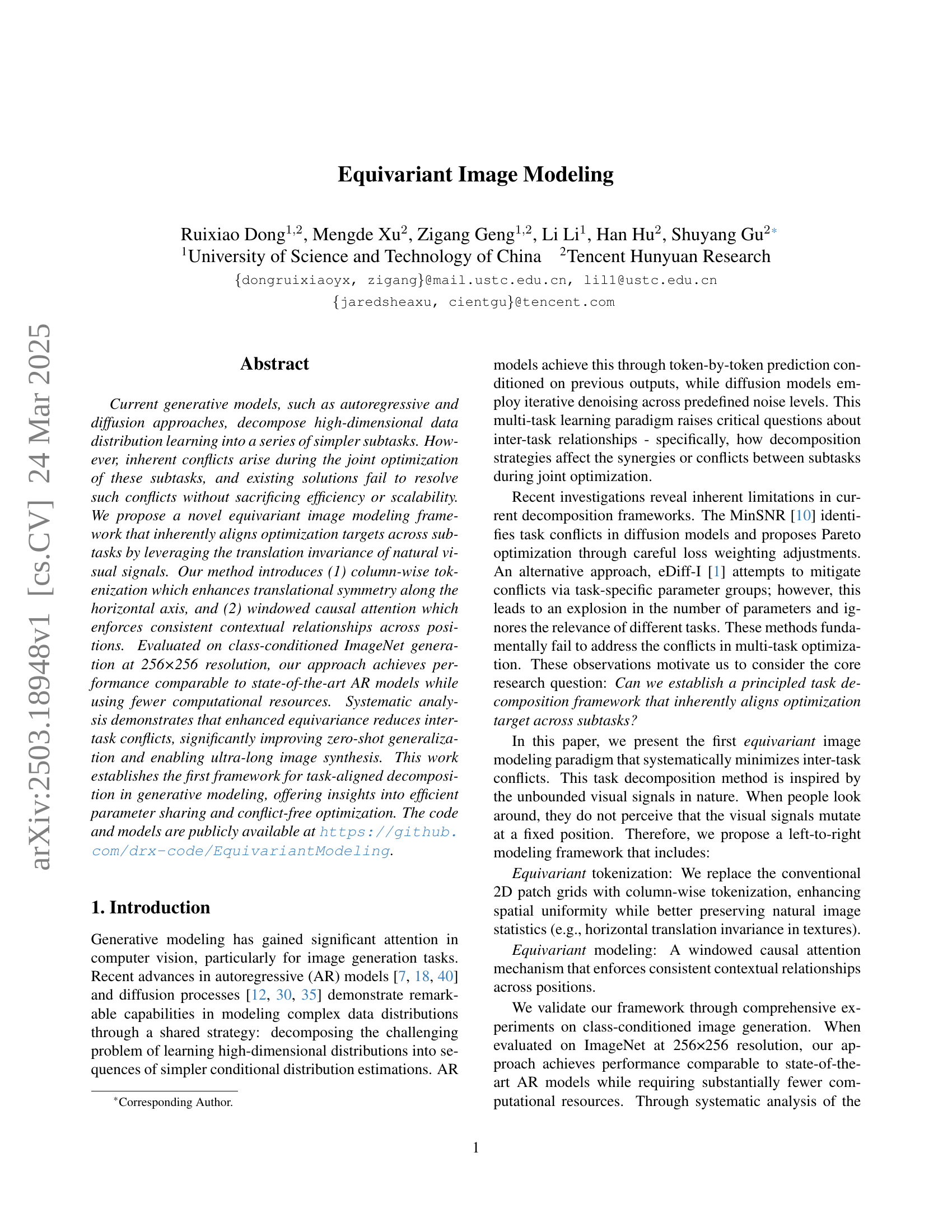
🔼 This figure illustrates the Equivariant Image Generation Framework, which consists of two main stages: tokenization and modeling. In the tokenization stage, a 1D tokenizer processes the input image, converting it into a sequence of 1D tokens arranged in columns. This is different from traditional methods that use 2D patches. Each token represents a vertical slice of image features. The modeling stage uses an enhanced autoregressive model to capture the relationships between these column-wise tokens, thereby predicting the image. This novel approach leverages the translational invariance of natural images, aligning optimization targets across sub-tasks to improve generation quality and efficiency.
read the caption
Figure 1: Illustration of Equivariant Image Generation Framework. The tokenizer translates the image into 1D tokens arranged in columns and an enhanced autoregressive model models the column-wise token distribution.
| Method | # Num task. | gFID |
|---|---|---|
| AR-MAR-2D | 16 | 7.93 |
| Ours | 16 | 5.57 |
| AR-MAR-2D | 8 | 92.46 |
| Ours | 8 | 8.99 |
🔼 This table presents the results of a zero-shot learning experiment. Models were trained on a subset of 16 subtasks and then evaluated on all 16 subtasks. The table compares the performance of the proposed method against a baseline method, measuring performance using the gFID (Generative Fréchet Inception Distance) metric. The number of training subtasks (# Num task.) is shown for both methods, highlighting the zero-shot generalization capabilities of the proposed approach.
read the caption
Table 1: Performance under Zero-shot Setting. # Num task. is used to denote the number of trained subtasks. The total number of subtasks is 16 for all methods.
In-depth insights#
Equivariance First#
Equivariance first is a compelling principle for generative modeling, particularly in domains like image generation where inherent symmetries exist. Prioritizing equivariance means designing models that explicitly respect these symmetries (e.g., translation, rotation). This can be achieved through architectural choices or training strategies that ensure consistent behavior under symmetry transformations. This approach offers several advantages. First, it improves sample efficiency: by leveraging symmetry, the model learns more generalizable representations from less data. Second, it enhances robustness: equivariant models are less susceptible to adversarial attacks or variations in input data. Third, it promotes interpretability: the model’s behavior becomes more predictable and easier to understand. It inherently reduces inter-task conflict as the optimization direction for perdicting any pixel remains consistent. The challenge lies in effectively incorporating equivariance without sacrificing model capacity or introducing unwanted biases. Carefully selecting appropriate architectural constraints and regularization techniques is crucial for realizing the full potential of an equivariance-first approach.
Column-wise Tokens#
Column-wise tokenization represents a departure from traditional 2D patch-based approaches in image modeling. By organizing image features into vertical columns, it enhances spatial uniformity and better preserves natural image statistics. This approach leverages the translation invariance of natural visual signals, addressing inherent conflicts arising during the joint optimization of subtasks in generative models. Column-wise tokenization facilitates more efficient parameter sharing across spatial locations, enabling the model to capture consistent contextual relationships and improve generalization capabilities. By eliminating the grid structure, this tokenization method provides a semantically continuous transition between tokens, creating a more equivariant representation conducive to autoregressive modeling.
Windowed Attention#
Windowed attention mechanisms offer a compelling approach to balancing computational efficiency and performance in sequence modeling. By limiting the scope of attention to a fixed-size window, the computational cost associated with attending to all previous tokens can be significantly reduced. This becomes particularly relevant in tasks dealing with long sequences, such as image generation where computational resources can be a bottleneck. However, this benefit comes with a trade-off: the model’s ability to capture long-range dependencies might be compromised. It is important to see how the window size impacts the ability to capture long-range dependencies. Further analysis may be warranted to determine the optimal window size that maximizes performance while remaining computationally feasible. There may be performance improvement by dynamically adapting window size with the aid of architectural re-design.
Zero-Shot Insight#
Zero-shot learning represents a significant leap in model generalization. The ability of a model to perform tasks it hasn’t been explicitly trained on is crucial for real-world applications where data scarcity is a common challenge. Insights from zero-shot performance can reveal the robustness and adaptability of the underlying feature representations. A strong zero-shot capability often indicates that the model has learned meaningful, transferable features rather than simply memorizing training data. The success in zero-shot scenarios hinges on effectively leveraging prior knowledge or learning from related tasks. This requires careful design of the model architecture and training strategies to ensure that the learned representations capture the essential characteristics of the data. The analysis of failures in zero-shot learning is equally important, providing valuable feedback on the limitations of the model and guiding future research directions.
Long Image Future#
The paper demonstrates a strong generalization ability across different subtasks, showcasing the power of equivariance. Inspired by unbounded visual signals, the model combines generalization to generate training-unseen subtasks with equivariant properties, testing models in long image generation scenarios. Trained on the Nature subset of Places, with 30 categories, the model generates extended-length, arbitrary-resolution images. These exhibit high spatial resolution and lengths significantly exceeding 256 pixels. The zero-shot long-content capability stems from inherent equivariance. Despite being optimized on 256x256 images, the model generates content at previously unencountered positional indices. Images up to eight times longer than the training inputs are produced, maintaining visual fidelity and avoiding sharp edges between generated regions. The method’s equivariance enables the generation of coherent, high-resolution long images without specific training for such scenarios.
More visual insights#
More on figures

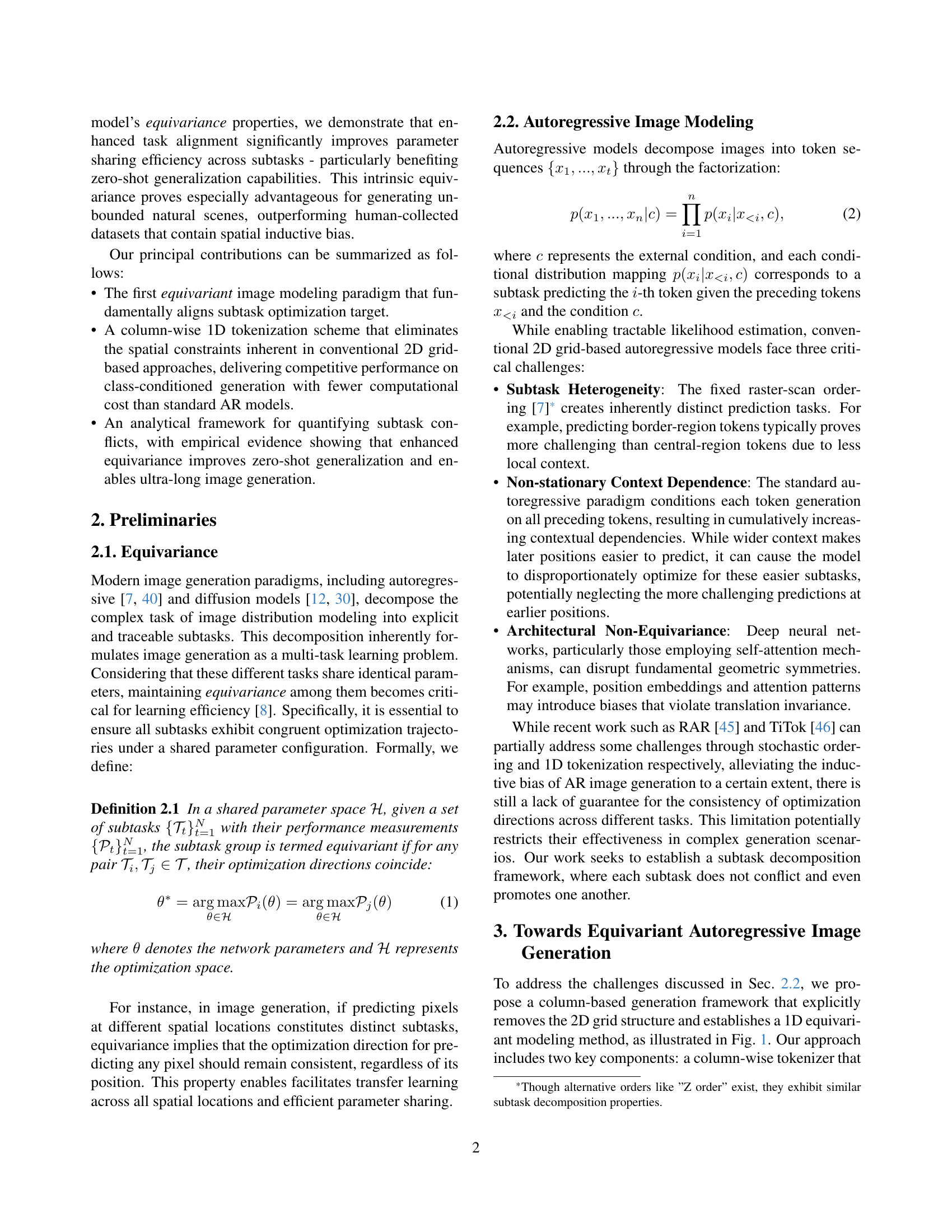
🔼 This figure demonstrates the process of reconstructing an image from 1D token sequences. Starting with a sequence of randomly initialized tokens, the model progressively replaces them with tokens encoded from the ground truth image. Each step in this replacement process results in a progressively more accurate reconstruction of the original image, visually showcasing how the tokens carry information that contributes to the reconstruction. The figure visually shows how the model successfully recovers the image, confirming the effectiveness of the proposed column-wise tokenization and the overall image generation process. It highlights that each token encodes a relevant part of the image, and together they represent the whole image.
read the caption
Figure 2: Visual Meanings of 1D Tokens. By progressively replacing the randomly initialized token sequence with tokens encoded from the ground truth images, the decoder faithfully reconstructs the original images step by step.

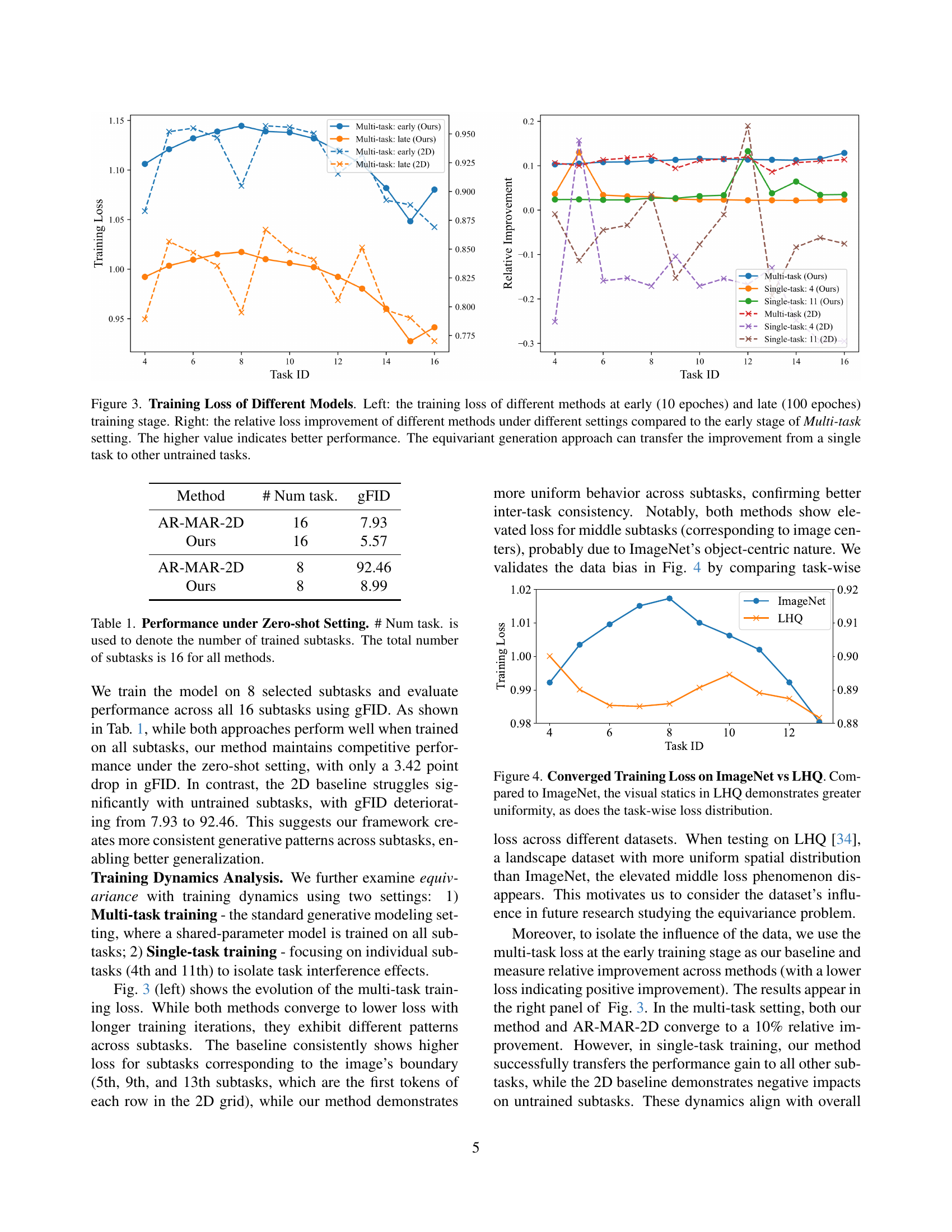
🔼 This figure displays the training loss curves for different image generation models. The left panel shows the absolute training loss at an early stage (10 epochs) and a later stage (100 epochs) of training. The right panel displays the relative improvement in training loss at the later stage compared to the loss at the early stage. Multiple training scenarios are included, such as the multi-task setting (training on all tasks), and single-task settings (training on only selected tasks). The comparison highlights how the proposed equivariant generation model achieves better parameter sharing and generalization, leading to consistent performance improvements across subtasks, unlike traditional 2D models where performance improvements in some tasks don’t transfer to others.
read the caption
Figure 3: Training Loss of Different Models. Left: the training loss of different methods at early (10 epoches) and late (100 epoches) training stage. Right: the relative loss improvement of different methods under different settings compared to the early stage of Multi-task setting. The higher value indicates better performance. The equivariant generation approach can transfer the improvement from a single task to other untrained tasks.

🔼 Figure 4 compares the converged training loss for different subtasks in the ImageNet and LHQ datasets. The ImageNet dataset shows a significant difference in the difficulty of different subtasks, with some subtasks consistently exhibiting higher loss than others. This uneven distribution across subtasks is likely due to the inherent bias in the ImageNet dataset towards objects that are centrally located and well-defined. In contrast, the LHQ dataset shows a much more uniform loss distribution across all subtasks, likely due to its higher degree of spatial uniformity. The figure suggests that the inconsistencies in the ImageNet data significantly impact the model’s training process.
read the caption
Figure 4: Converged Training Loss on ImageNet vs LHQ. Compared to ImageNet, the visual statics in LHQ demonstrates greater uniformity, as does the task-wise loss distribution.

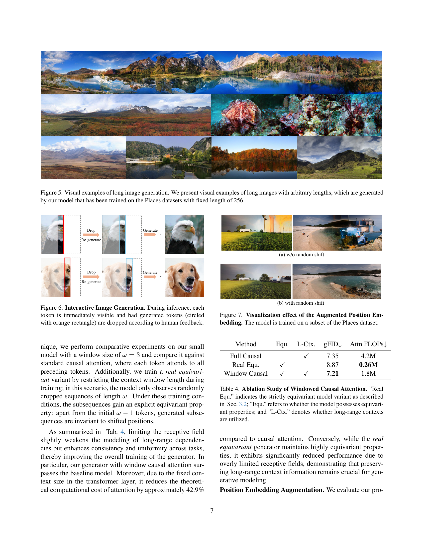
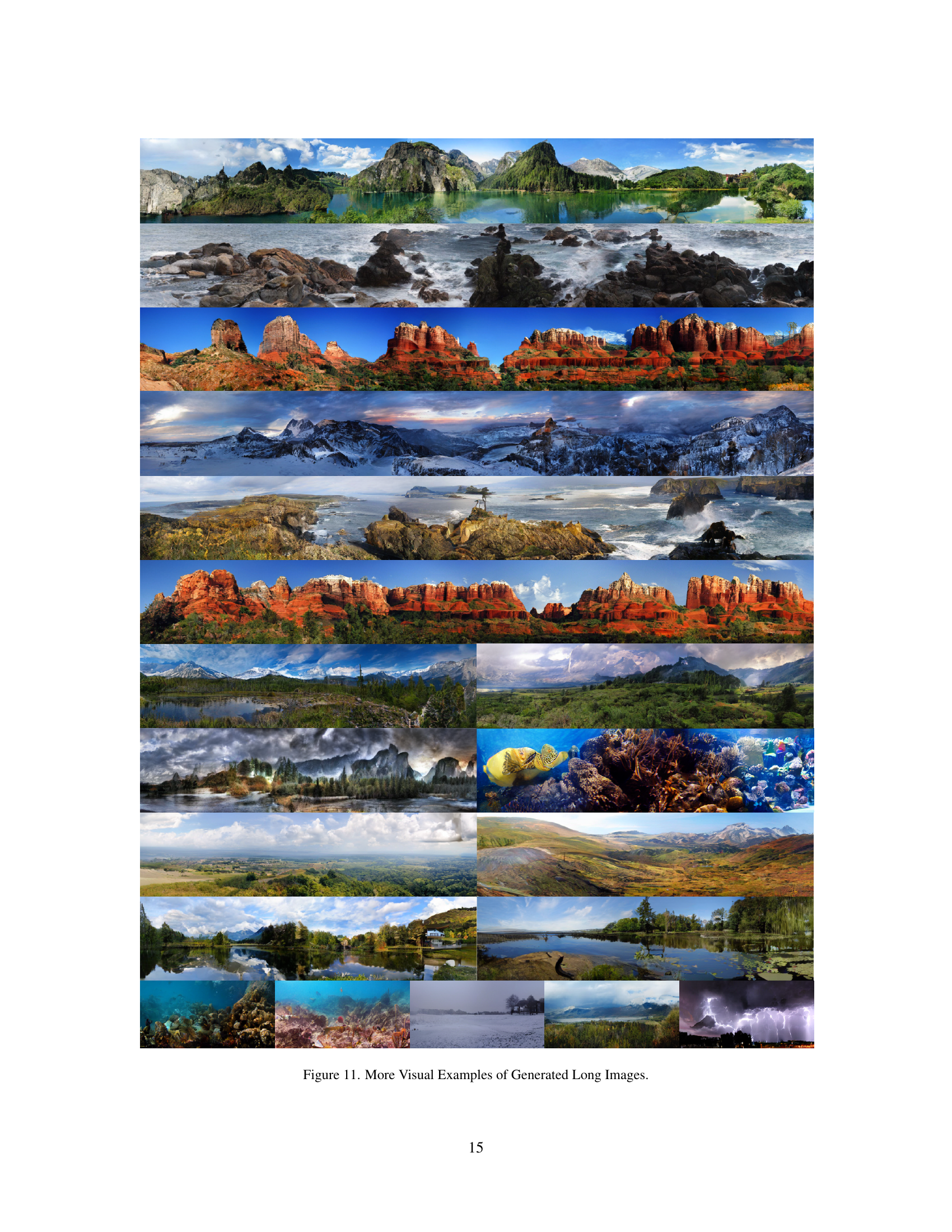
🔼 This figure showcases the model’s ability to generate images significantly longer than those it was trained on. The model was trained using images of a fixed 256-pixel length from the Places dataset. Despite this, the generated examples demonstrate the ability to produce images of arbitrary lengths, maintaining visual coherence and detail across the extended spatial range. This highlights the model’s generalization capability and robustness.
read the caption
Figure 5: Visual examples of long image generation. We present visual examples of long images with arbitrary lengths, which are generated by our model that has been trained on the Places datasets with fixed length of 256.

🔼 This figure demonstrates the interactive nature of the image generation process. Each token, representing a vertical strip of the image, is generated and displayed individually. The user can then review the generated image and identify any unsatisfactory tokens (highlighted in orange rectangles). These problematic tokens are then discarded, and the model regenerates them, allowing for human-guided refinement of the output image. This process iterates until the user is satisfied with the generated image.
read the caption
Figure 6: Interactive Image Generation. During inference, each token is immediately visible and bad generated tokens (circled with orange rectangle) are dropped according to human feedback.

🔼 This figure is a visualization showing the effect of augmented position embedding on image generation. The ‘(a) w/o random shift’ indicates that this specific image was generated without applying random shifts to the position indices during training. This augmentation helps the model better learn consistent relationships across different spatial locations, improving the quality and coherence of generated images, especially those that extend beyond the length of sequences seen during training.
read the caption
(a) w/o random shift

🔼 This figure visualizes the impact of the augmented position embedding technique on the model’s ability to generate coherent and continuous images. The left panel (a) shows results without random position shifts, while the right panel (b) demonstrates the results with random position shifts applied. The use of random position shifts helps to reduce the effect of fixed positions in the model and enhances its generation performance, especially for longer image sequences.
read the caption
(b) with random shift

🔼 This figure compares the results of using a standard positional embedding technique versus an augmented positional embedding technique in a transformer-based image generation model. The model was trained on a subset of the Places dataset. The augmented approach enhances the model’s ability to generate images with consistent visual features across spatial positions.
read the caption
Figure 7: Visualization effect of the Augmented Position Embedding. The model is trained on a subset of the Places dataset.

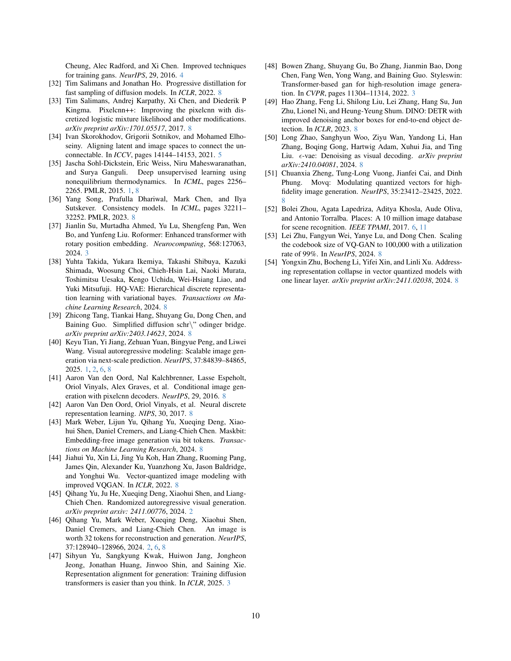
🔼 This figure provides additional examples to illustrate how the column-wise tokenization approach preserves the vertical equivariance of natural images. Each image shows the progressive reconstruction of an image from its 1D token representation. The reconstruction starts with a randomly initialized sequence of tokens and progressively replaces those random tokens with tokens generated from the ground truth image. This demonstrates how the model reconstructs the image from a column-wise representation, highlighting the effectiveness of the proposed 1D tokenization method in preserving spatial information.
read the caption
Figure 8: Additional Examples about Visual Meanings of 1D Tokens.

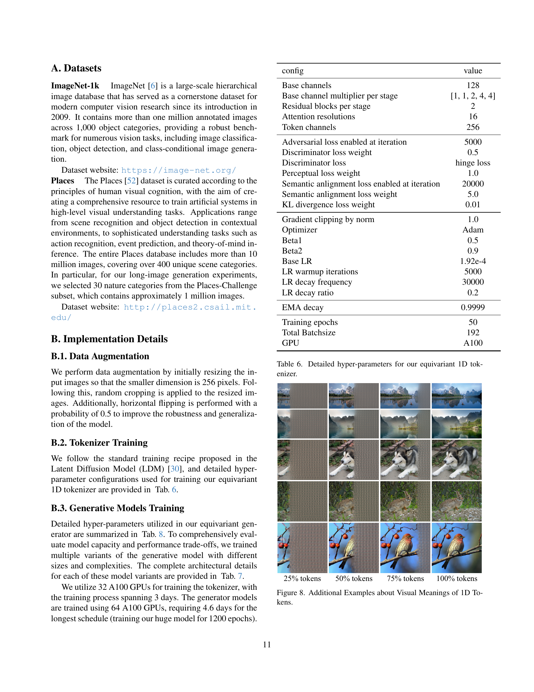
🔼 This figure visualizes the image generation process step by step. Starting from randomly initialized tokens, it progressively replaces these tokens with tokens encoded from the ground truth image. This allows us to see how the decoder faithfully reconstructs the original image, step by step, as the correct token sequences are fed into it. It demonstrates the continuous transition and evolution of the generated image.
read the caption
Figure 9: Visualization of the generation process.

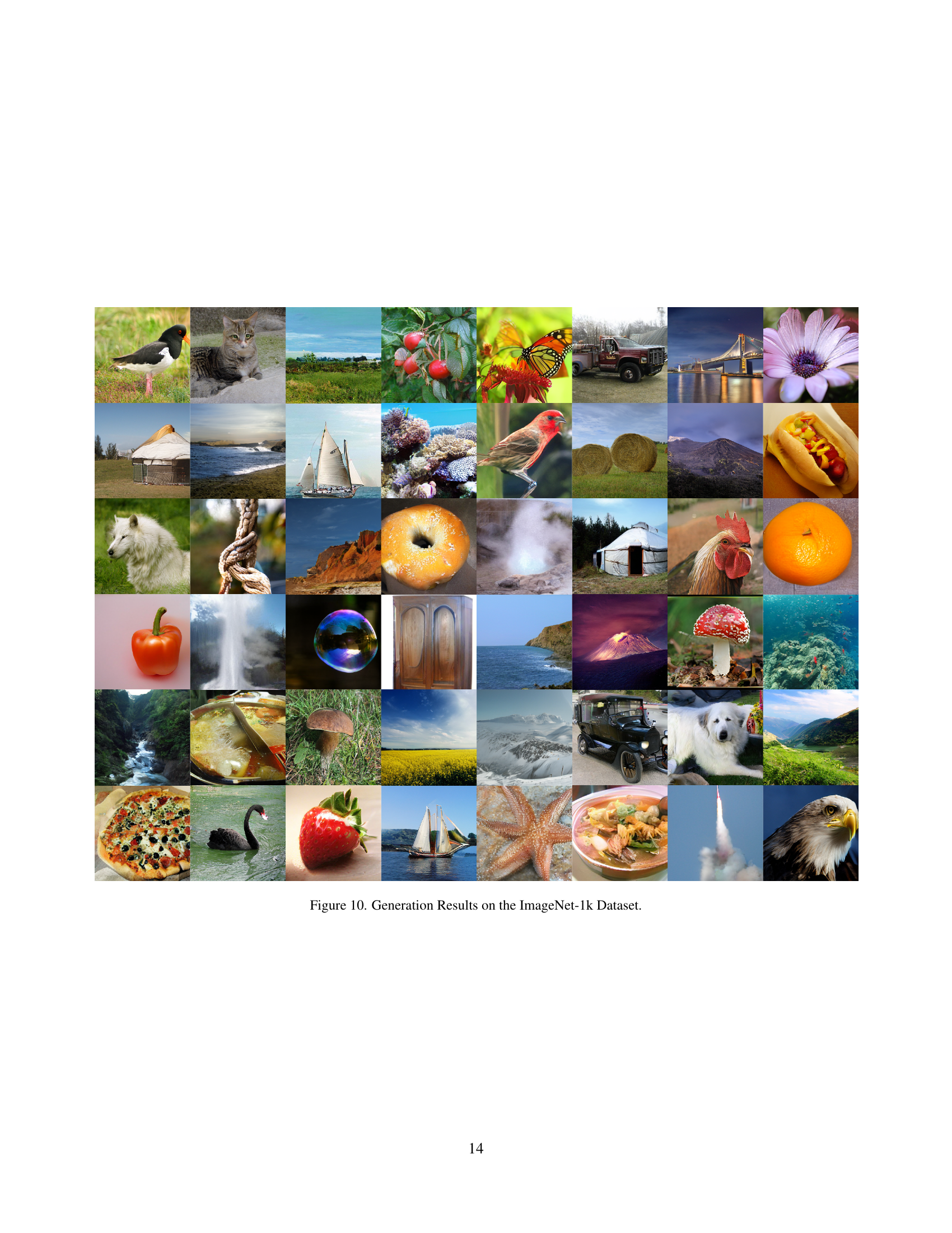
🔼 This figure displays a diverse array of images generated by the model trained on the ImageNet-1k dataset. Each image represents a different object category from the dataset, showcasing the model’s ability to generate various objects with high fidelity and detail. The figure demonstrates the model’s capacity for class-conditional image generation, highlighting the quality and diversity of the generated samples.
read the caption
Figure 10: Generation Results on the ImageNet-1k Dataset.
More on tables
| Method | gFID | IS | #Para. | #Len. | GFLOPs |
| Diffusion | |||||
| DiT [26] | 2.27 | 278.2 | 675M | - | 118.64 |
| MaskGIT | |||||
| TiTok [46] | 1.97 | 281.8 | 287M | 128 | 37.35 |
| MAR [18] | 1.78 | 296.0 | 479M | 64 | 70.13 |
| FractalMAR [17] | 7.30 | 334.9 | 438M | - | 238.58 |
| Autoregressive | |||||
| VQGAN [7] | 15.78 | 74.3 | 1.4B | 256 | 246.67 |
| VAR [40] | 3.30 | 274.4 | 310M | 680 | 105.70 |
| MAR [18] | 4.69 | 244.6 | 479M | 64 | 78.50 |
| Ours-S | 7.21 | 233.70 | 151M | 16 | 5.41 |
| Ours-B | 5.57 | 260.05 | 294M | 16 | 9.78 |
| Ours-L | 4.48 | 259.91 | 644M | 16 | 19.66 |
| Ours-H | 4.17 | 290.66 | 1.2B | 16 | 34.91 |
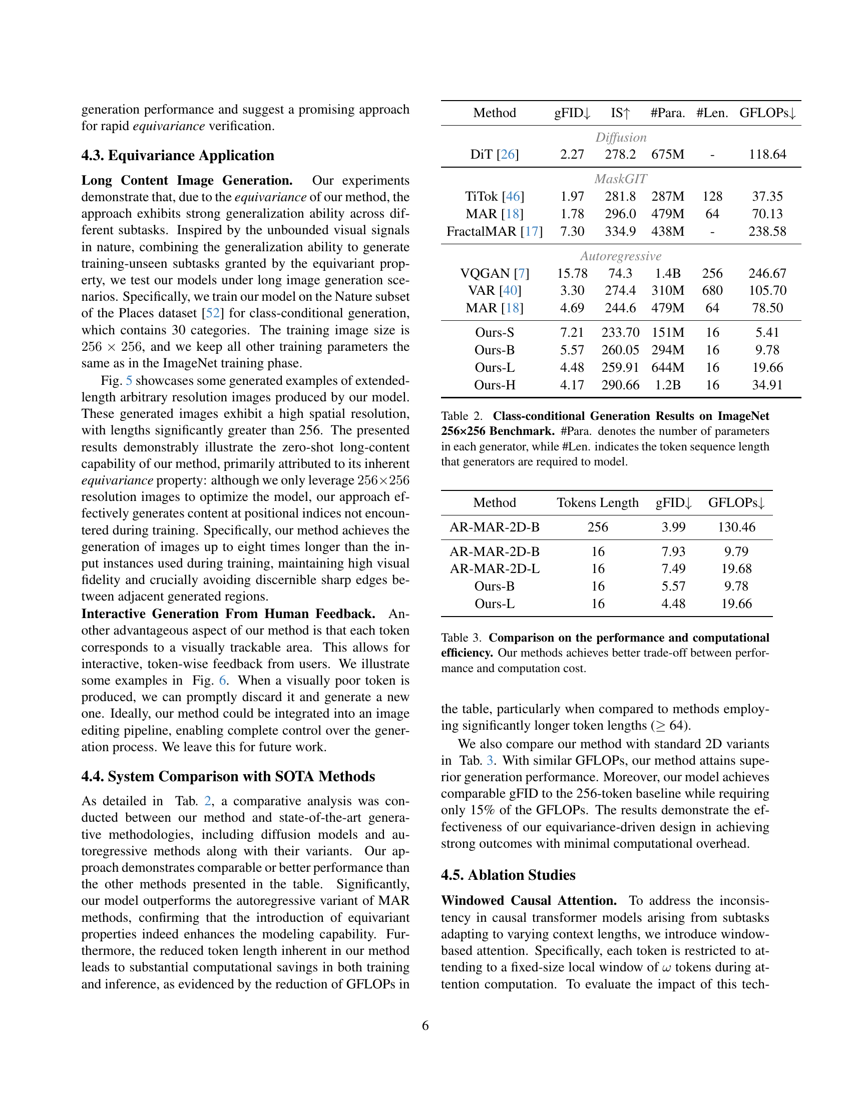
🔼 This table presents the results of class-conditional image generation experiments conducted on the ImageNet dataset at 256x256 resolution. Several different generative models were compared, and the table shows key performance metrics including the Fréchet Inception Distance (gFID), which measures the quality of the generated images, and the Inception Score (IS), which assesses the diversity and quality of the generated images. The table also lists the number of parameters (#Para.) in each model, providing an indication of model complexity, and the token sequence length (#Len.) used by each model during the generation process. Lower gFID and higher IS values generally indicate better performance.
read the caption
Table 2: Class-conditional Generation Results on ImageNet 256×256 Benchmark. #Para. denotes the number of parameters in each generator, while #Len. indicates the token sequence length that generators are required to model.
| Method | Tokens Length | gFID | GFLOPs |
|---|---|---|---|
| AR-MAR-2D-B | 256 | 3.99 | 130.46 |
| AR-MAR-2D-B | 16 | 7.93 | 9.79 |
| AR-MAR-2D-L | 16 | 7.49 | 19.68 |
| Ours-B | 16 | 5.57 | 9.78 |
| Ours-L | 16 | 4.48 | 19.66 |
🔼 This table compares the performance (in terms of gFID) and computational efficiency (GFLOPs) of different models for image generation. It highlights the trade-off between these two aspects. The models compared include the baseline autoregressive models with different token lengths (256 and 16) and the proposed equivariant models with token lengths of 16. The results show that the proposed equivariant models achieve a better trade-off, offering comparable or better performance with significantly reduced computational cost.
read the caption
Table 3: Comparison on the performance and computational efficiency. Our methods achieves better trade-off between performance and computation cost.
| Method | Equ. | L-Ctx. | gFID | Attn FLOPs |
|---|---|---|---|---|
| Full Causal | ✓ | 7.35 | 4.2M | |
| Real Equ. | ✓ | 8.87 | 0.26M | |
| Window Causal | ✓ | ✓ | 7.21 | 1.8M |
🔼 This table presents an ablation study on the impact of windowed causal attention in an equivariant autoregressive image generation model. It compares four different model variations: a baseline model with full causal attention, a strictly equivariant model (Real Equ.) with a limited context window, a model using windowed causal attention, and a model with windowed causal attention and long-range context. The table shows the gFID (lower is better), a measure of image generation quality, and the attention FLOPs (floating-point operations, lower is better), representing computational cost. This allows for an analysis of the trade-off between model performance and computational efficiency when employing different attention mechanisms and degrees of equivariance.
read the caption
Table 4: Ablation Study of Windowed Causal Attention. ”Real Equ.” indicates the strictly equivariant model variant as described in Sec. 3.2; ”Equ.” refers to whether the model possesses equivariant properties; and ”L-Ctx.” denotes whether long-range contexts are utilized.
| Method | rFID | gFID | |
|---|---|---|---|
| 1 | baseline | 1.11 | 7.10 |
| 2 | +Stronger discriminator | 0.62 | 6.29 |
| 3 | + Decoder finetune | 0.58 | 6.25 |
| Ours | +Semantic aligned loss | 0.56 | 5.57 |
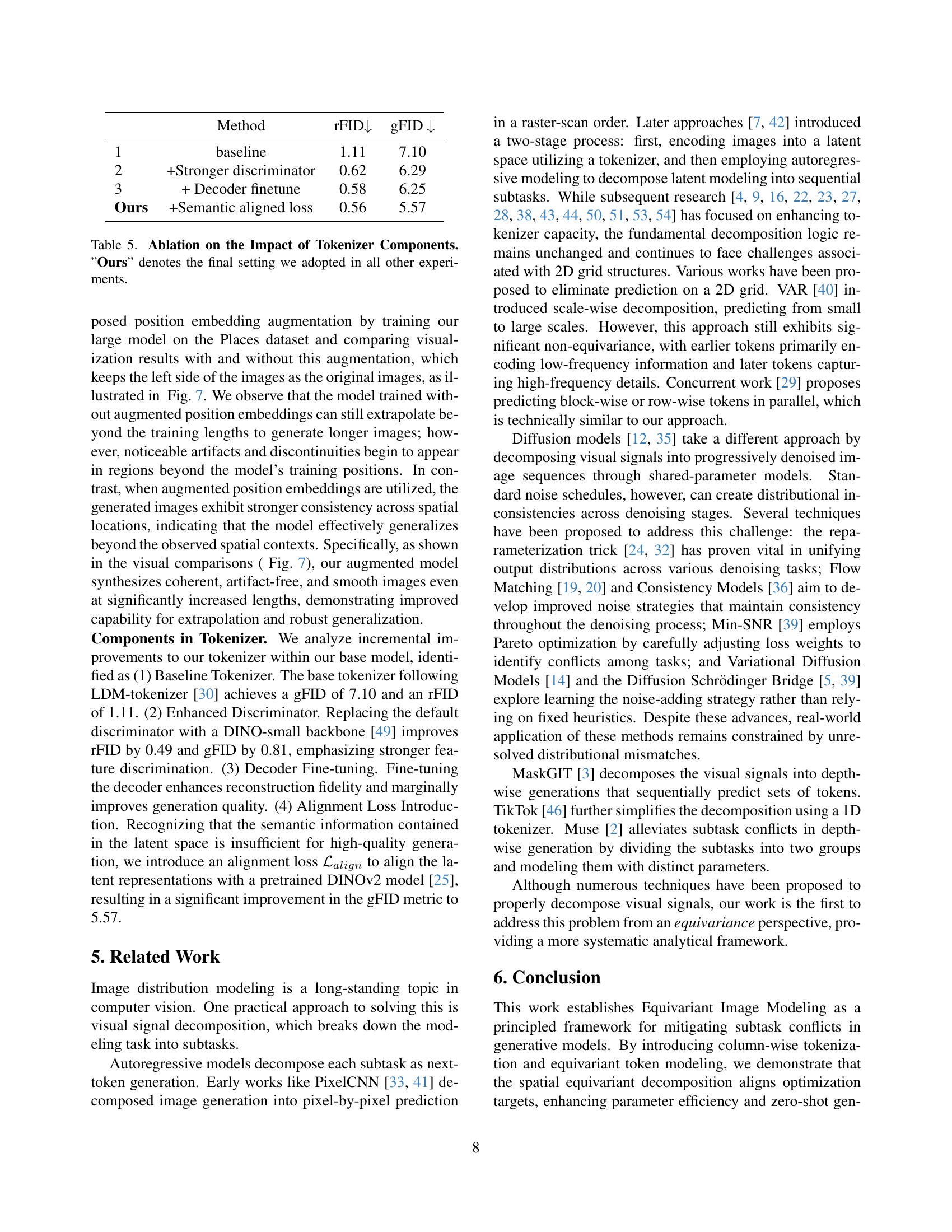
🔼 This table presents the results of ablation experiments performed to evaluate the impact of different components within the tokenizer on the overall model performance. The baseline model is compared against variations that include a stronger discriminator, decoder fine-tuning, and the addition of a semantic alignment loss. The ‘Ours’ row represents the final model configuration that incorporates all of these improvements, and was used in all other experiments in the paper. The table shows the resulting rFID and gFID scores for each variation, demonstrating how the incremental improvements affect the model’s performance in reconstruction fidelity and sample quality.
read the caption
Table 5: Ablation on the Impact of Tokenizer Components. ”Ours” denotes the final setting we adopted in all other experiments.
| config | value |
|---|---|
| Base channels | 128 |
| Base channel multiplier per stage | [1, 1, 2, 4, 4] |
| Residual blocks per stage | 2 |
| Attention resolutions | 16 |
| Token channels | 256 |
| Adversarial loss enabled at iteration | 5000 |
| Discriminator loss weight | 0.5 |
| Discriminator loss | hinge loss |
| Perceptual loss weight | 1.0 |
| Semantic anlignment loss enabled at iteration | 20000 |
| Semantic anlignment loss weight | 5.0 |
| KL divergence loss weight | 0.01 |
| Gradient clipping by norm | 1.0 |
| Optimizer | Adam |
| Beta1 | 0.5 |
| Beta2 | 0.9 |
| Base LR | 1.92e-4 |
| LR warmup iterations | 5000 |
| LR decay frequency | 30000 |
| LR decay ratio | 0.2 |
| EMA decay | 0.9999 |
| Training epochs | 50 |
| Total Batchsize | 192 |
| GPU | A100 |
🔼 This table lists the hyperparameters used during training of the Equivariant 1D tokenizer, a key component in the proposed image generation framework. It details settings for various aspects of the training process, including network architecture (base channels, residual blocks, attention resolutions), loss functions (adversarial, discriminator, perceptual, semantic alignment, KL divergence), optimization parameters (optimizer, learning rate, decay, warmup, and EMA), and training schedule (epochs, batch size). These values were carefully chosen to optimize the performance of the tokenizer in preparing the image data for the subsequent generative model.
read the caption
Table 6: Detailed hyper-parameters for our equivariant 1D tokenizer.
| Model | #Para. | Layers | Hidden dim | Attn heads | Diff. hidden dim | Diff.layers |
|---|---|---|---|---|---|---|
| Small | 151M | 16 | 512 | 8 | 960 | 12 |
| Base | 294M | 24 | 768 | 12 | 1024 | 12 |
| Large | 644M | 32 | 1024 | 16 | 1280 | 12 |
| Huge | 1.2B | 40 | 1280 | 16 | 1536 | 12 |
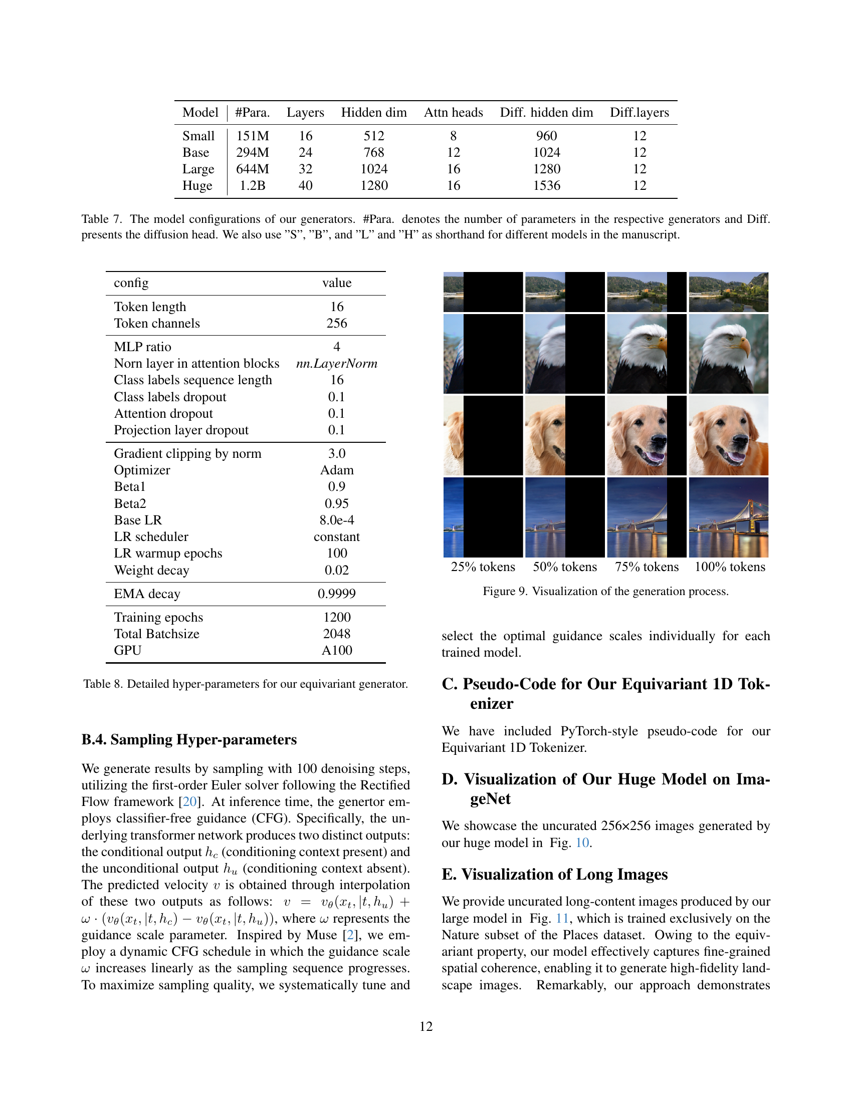
🔼 This table details the architecture specifications for four different image generation models (Small, Base, Large, and Huge). For each model, it lists the number of parameters (#Para.), the number of layers, the hidden dimension size, the number of attention heads, the diffusion hidden dimension size, and the number of diffusion layers. The ‘Diff.’ column refers to the diffusion head, a component of the model used for image generation. The table also notes that ‘S’, ‘B’, ‘L’, and ‘H’ are used in the paper as shorthand for Small, Base, Large, and Huge respectively.
read the caption
Table 7: The model configurations of our generators. #Para. denotes the number of parameters in the respective generators and Diff. presents the diffusion head. We also use ”S”, ”B”, and ”L” and ”H” as shorthand for different models in the manuscript.
| config | value |
|---|---|
| Token length | 16 |
| Token channels | 256 |
| MLP ratio | 4 |
| Norn layer in attention blocks | nn.LayerNorm |
| Class labels sequence length | 16 |
| Class labels dropout | 0.1 |
| Attention dropout | 0.1 |
| Projection layer dropout | 0.1 |
| Gradient clipping by norm | 3.0 |
| Optimizer | Adam |
| Beta1 | 0.9 |
| Beta2 | 0.95 |
| Base LR | 8.0e-4 |
| LR scheduler | constant |
| LR warmup epochs | 100 |
| Weight decay | 0.02 |
| EMA decay | 0.9999 |
| Training epochs | 1200 |
| Total Batchsize | 2048 |
| GPU | A100 |
🔼 This table details the hyperparameters used for training the equivariant generator model. It lists the settings for various aspects of the training process, including tokenization parameters (token length and channels), network architecture choices (MLP ratio, normalization layers, dropout rates), optimization settings (optimizer, learning rate schedule, weight decay), and other regularization techniques.
read the caption
Table 8: Detailed hyper-parameters for our equivariant generator.
Full paper#