TL;DR#
Computer vision models often exhibit biases, leading to unfair or inaccurate outcomes. Current methods for detecting these biases primarily focus on overall performance and data distribution, but they often overlook the internal workings of the model. This can result in an incomplete understanding of how biases are formed and propagated.
The paper introduces the Attention-IoU metric, which uses attention maps to reveal biases within a model’s internal representations. By comparing these maps with ground-truth feature masks or attention maps of other attributes, Attention-IoU quantifies how a model relies on specific image regions. This allows for the identification of spurious correlations and potential confounding variables, leading to more effective debiasing techniques.The metric is validated through the use of the synthetic Waterbirds dataset as well as the popular CelebA dataset.
Key Takeaways#
Why does it matter?#
This paper is important for researchers because it introduces a novel metric for identifying and understanding biases in computer vision models. This work opens new avenues for developing more robust and fair AI systems by providing a more nuanced way to evaluate model behavior and uncover potential confounding variables.
Visual Insights#

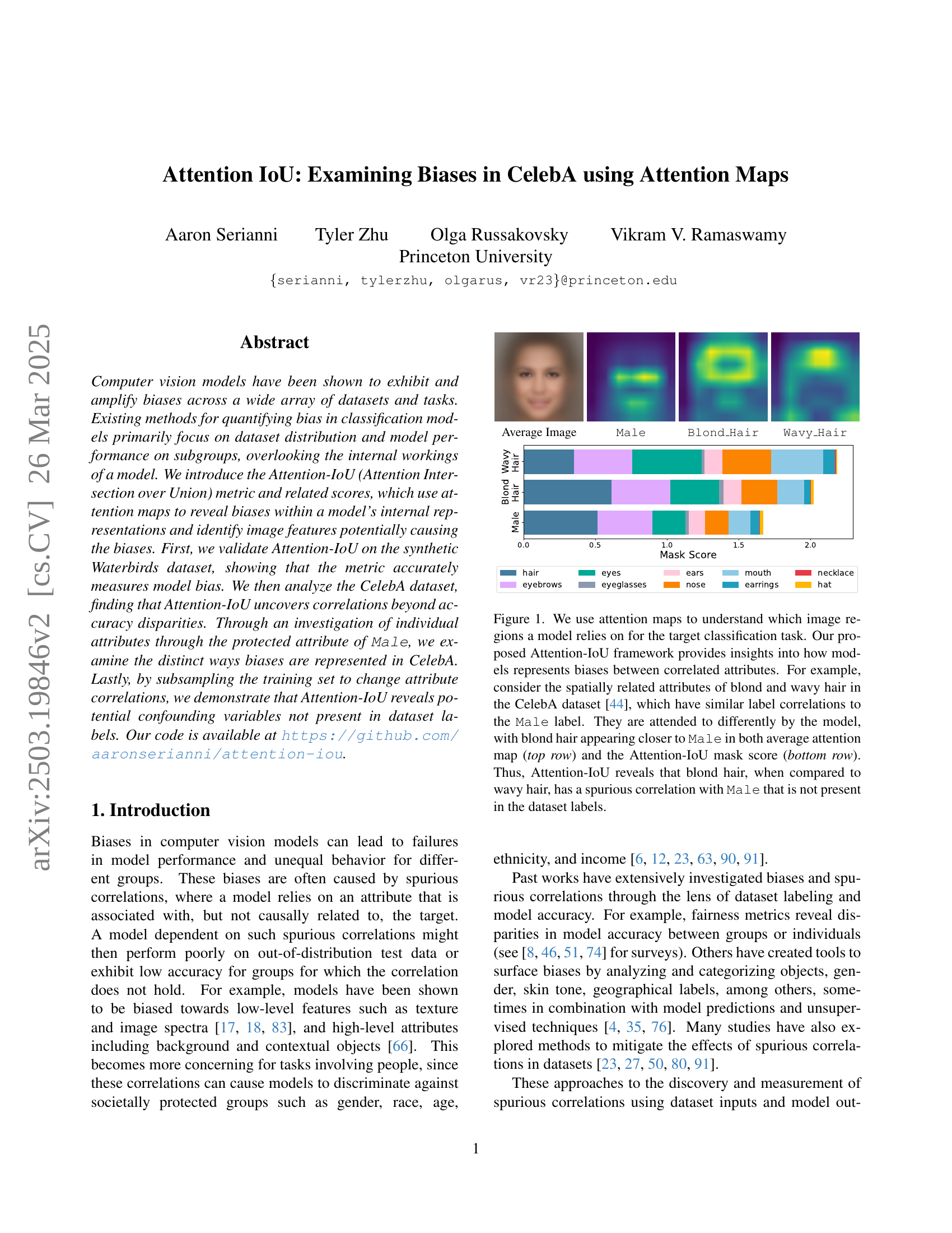
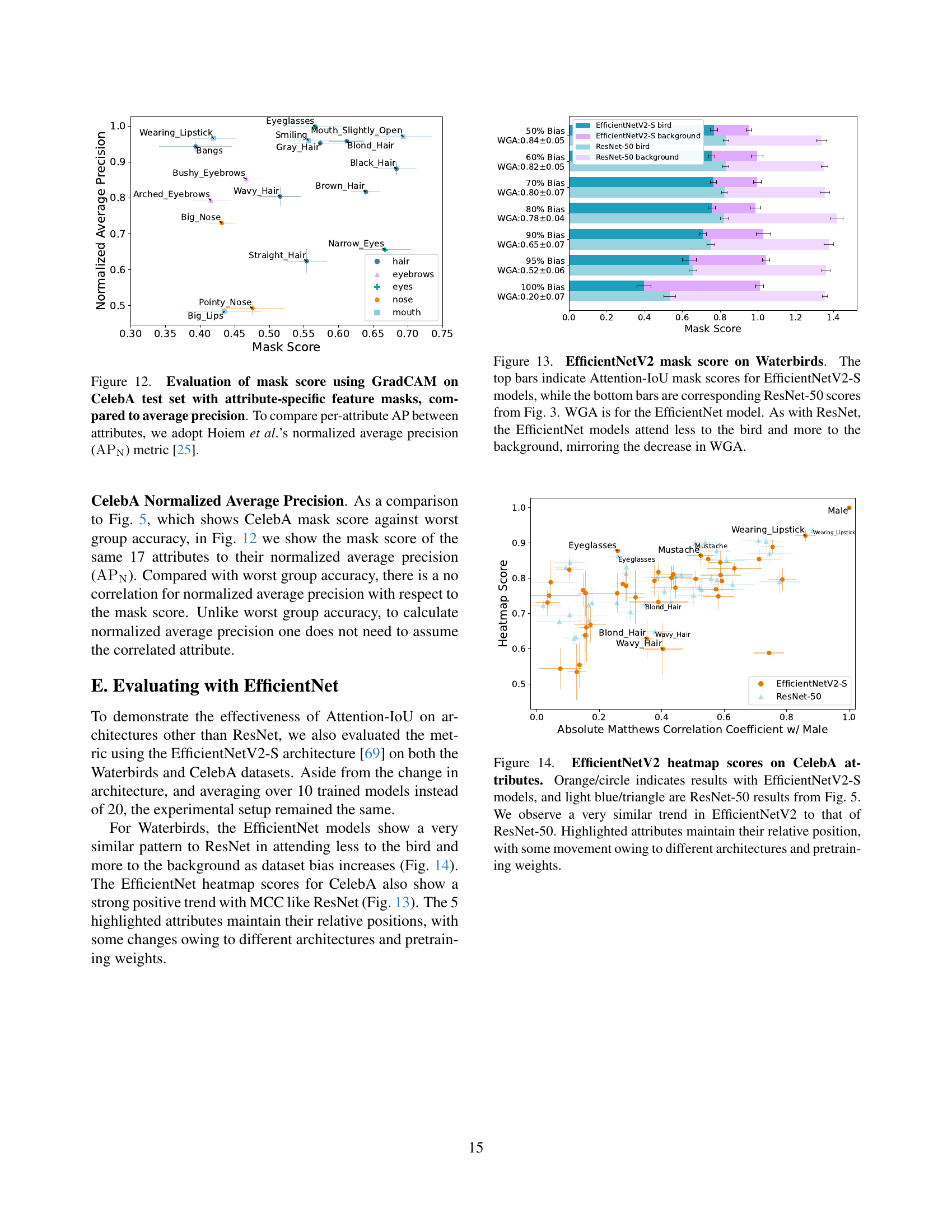
🔼 This figure visualizes the average face image from the CelebA dataset, along with attention maps highlighting regions focused on by a model when classifying different attributes. These attributes include ‘Male’, ‘Blond Hair’, and ‘Wavy Hair.’ The attention maps reveal the model’s reliance on certain facial features (like hair) for specific attribute classifications and potentially expose correlations between attributes, which may reveal underlying biases. Specifically, the attention for ‘Blond Hair’ is compared to that of ‘Wavy Hair’ to illustrate spurious correlation with ‘Male’, something not explicitly present in the dataset labels alone.
read the caption
Average Image
In-depth insights#
Attention Bias#
Attention bias, a cognitive phenomenon where individuals selectively focus on certain stimuli while ignoring others, plays a crucial role in how AI models learn and perpetuate biases. In computer vision, models may exhibit attention bias by disproportionately attending to specific image features associated with protected attributes like gender or race. This selective attention can lead to spurious correlations, where models rely on features that are not causally related to the target task, resulting in discriminatory outcomes. For example, if a model trained to identify ‘blond hair’ focuses on gendered aspects of faces rather than hair features, it perpetuates gender bias. Methods like Attention-IoU help to reveal these biases by quantifying how much a model’s attention overlaps with confounding attributes, offering insights for developing more equitable and robust AI systems by identifying the image regions driving biased predictions.
Attention-IoU#
The name ‘Attention-IoU’ is catchy, hinting at the core concept of using attention mechanisms and Intersection over Union (IoU), a metric for measuring the overlap between predicted and ground truth regions. The technique could focus on analyzing attention maps generated by models to identify areas of the input image that the model focuses on when making predictions. By comparing these attention maps, likely across different groups or attributes, the IoU metric would then quantify the extent to which the model’s attention overlaps, revealing potential biases. A high IoU between attention maps for different attributes would suggest that the model relies on similar image regions for both, indicating a potential confounding relationship or a bias. This approach offers a way to open the ‘black box’ of deep learning models and identify finer-grained biases beyond simple performance disparities.
Mask vs. Heatmap#
In the realm of explainable AI, mask and heatmap techniques serve distinct roles in elucidating model behavior. Masks, often binary, highlight regions deemed most relevant by the model, providing a clear focus on specific image areas. They are useful for isolating key features and quantifying their impact. Heatmaps, conversely, offer a more nuanced, continuous representation of feature importance. By assigning varying intensities to different regions, heatmaps reveal the subtle gradations of influence, showcasing the relative contributions of various image parts. Masks are better for clearly isolating the key feature and heatmap shows nuanced relation. While masks provide a definitive ‘yes’ or ’no’ assessment of relevance, heatmaps offer a richer, more contextual understanding of the model’s decision-making process. The choice depends on the goal, either clearly isolating a feature with a mask or knowing a more granular relation with a heatmap.
CelebA Analysis#
Analyzing CelebA reveals insights beyond accuracy disparities. Attention-IoU identifies how the ‘Male’ attribute influences others. Some attributes are unevenly affected, and biases exceed dataset label correlations. This reveals nuanced biases in how models perceive attributes like gender and its relation to other facial features. The study uses CelebAMask-HQ for detailed facial segmentation. Unlike the synthetic Waterbirds dataset, CelebA’s biases aren’t directly tied to a single attribute. Heatmap analysis highlights regions models focus on, linking attention to spurious correlations. It compares feature mask scores and worst-group accuracy, showing that attribute bias depends on image features and label distribution with other attributes. The research finds a strong positive trend between heatmap score and predicted label correlation (MCC). Outliers like Mustache and Eyeglasses indicate unique biases.
Future Metrics#
Future metrics should go beyond traditional accuracy measures. Interpretability-focused metrics are crucial, quantifying how well a model’s internal reasoning aligns with human understanding. Metrics capturing fairness across intersectional groups are vital to reveal nuanced biases. Furthermore, metrics should assess model robustness to distribution shifts and adversarial attacks, ensuring reliability in real-world scenarios. Developing metrics that effectively incorporate causal reasoning would also significantly advance bias detection. Finally, future work may focus on fine-grained metrics to evaluate the contribution of individual features.
More visual insights#
More on figures

🔼 This figure displays average attention maps for the ‘Male’ attribute in the CelebA dataset, highlighting the image regions the model focuses on when predicting this attribute. Each sub-image represents the average attention map generated by the model across all instances of the images in the dataset. Regions with brighter intensity indicate higher attention weights, revealing the model’s reliance on specific facial features to determine gender. The figure likely shows the visual evidence supporting a claim that the model’s prediction is biased toward specific visual cues, rather than the underlying attribute itself. For example, if brighter areas strongly correlate with non-facial, correlated attributes (hair style, makeup, etc.), it would suggest that the model is relying on spurious correlations rather than true gender characteristics.
read the caption
Male

🔼 This figure visualizes average heatmaps for the ‘Blond Hair’ attribute in the CelebA dataset using the Attention-IoU method. Different heatmaps are shown for various scenarios depending on the values of ‘Male’ and ‘Mustache’ attributes. Comparing these heatmaps allows for analysis of how the model attends to different facial regions when predicting the ‘Blond Hair’ attribute, revealing potential biases and spurious correlations within the model’s internal representations.
read the caption
Blond_Hair
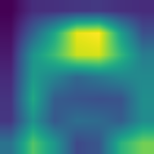
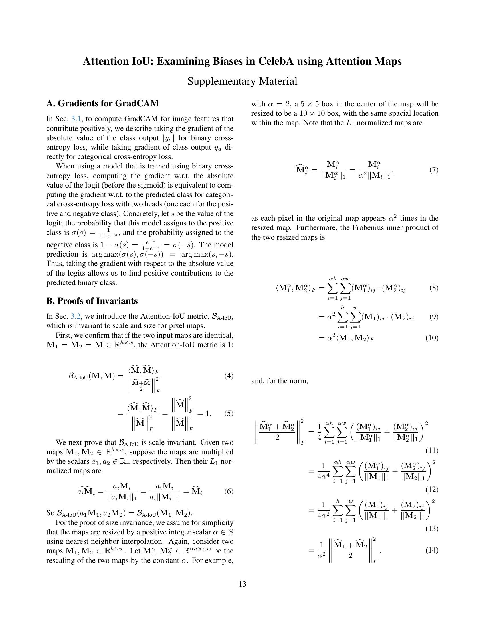
🔼 This figure shows the average attention map (heatmap) for the attribute ‘Wavy Hair’ as generated by GradCAM using a model trained on the CelebA dataset. The heatmap visually represents which parts of the input image the model focuses on most strongly when determining whether an image depicts wavy hair. Brighter regions in the heatmap indicate higher attention weights assigned by the model to those specific image areas. This visualization helps to understand the model’s internal decision-making process regarding this attribute and can potentially reveal any biases or spurious correlations the model may be relying on.
read the caption
Wavy_Hair

🔼 This figure demonstrates how Attention-IoU can reveal biases in a model’s internal representations by analyzing attention maps. The top row shows average attention maps for different attributes (blond hair, wavy hair, and male) in the CelebA dataset. The bottom row shows Attention-IoU mask scores, quantifying the correlation between these attributes. The example highlights that although blond and wavy hair have similar correlations with the ‘male’ label in the dataset, the model attends to blond hair more strongly when predicting ‘male’, revealing a spurious correlation not reflected in the dataset labels themselves. This spurious correlation is detected through the difference in attention patterns, illustrating how Attention-IoU reveals biases beyond simple accuracy disparities.
read the caption
Figure 1: We use attention maps to understand which image regions a model relies on for the target classification task. Our proposed Attention-IoU framework provides insights into how models represents biases between correlated attributes. For example, consider the spatially related attributes of blond and wavy hair in the CelebA dataset [44], which have similar label correlations to the Male label. They are attended to differently by the model, with blond hair appearing closer to Male in both average attention map (top row) and the Attention-IoU mask score (bottom row). Thus, Attention-IoU reveals that blond hair, when compared to wavy hair, has a spurious correlation with Male that is not present in the dataset labels.

🔼 This figure illustrates the concept of background bias in image classification models. It uses the Waterbirds dataset, where images of waterbirds are often associated with water backgrounds and landbirds with land backgrounds. The figure displays three examples of how a model might erroneously rely on the background rather than the bird itself to make its classification. Panel (a) shows a model attending to the entire background, Panel (b) focusing on a ship in the background rather than the bird, and panel (c) only on part of the bird’s wing (indicating an incomplete or incorrect recognition of the actual object of classification). These examples highlight different ways spurious correlations can lead to bias, where the model relies on information associated with, but not inherently predictive of, the correct class.
read the caption
Background Bias

🔼 The figure illustrates a type of model bias where the model attends to an object other than the target object for classification. In the example, the model incorrectly focuses on a ship in the background instead of correctly identifying the landbird, resulting in an erroneous classification.
read the caption
Object Bias

🔼 The figure illustrates the concept of ‘Depiction Bias’ in computer vision models, where the model’s performance is affected not by the object itself but by how it is depicted in the image. It shows three examples of attention maps generated by a model trying to classify a landbird on a water background. In the first example, the model mistakenly focuses on the entire background (the water) when classifying the bird. In the second, the model focuses on a ship (a spurious feature associated with the background) rather than the bird itself. In the third, the model only attends to a small part of the bird (its wing), potentially leading to misclassification due to the incomplete depiction of the bird.
read the caption
Depiction Bias

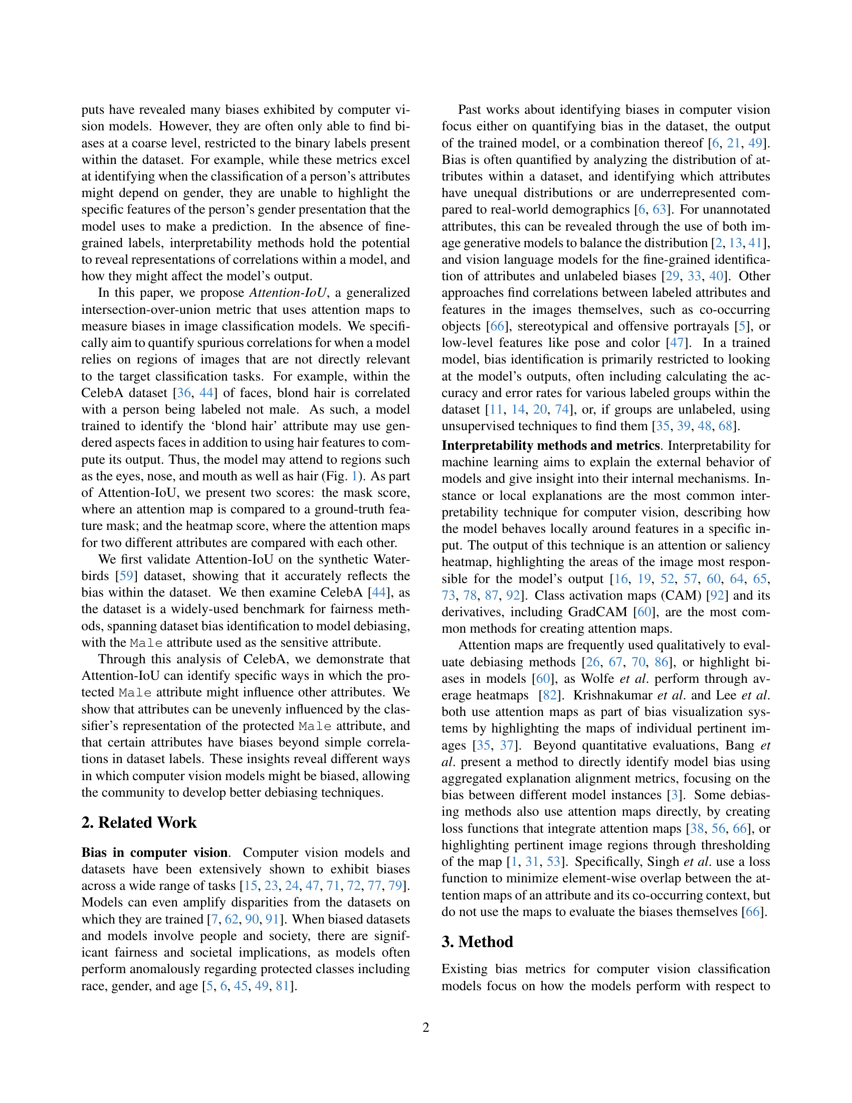
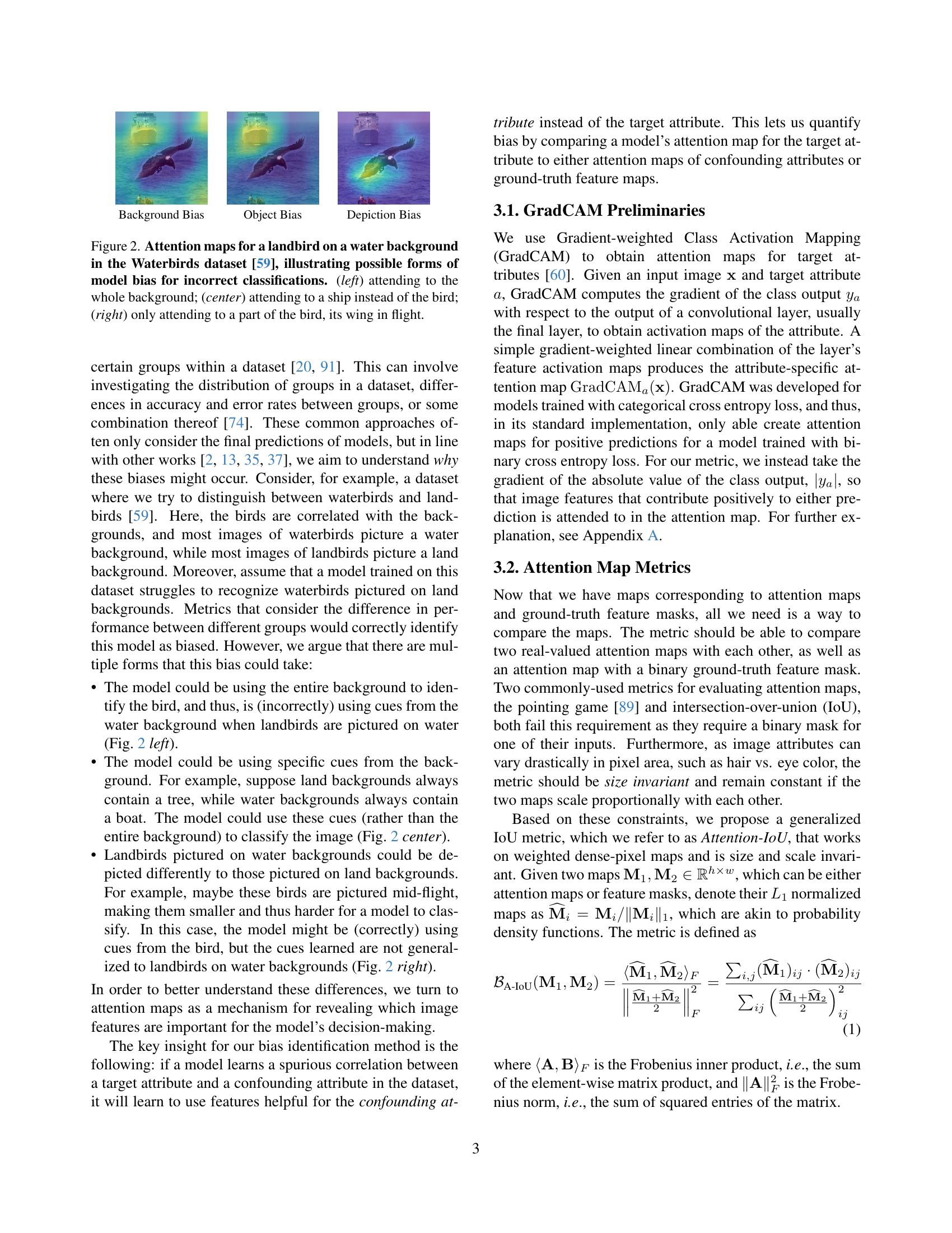
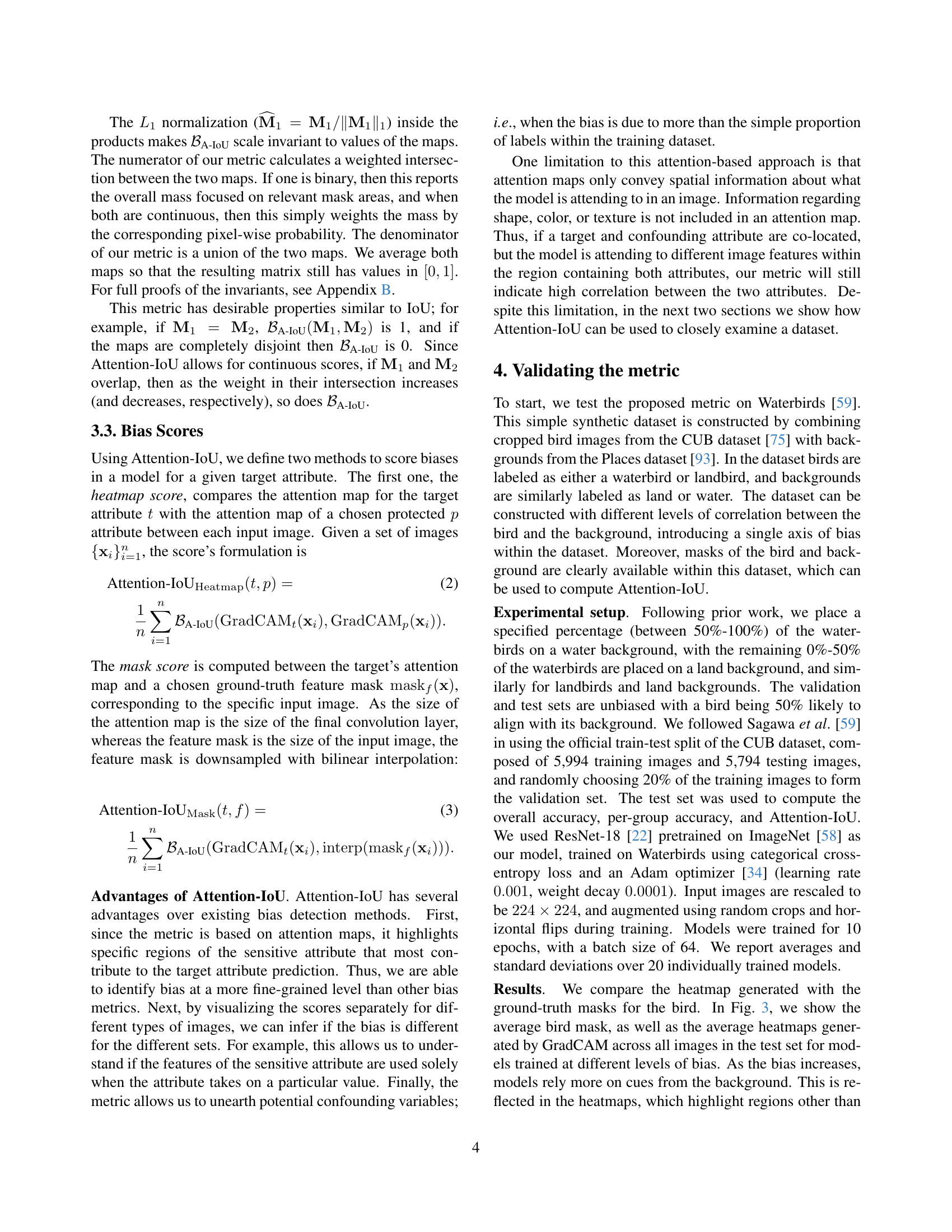
🔼 Figure 2 illustrates different ways a model can exhibit bias when classifying images from the Waterbirds dataset. The example shows a landbird incorrectly classified, possibly due to the model focusing on irrelevant features. The image on the left shows the model attending to the entire background, suggesting it might be relying on spurious correlations between the bird type and background rather than the bird itself. The center image shows the model incorrectly focusing on a ship in the background, again indicating spurious correlation bias. The image on the right shows the model only attending to a small portion of the bird (its wing), suggesting the model might be learning from incomplete or low-level features rather than the whole object.
read the caption
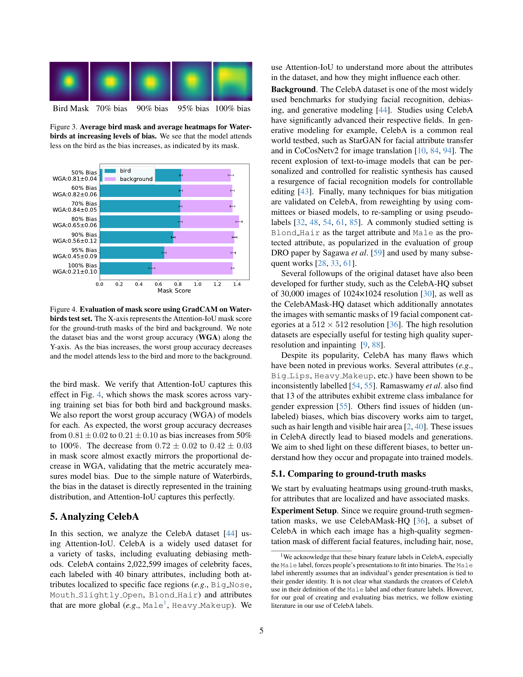
Figure 2: Attention maps for a landbird on a water background in the Waterbirds dataset [59], illustrating possible forms of model bias for incorrect classifications. (left) attending to the whole background; (center) attending to a ship instead of the bird; (right) only attending to a part of the bird, its wing in flight.

🔼 This figure visualizes the impact of increasing bias in the Waterbirds dataset on a model’s attention. The leftmost panel shows the ground truth mask of a bird. The subsequent panels display average GradCAM attention maps for models trained on datasets with progressively higher levels of spurious correlation between birds and their backgrounds (70%, 90%, 95%, 100% bias). As the bias increases (more spurious correlations), the heatmaps clearly show a shift in the model’s focus, from attending primarily to the bird itself to increasingly attending to the background, indicating that the model relies more heavily on spurious correlations for classification as bias increases. This is reflected in the decreasing focus on the bird region as indicated by its mask.
read the caption
Figure 3: Average bird mask and average heatmaps for Waterbirds at increasing levels of bias. We see that the model attends less on the bird as the bias increases, as indicated by its mask.

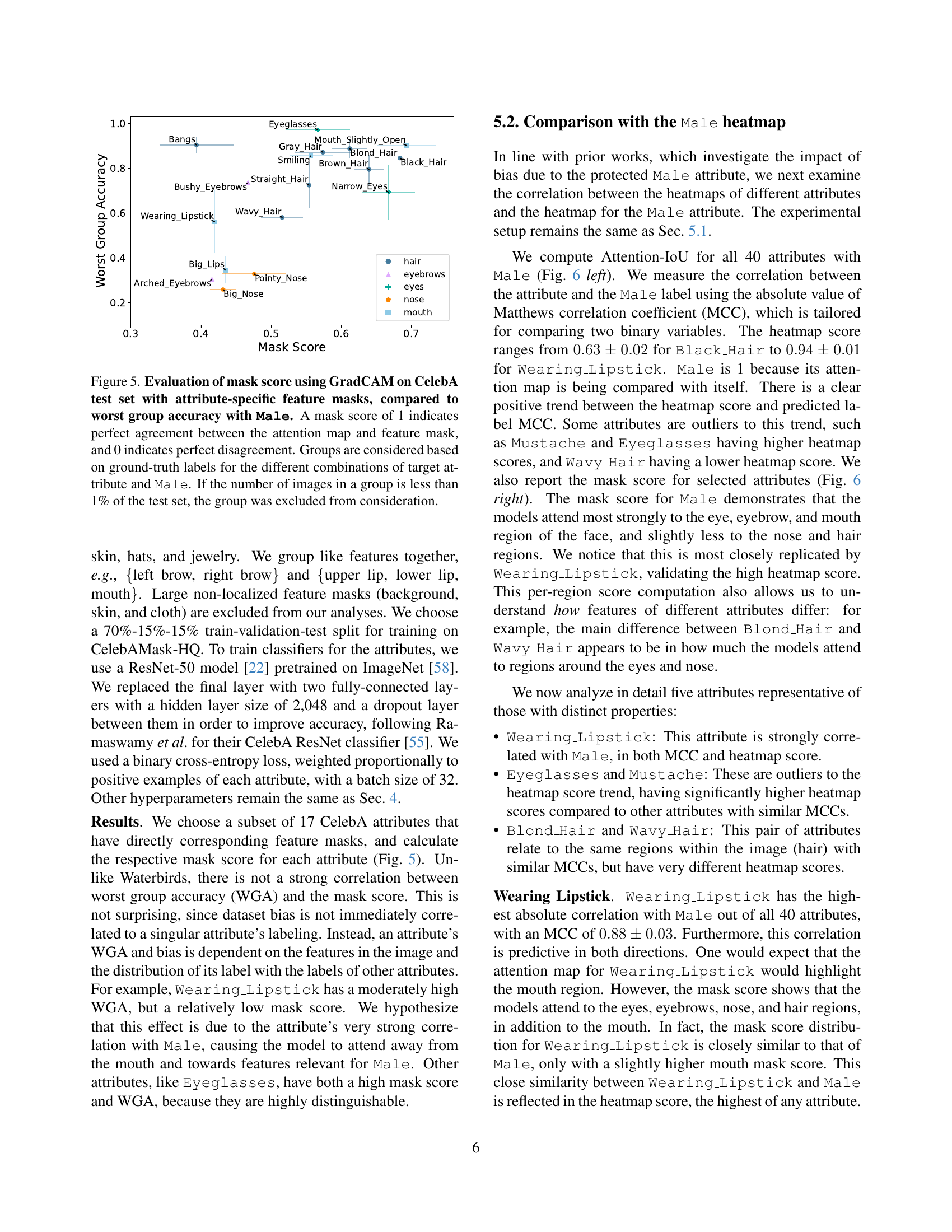
🔼 This figure displays the relationship between dataset bias, model performance, and attention mechanisms. The x-axis shows the Attention-IoU mask score, which quantifies how well the model’s attention aligns with the ground truth bird and background masks. A higher score indicates better alignment. The y-axis shows both the dataset bias (percentage of waterbirds on water backgrounds) and the worst-group accuracy (WGA). The graph demonstrates that as dataset bias increases (more spurious correlations), the worst-group accuracy decreases, and the model’s attention shifts from the bird (the true target) to the background (the spurious correlation). This visually confirms that Attention-IoU effectively measures model bias by reflecting the model’s reliance on spurious correlations.
read the caption
Figure 4: Evaluation of mask score using GradCAM on Waterbirds test set. The X-axis represents the Attention-IoU mask score for the ground-truth masks of the bird and background. We note the dataset bias and the worst group accuracy (WGA) along the Y-axis. As the bias increases, the worst group accuracy decreases and the model attends less to the bird and more to the background.

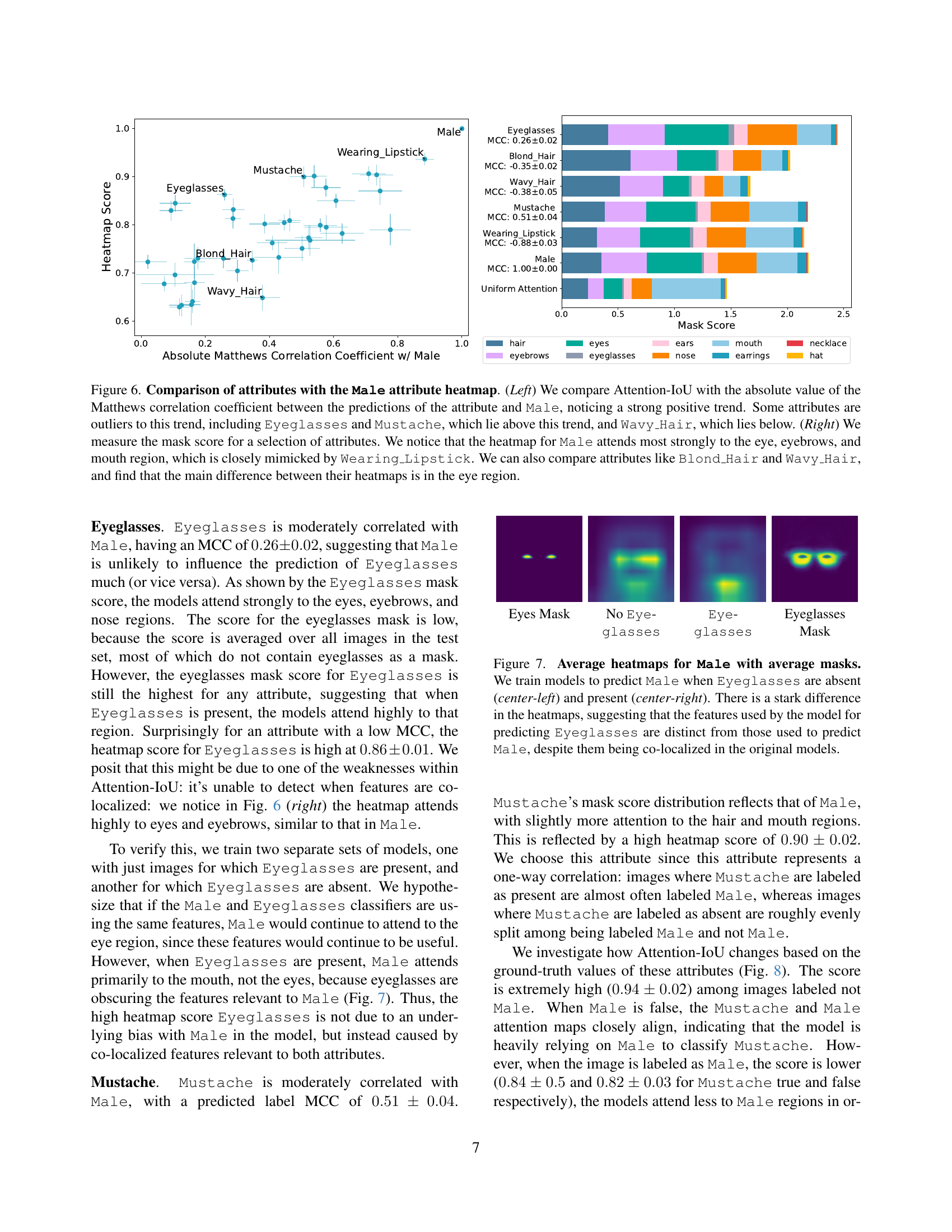
🔼 This figure displays the mask score for different attributes in the CelebA dataset, calculated using GradCAM. The mask score measures the agreement between a model’s attention map and the ground truth feature mask for each attribute. The x-axis shows the mask score, ranging from 0 (perfect disagreement) to 1 (perfect agreement). The y-axis lists the attributes, grouped by their general facial feature category (hair, eyebrows, eyes, etc.). Each dot represents a group of images with a specific combination of the target attribute and the protected attribute of ‘Male’. The size of the dot corresponds to the number of images in that group; groups with fewer than 1% of the total test set images are excluded. The figure also shows the worst-group accuracy (WGA) for each attribute group; thus, demonstrating the relationship between a model’s attention focus and its classification performance on different subgroups, thereby providing insight into potential biases in the model.
read the caption
Figure 5: Evaluation of mask score using GradCAM on CelebA test set with attribute-specific feature masks, compared to worst group accuracy with Male. A mask score of 1 indicates perfect agreement between the attention map and feature mask, and 0 indicates perfect disagreement. Groups are considered based on ground-truth labels for the different combinations of target attribute and Male. If the number of images in a group is less than 1% of the test set, the group was excluded from consideration.

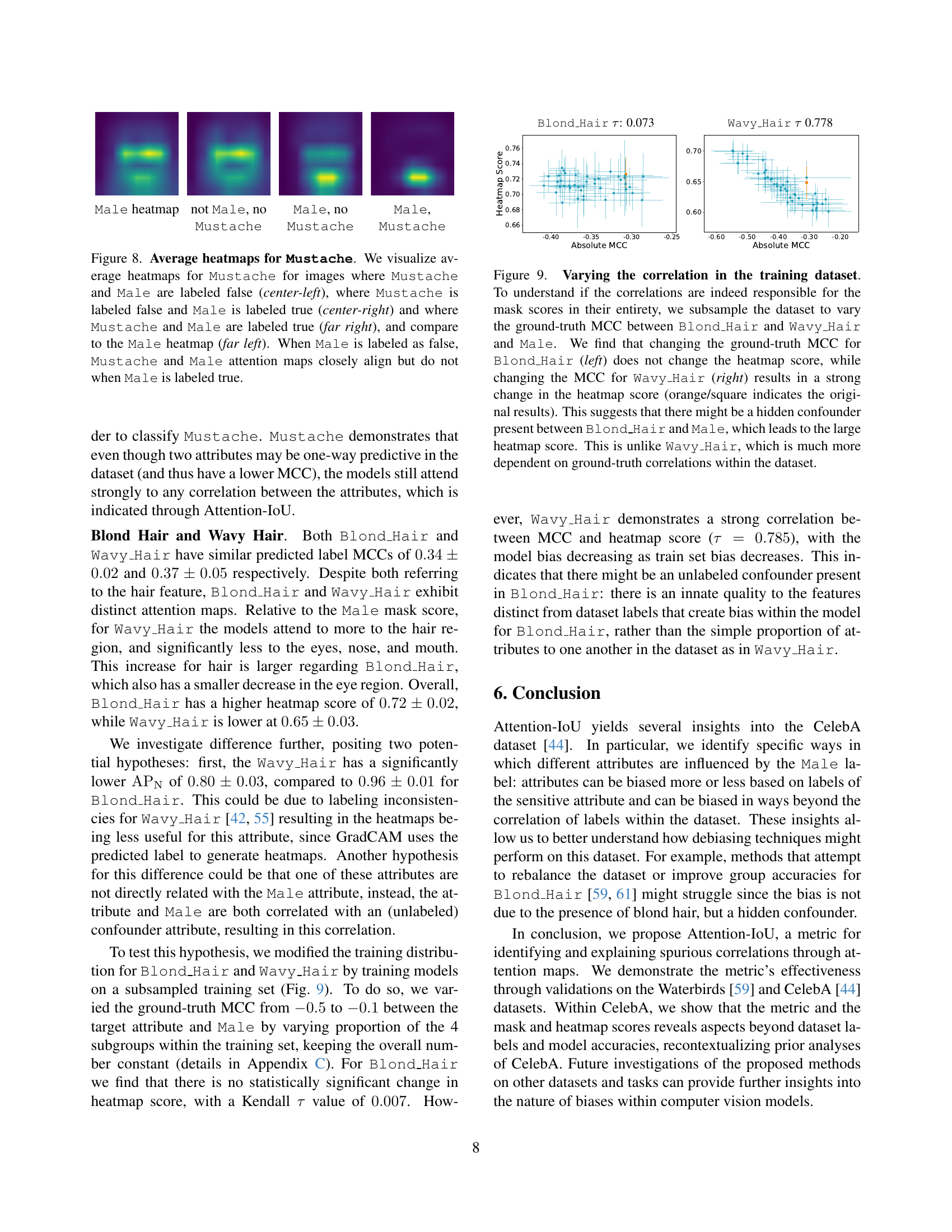
🔼 Figure 6 analyzes the relationship between different facial attributes and the ‘Male’ attribute in the CelebA dataset using the Attention-IoU metric. The left panel shows a strong positive correlation between the Attention-IoU heatmap score (measuring the overlap of attention maps for an attribute and the ‘Male’ attribute) and the absolute value of the Matthews Correlation Coefficient (MCC) between the attribute’s prediction and the ‘Male’ label. However, some attributes like ‘Eyeglasses’ and ‘Mustache’ show higher Attention-IoU scores than expected based on their MCC, while ‘Wavy Hair’ shows a lower score. The right panel displays the mask scores (comparing attention maps to ground truth masks) for several attributes, revealing that the ‘Male’ attribute’s attention map focuses mainly on the eye, eyebrow, and mouth regions, a pattern closely mirrored by ‘Wearing Lipstick’. A comparison of ‘Blond Hair’ and ‘Wavy Hair’ highlights that the key difference in their attention maps lies in the eye region.
read the caption
Figure 6: Comparison of attributes with the Male attribute heatmap. (Left) We compare Attention-IoU with the absolute value of the Matthews correlation coefficient between the predictions of the attribute and Male, noticing a strong positive trend. Some attributes are outliers to this trend, including Eyeglasses and Mustache, which lie above this trend, and Wavy_Hair, which lies below. (Right) We measure the mask score for a selection of attributes. We notice that the heatmap for Male attends most strongly to the eye, eyebrows, and mouth region, which is closely mimicked by Wearing_Lipstick. We can also compare attributes like Blond_Hair and Wavy_Hair, and find that the main difference between their heatmaps is in the eye region.

🔼 This figure visualizes average attention maps for predicting the attribute ‘Male’ under different conditions regarding the presence of ‘Eyeglasses’. By comparing heatmaps from models trained separately on datasets with and without eyeglasses, the figure demonstrates that the model utilizes distinct image features to recognize ‘Male’ when eyeglasses are present versus absent. This highlights that even spatially overlapping attributes can rely on different features leading to potential model biases or spurious correlations.
read the caption
Figure 7: Average heatmaps for Male with average masks. We train models to predict Male when Eyeglasses are absent (center-left) and present (center-right). There is a stark difference in the heatmaps, suggesting that the features used by the model for predicting Eyeglasses are distinct from those used to predict Male, despite them being co-localized in the original models.
🔼 This figure visualizes average attention maps generated by a model for the attribute ‘Mustache’, broken down into four scenarios based on the ground truth labels for ‘Mustache’ and ‘Male’: 1. Male: False, Mustache: False (center-left): Shows the average attention map when neither ‘Male’ nor ‘Mustache’ is present. 2. Male: True, Mustache: False (center): Shows the average attention map when ‘Male’ is present but ‘Mustache’ is not. 3. Male: False, Mustache: True (center-right): Shows the average attention map when ‘Mustache’ is present but ‘Male’ is not. 4. Male: True, Mustache: True (far right): Shows the average attention map when both ‘Male’ and ‘Mustache’ are present. The figure compares these attention maps to the average attention map for ‘Male’ (far left). The key observation is that the attention maps for ‘Mustache’ strongly resemble the ‘Male’ attention map when the ‘Male’ label is false, indicating a potential spurious correlation between the two attributes. However, this correlation disappears when the ‘Male’ label is true, implying that the model uses different features for detecting ‘Mustache’ depending on the gender of the subject.
read the caption
Figure 8: Average heatmaps for Mustache. We visualize average heatmaps for Mustache for images where Mustache and Male are labeled false (center-left), where Mustache is labeled false and Male is labeled true (center-right) and where Mustache and Male are labeled true (far right), and compare to the Male heatmap (far left). When Male is labeled as false, Mustache and Male attention maps closely align but do not when Male is labeled true.
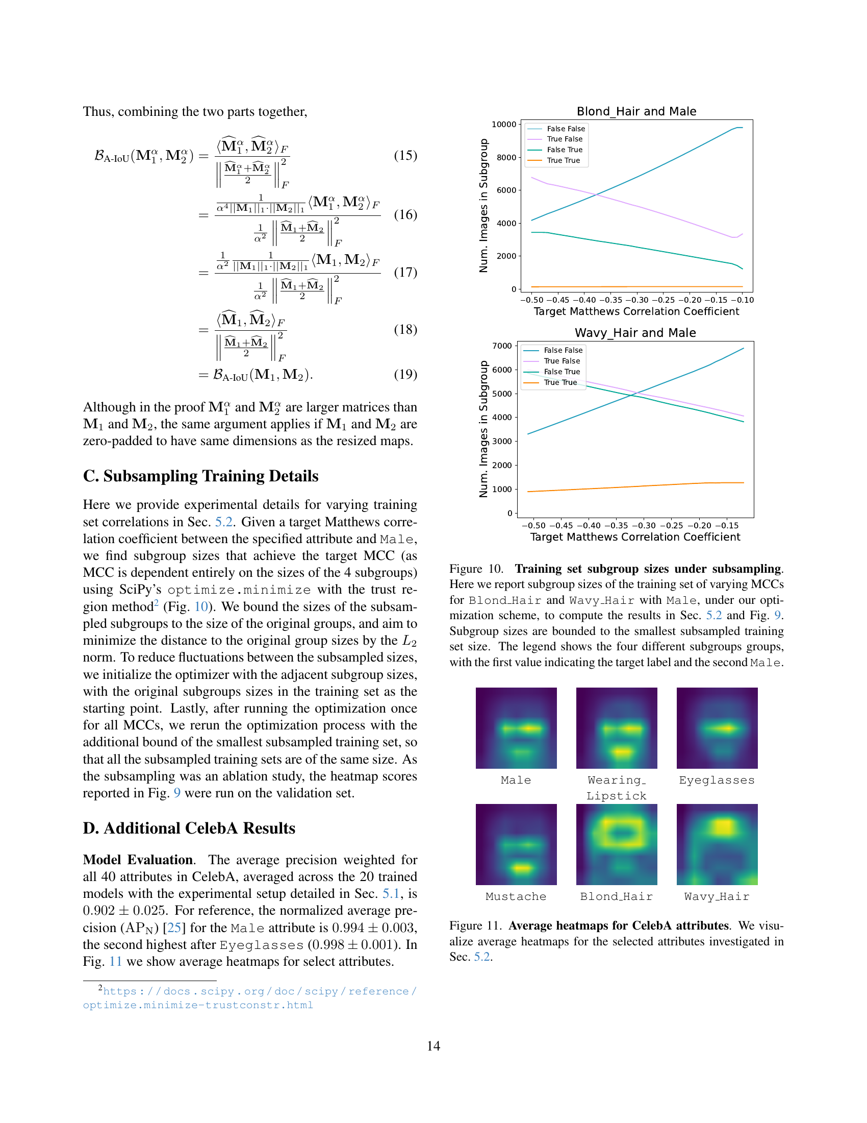
🔼 This figure visualizes the effect of subsampling the training dataset to manipulate the correlation between the Blond_Hair attribute and the Male attribute on the heatmap score. The x-axis represents the absolute value of the Matthews Correlation Coefficient (MCC) between Blond_Hair and Male after subsampling, showing how the correlation was varied in the training data. The y-axis represents the heatmap score between Blond Hair and Male, a measure of the model’s attention to features related to the male attribute when classifying blond hair. The plot shows that changing the correlation in the training data did not significantly impact the heatmap score, suggesting that the model’s bias might not solely be dependent on the dataset correlation but could also be caused by other confounding factors.
read the caption
Blond_Hair τ𝜏\tauitalic_τ: 0.073

🔼 This figure displays the results of an experiment where the correlation between the attributes Wavy Hair and Male was manipulated in the training dataset. By subsampling the training data, different levels of correlation (measured by the Matthews Correlation Coefficient, MCC) between these two attributes were created. The x-axis shows the absolute value of the MCC, ranging from approximately -0.5 to -0.1, representing varying degrees of negative correlation. The y-axis represents the heatmap score, which quantifies the model’s reliance on the Male attribute when predicting Wavy Hair. The plot shows a strong positive correlation (Kendall’s τ of 0.778) between the absolute MCC and the heatmap score. This indicates that the model’s reliance on the Male attribute for predicting Wavy Hair is directly influenced by the correlation between these attributes in the training data. A higher negative correlation leads to a lower heatmap score, suggesting that reducing the spurious correlation between Male and Wavy Hair in the training data weakens the model’s bias towards using Male as a proxy for Wavy Hair.
read the caption
Wavy_Hair τ𝜏\tauitalic_τ 0.778

🔼 This figure investigates whether the correlations between attributes in the CelebA dataset are solely responsible for the observed attention patterns (heatmap scores). To do this, the researchers manipulated the training dataset by subsampling to change the ground-truth Matthews Correlation Coefficient (MCC) between two hair attributes (Blond_Hair and Wavy_Hair) and the protected attribute Male. The results show that modifying the correlation between Blond_Hair and Male had no significant effect on the heatmap score, suggesting the presence of a hidden confounding variable influencing the model’s attention to Blond_Hair. In contrast, altering the correlation between Wavy_Hair and Male resulted in a substantial change in the heatmap score, indicating a stronger reliance on the dataset’s explicit correlations.
read the caption
Figure 9: Varying the correlation in the training dataset. To understand if the correlations are indeed responsible for the mask scores in their entirety, we subsample the dataset to vary the ground-truth MCC between Blond_Hair and Wavy_Hair and Male. We find that changing the ground-truth MCC for Blond_Hair (left) does not change the heatmap score, while changing the MCC for Wavy_Hair (right) results in a strong change in the heatmap score (orange/square indicates the original results). This suggests that there might be a hidden confounder present between Blond_Hair and Male, which leads to the large heatmap score. This is unlike Wavy_Hair, which is much more dependent on ground-truth correlations within the dataset.

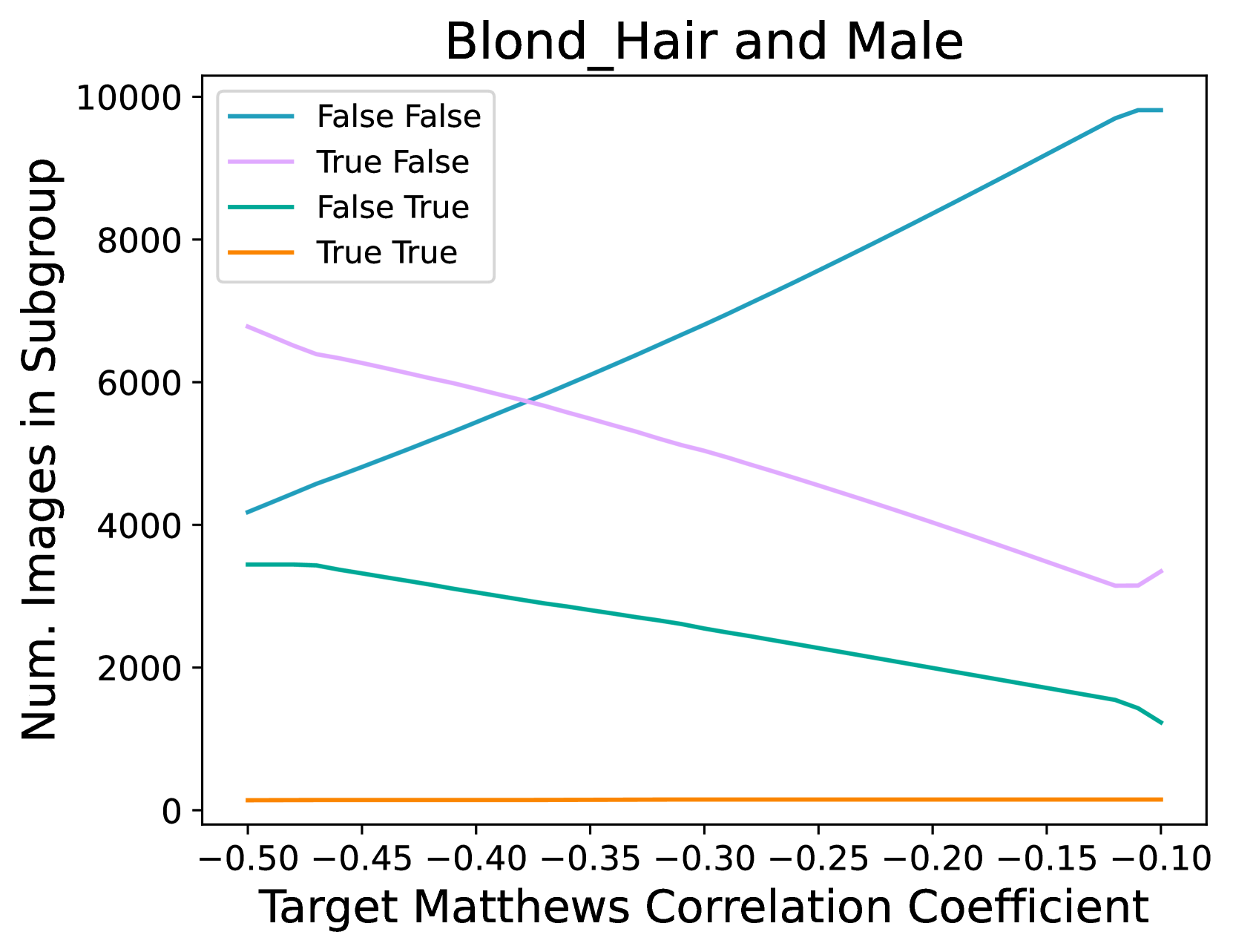
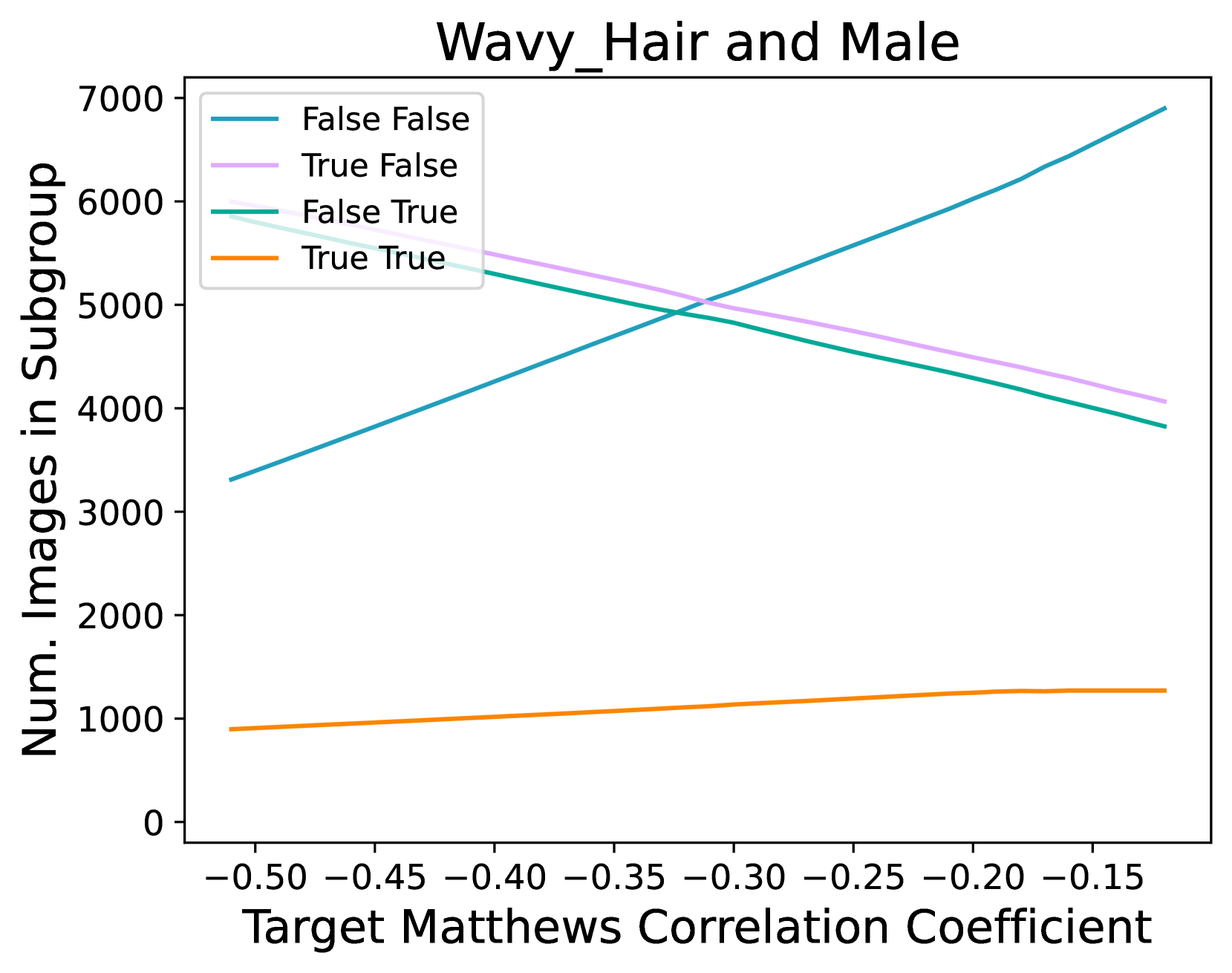
🔼 This figure shows the results of an experiment where the training data was subsampled to vary the correlation between attributes. Specifically, it shows how the sizes of four subgroups (Blond Hair and Male, Wavy Hair and Male) changed to achieve target Matthews Correlation Coefficients (MCCs) between the target attribute and Male. The sizes were constrained to be no smaller than the smallest subsampled training set found during the optimization process. The plot illustrates the relationship between the target MCC and the number of images in each subgroup, providing insights into how manipulating correlations between attributes in the training dataset affects the model’s behavior.
read the caption
Figure 10: Training set subgroup sizes under subsampling. Here we report subgroup sizes of the training set of varying MCCs for Blond_Hair and Wavy_Hair with Male, under our optimization scheme, to compute the results in Sec. 5.2 and Fig. 9. Subgroup sizes are bounded to the smallest subsampled training set size. The legend shows the four different subgroups groups, with the first value indicating the target label and the second Male.
Full paper#
