TL;DR#
Estimating motion is key for computer vision, but current methods often use synthetic data or hand-tuned rules, limiting their real-world use. Recent self-supervised learning offers promise but hasn’t been fully used for motion estimation. Addressing this gap, this paper presents a new approach, leveraging counterfactual probes with pre-trained video models to achieve state-of-the-art motion estimation without using labels.
The paper introduces Opt-CWM, where the core idea involves learning to optimize ‘counterfactual probes’ that extract motion information from a video model. Instead of relying on fixed heuristics or synthetic data, Opt-CWM learns perturbations tailored to the local appearance of the scene. By training a perturbation generator and using it in conjunction with a flow-conditioned predictor, the method achieves impressive results on real-world benchmarks.
Key Takeaways#
Why does it matter?#
This work introduces a novel self-supervised learning method for motion estimation, achieving state-of-the-art results on real-world datasets. It paves the way for more robust and generalizable motion understanding in various applications.
Visual Insights#

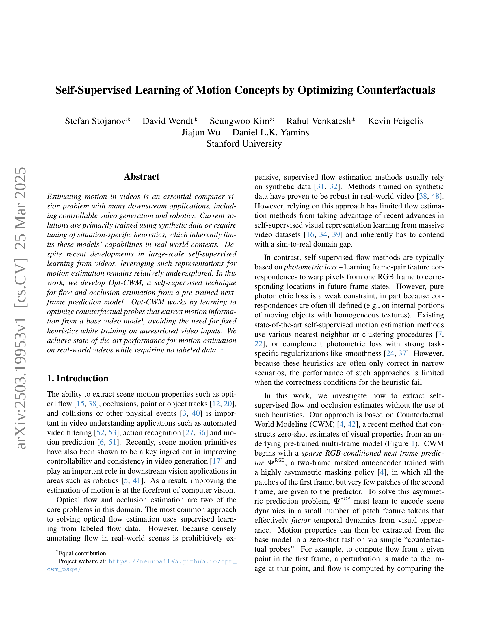
🔼 This figure illustrates the process of extracting optical flow and occlusion information using counterfactual perturbations within the context of Counterfactual World Modeling (CWM). Panel (A) introduces the core concept of CWM, where a model learns to predict the next frame of a video sequence based on a sparsely masked input. The asymmetry in masking the frames enforces the model to learn temporal dynamics efficiently. Panel (B) describes how to estimate optical flow by using a ‘FLOW’ probe. This probe involves applying a local perturbation to a specific point in the first frame and comparing the model’s prediction of the next frame with and without the perturbation. The difference between these two predictions reveals the estimated motion of that point. Finally, panel (C) explains how to estimate occlusion using a similar probe named ‘OCC’. If the resulting difference image is diffuse and has low magnitude, it suggests that the point has been occluded in the following frame.
read the caption
Figure 1: Extracting flow and occlusion with counterfactual perturbation: (A) CWMs learn to predict the next frame with a temporally factored masking policy [4]. (B) The motion of a point can be estimated using a simple counterfactual probing program FLOW: the model predicts the next frame with and without a local perturbation placed on the point, and the difference image between the clean and perturbed predictions reveals the estimated motion. (C) Occlusion is estimated using a related probe OCC: when the perturbation difference image is diffuse and low magnitude, that indicates the perturbed point has been occluded.
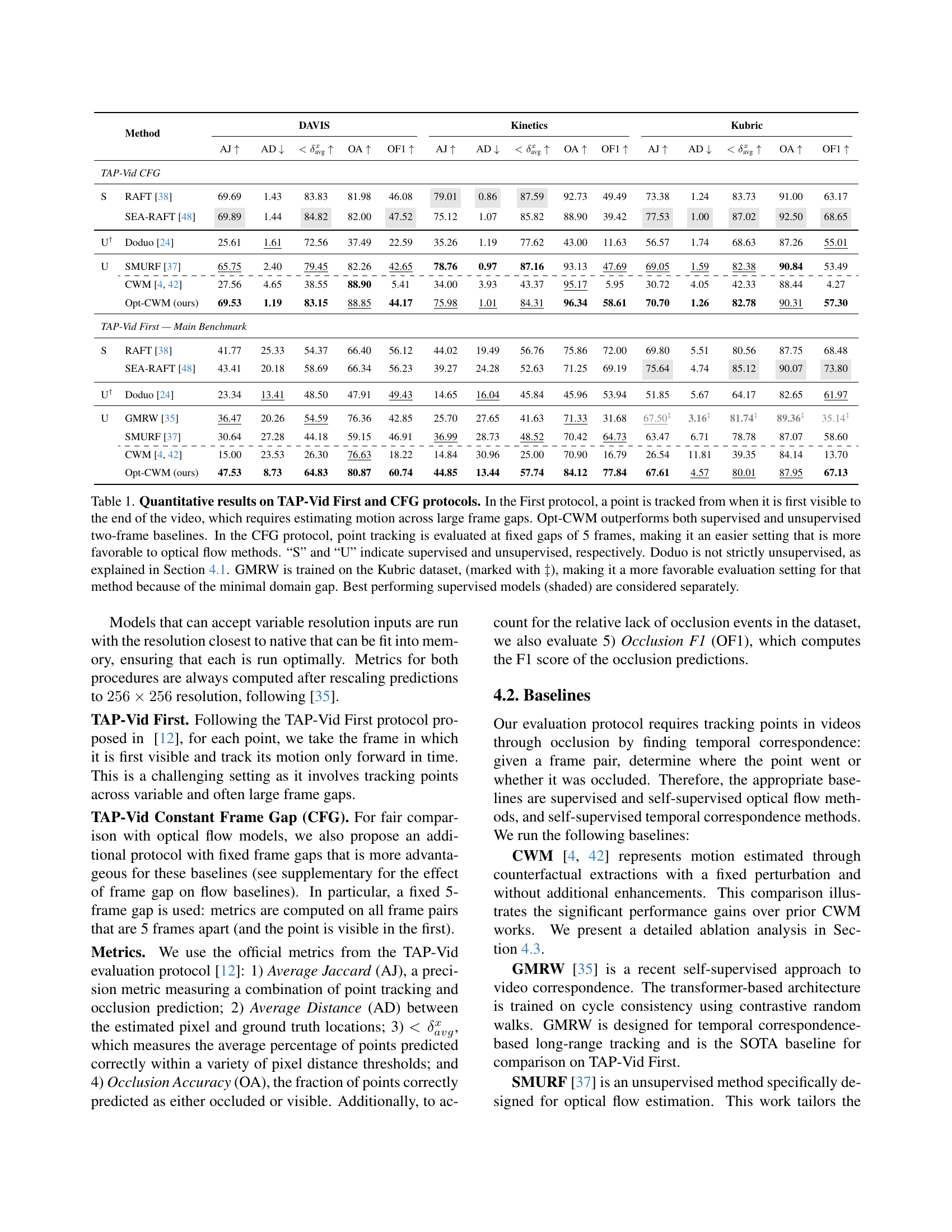
| Method | DAVIS | Kinetics | Kubric | |||||||||||||
| AJ | AD | OA | OF1 | AJ | AD | OA | OF1 | AJ | AD | OA | OF1 | |||||
| TAP-Vid CFG | ||||||||||||||||
| S | RAFT [38] | 69.69 | 1.43 | 83.83 | 81.98 | 46.08 | 79.01 | 0.86 | 87.59 | 92.73 | 49.49 | 73.38 | 1.24 | 83.73 | 91.00 | 63.17 |
| SEA-RAFT [48] | 69.89 | 1.44 | 84.82 | 82.00 | 47.52 | 75.12 | 1.07 | 85.82 | 88.90 | 39.42 | 77.53 | 1.00 | 87.02 | 92.50 | 68.65 | |
| U† | Doduo [24] | 25.61 | 1.61 | 72.56 | 37.49 | 22.59 | 35.26 | 1.19 | 77.62 | 43.00 | 11.63 | 56.57 | 1.74 | 68.63 | 87.26 | 55.01 |
| U | SMURF [37] | 65.75 | 2.40 | 79.45 | 82.26 | 42.65 | 78.76 | 0.97 | 87.16 | 93.13 | 47.69 | 69.05 | 1.59 | 82.38 | 90.84 | 53.49 |
| \cdashline2-17 | CWM [4, 42] | 27.56 | 4.65 | 38.55 | 88.90 | 5.41 | 34.00 | 3.93 | 43.37 | 95.17 | 5.95 | 30.72 | 4.05 | 42.33 | 88.44 | 4.27 |
| Opt-CWM (ours) | 69.53 | 1.19 | 83.15 | 88.85 | 44.17 | 75.98 | 1.01 | 84.31 | 96.34 | 58.61 | 70.70 | 1.26 | 82.78 | 90.31 | 57.30 | |
| TAP-Vid First — Main Benchmark | ||||||||||||||||
| S | RAFT [38] | 41.77 | 25.33 | 54.37 | 66.40 | 56.12 | 44.02 | 19.49 | 56.76 | 75.86 | 72.00 | 69.80 | 5.51 | 80.56 | 87.75 | 68.48 |
| SEA-RAFT [48] | 43.41 | 20.18 | 58.69 | 66.34 | 56.23 | 39.27 | 24.28 | 52.63 | 71.25 | 69.19 | 75.64 | 4.74 | 85.12 | 90.07 | 73.80 | |
| U† | Doduo [24] | 23.34 | 13.41 | 48.50 | 47.91 | 49.43 | 14.65 | 16.04 | 45.84 | 45.96 | 53.94 | 51.85 | 5.67 | 64.17 | 82.65 | 61.97 |
| U | GMRW [35] | 36.47 | 20.26 | 54.59 | 76.36 | 42.85 | 25.70 | 27.65 | 41.63 | 71.33 | 31.68 | 67.50‡ | 3.16‡ | 81.74‡ | 89.36‡ | 35.14‡ |
| SMURF [37] | 30.64 | 27.28 | 44.18 | 59.15 | 46.91 | 36.99 | 28.73 | 48.52 | 70.42 | 64.73 | 63.47 | 6.71 | 78.78 | 87.07 | 58.60 | |
| \cdashline2-17 | CWM [4, 42] | 15.00 | 23.53 | 26.30 | 76.63 | 18.22 | 14.84 | 30.96 | 25.00 | 70.90 | 16.79 | 26.54 | 11.81 | 39.35 | 84.14 | 13.70 |
| Opt-CWM (ours) | 47.53 | 8.73 | 64.83 | 80.87 | 60.74 | 44.85 | 13.44 | 57.74 | 84.12 | 77.84 | 67.61 | 4.57 | 80.01 | 87.95 | 67.13 | |
🔼 Table 1 presents a comparison of different methods for motion estimation, evaluated using two protocols from the TAP-Vid benchmark: First and CFG. The First protocol assesses the ability to track a point from its first appearance to the end of a video, involving significant temporal gaps. The CFG protocol uses fixed 5-frame gaps, which is more advantageous to optical flow techniques. The table shows results for several methods, categorized as supervised (S) or unsupervised (U), indicating how well each method performs on the two protocols, measured by several metrics. Note that Doduo uses some supervised information and GMRW was trained using the Kubric dataset, which introduces a bias.
read the caption
Table 1: Quantitative results on TAP-Vid First and CFG protocols. In the First protocol, a point is tracked from when it is first visible to the end of the video, which requires estimating motion across large frame gaps. Opt-CWM outperforms both supervised and unsupervised two-frame baselines. In the CFG protocol, point tracking is evaluated at fixed gaps of 5 frames, making it an easier setting that is more favorable to optical flow methods. “S” and “U” indicate supervised and unsupervised, respectively. Doduo is not strictly unsupervised, as explained in Section 4.1. GMRW is trained on the Kubric dataset, (marked with ‡‡\ddagger‡), making it a more favorable evaluation setting for that method because of the minimal domain gap. Best performing supervised models (shaded) are considered separately.
In-depth insights#
CWM’s Limitations#
CWM’s hand-designed perturbations present a key limitation. Since the perturbations are fixed, they might be out-of-domain in real-world videos, hindering accurate motion extraction. These perturbations might not properly ‘carry along’ with moving objects, leading to suboptimal counterfactual motion estimation. The fixed nature limits adaptability to complex dynamics. CWM may struggle with deformable objects or scenes with large occlusions because the hard-coded nature doesn’t handle the diversity. Performance is capped by the quality of these static probes. CWM would benefit from learning adaptive perturbations tailored to each scene and its motion dynamics.
Opt-CWM: Innovation#
Opt-CWM innovates by introducing a learnable perturbation generator, moving beyond fixed, hand-designed perturbations in prior Counterfactual World Modeling (CWM). This allows for context-specific motion extraction, where perturbations adapt to local image appearance for more accurate tracking. Crucially, Opt-CWM uses a self-supervised learning approach to train the perturbation generator, eliminating the need for labeled data or heuristics. By coupling a flow-conditioned predictor with the perturbation generator and optimizing for RGB reconstruction, Opt-CWM achieves state-of-the-art motion estimation, showing the power of adaptable, self-learned counterfactual probes.
No Labeled Data#
The concept of learning without labeled data is pivotal. Traditional supervised learning relies heavily on annotated datasets, which are often expensive and time-consuming to create. Eliminating this dependency unlocks the potential to leverage vast amounts of readily available, unlabeled video data. Methods like self-supervision become crucial, where the data provides its own supervisory signals. The focus shifts to designing pretext tasks that enable the model to learn meaningful representations from unlabeled data. Successfully learning without labels allows for greater adaptability to new environments and scenarios where labeled data is scarce or non-existent. This signifies a move towards more generalizable and robust AI systems, capable of understanding and interacting with the world with minimal human intervention. It’s about creating algorithms that inherently find patterns and structures, extracting motion information without needing explicit instructions, leading to greater autonomy.
Outperforms SOTA#
The claim of “outperforming state-of-the-art” (SOTA) is a strong assertion that requires careful consideration. A deep dive would examine the specific benchmarks used. Are these standard datasets widely recognized in the field, or were they custom-built? If custom, their representativeness of real-world scenarios needs scrutiny. Furthermore, the magnitude of improvement matters. A marginal gain might not justify the complexity of a new approach. It’s important to look at statistical significance to rule out random chance. Another crucial factor is generalizability. Does the method shine only on certain data subsets or does it consistently deliver superior results across diverse conditions? The analysis would also look at the computational cost and efficiency. A SOTA method isn’t valuable if it’s too slow or resource-intensive for practical applications. Finally, a truly groundbreaking advance often lies not just in surpassing existing benchmarks, but in opening new avenues for research and practical applications.
Future Extraction#
Future extraction in self-supervised learning of motion can revolve around several key aspects. Firstly, scaling the approach to handle longer video sequences and more complex scenes remains a key challenge, this necessitates exploring efficient architectures and training techniques. Secondly, extending the framework to extract a broader range of visual properties beyond motion, such as object segments, depth maps, and 3D shape, presents a promising avenue for future research. Thirdly, exploring different base predictor architectures, such as auto-regressive generative models, could lead to improved performance and capabilities. Lastly, the twin techniques of parameterizing the input-conditioned counterfactual generator and bootstrapping the learning of the generator parameters with end-to-end sparse prediction loss are generic and not flow-specific and may thus be extensible to optimizing highly performant CWM-style extraction.
More visual insights#
More on figures

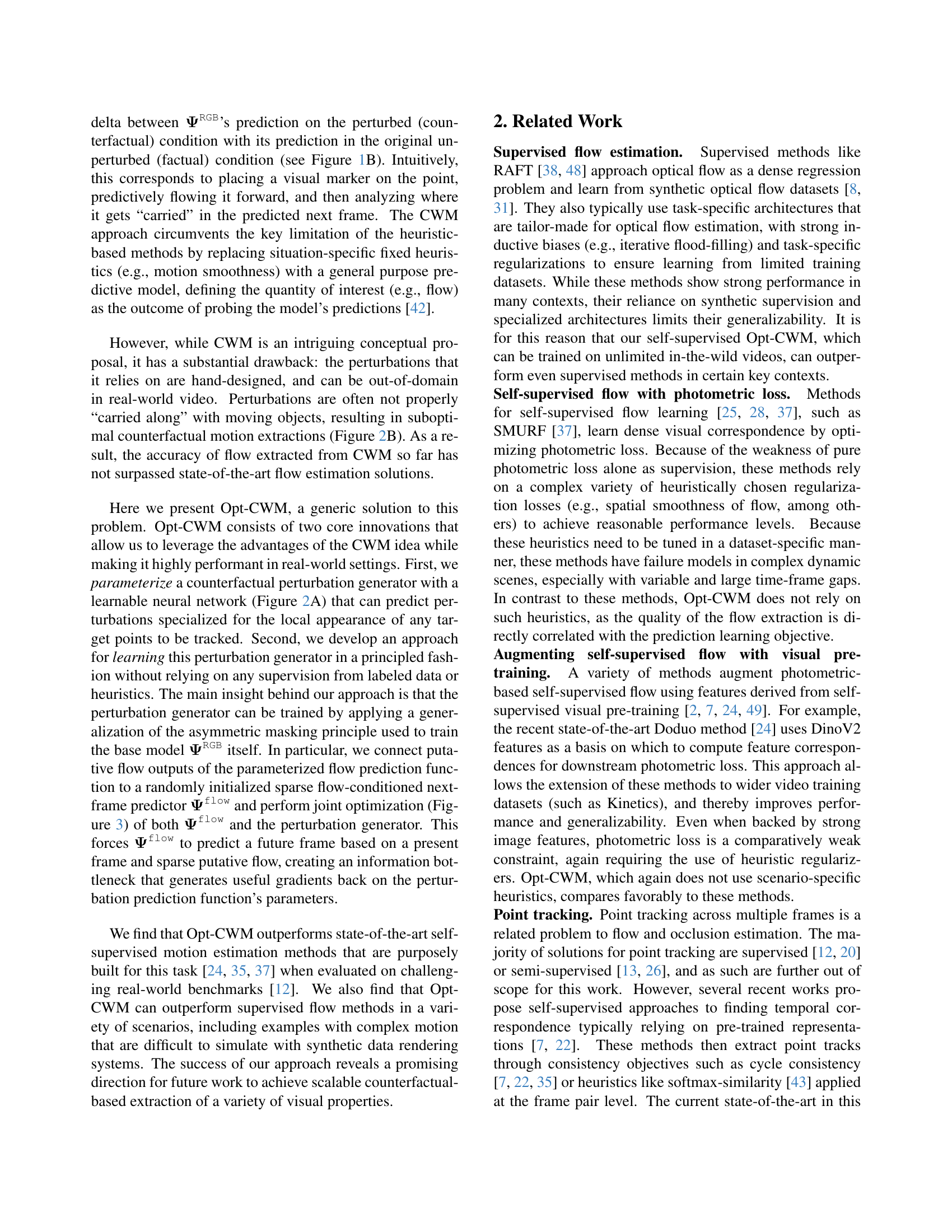
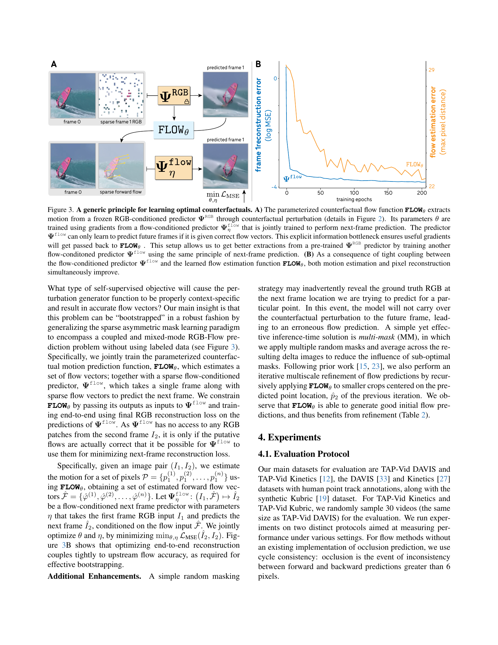
🔼 This figure illustrates how the Opt-CWM model parameterizes counterfactual perturbations to improve motion estimation. Panel (A) shows the architecture, where a learned perturbation generator (δθ) is added to a pre-trained next-frame prediction model (ΨRGB). This generator uses an MLP to predict perturbations based on image content. Panel (B) contrasts hand-designed perturbations, which often fail to move consistently with objects, against learned perturbations, which integrate more seamlessly with the scene dynamics. This shows how the learnable perturbation generator addresses limitations of hand-designed methods. The caption asks how to learn the parameters of the perturbation generator without labeled data, which is answered in Figure 3.
read the caption
Figure 2: Parameterizing the counterfactual intervention policy as an input-conditioned function. (A) Building on a pre-trained RGB-conditioned predictor 𝚿RGBsuperscript𝚿RGB\boldsymbol{\Psi}^{\texttt{RGB}}bold_Ψ start_POSTSUPERSCRIPT RGB end_POSTSUPERSCRIPT, Opt-CWM uses an image-conditioned perturbation prediction function δθsubscript𝛿𝜃\delta_{\theta}italic_δ start_POSTSUBSCRIPT italic_θ end_POSTSUBSCRIPT containing a small MLPθ. As illustrated in B, δθsubscript𝛿𝜃\delta_{\theta}italic_δ start_POSTSUBSCRIPT italic_θ end_POSTSUBSCRIPT can learn to predict image-conditioned perturbations that blend naturally with the underlying scene, potentially allowing for the perturbation to be accurately carried over to the next frame prediction. But how should the parameters of δθsubscript𝛿𝜃\delta_{\theta}italic_δ start_POSTSUBSCRIPT italic_θ end_POSTSUBSCRIPT be learned to achieve this, without any flow supervision labels? See Figure 3.

🔼 Figure 3 illustrates the training process of the Opt-CWM model. Panel A shows the architecture: a pre-trained RGB-conditioned next-frame predictor (ΨRGB) is used as a base model. A learnable counterfactual perturbation generator (FLOWθ) creates perturbations, which are applied to the input frame before feeding it to ΨRGB. The output of ΨRGB is compared with the prediction without perturbation. This difference provides information about motion, which is used to train a flow-conditioned next-frame predictor (Ψflowη). The latter model learns to predict the next frame based on both the original frame and the sparse flow information (which necessitates accurate flow estimates from FLOWθ). Panel B shows how the reconstruction and flow estimation errors change during training. The tight coupling between the two models ensures that improvements in motion estimation directly benefit frame reconstruction, and vice-versa.
read the caption
Figure 3: A generic principle for learning optimal counterfactuals. A) The parameterized counterfactual flow function FLOWθsubscriptFLOW𝜃\textbf{{FLOW}}_{\theta}FLOW start_POSTSUBSCRIPT italic_θ end_POSTSUBSCRIPT extracts motion from a frozen RGB-conditioned predictor 𝚿RGBsuperscript𝚿RGB\boldsymbol{\Psi}^{\texttt{RGB}}bold_Ψ start_POSTSUPERSCRIPT RGB end_POSTSUPERSCRIPT through counterfactual perturbation (details in Figure 2). Its parameters θ𝜃\thetaitalic_θ are trained using gradients from a flow-conditioned predictor 𝚿ηflowsubscriptsuperscript𝚿flow𝜂\boldsymbol{\Psi}^{\texttt{flow}}_{\eta}bold_Ψ start_POSTSUPERSCRIPT flow end_POSTSUPERSCRIPT start_POSTSUBSCRIPT italic_η end_POSTSUBSCRIPT that is jointly trained to perform next-frame prediction. The predictor 𝚿flowsuperscript𝚿flow\boldsymbol{\Psi}^{\texttt{flow}}bold_Ψ start_POSTSUPERSCRIPT flow end_POSTSUPERSCRIPT can only learn to predict future frames if it is given correct flow vectors. This explicit information bottleneck ensures useful gradients will get passed back to FLOWθsubscriptFLOW𝜃\textbf{{FLOW}}_{\theta}FLOW start_POSTSUBSCRIPT italic_θ end_POSTSUBSCRIPT . This setup allows us to get better extractions from a pre-trained 𝚿RGBsuperscript𝚿RGB\boldsymbol{\Psi}^{\texttt{RGB}}bold_Ψ start_POSTSUPERSCRIPT RGB end_POSTSUPERSCRIPT predictor by training another flow-conditoned predictor 𝚿flowsuperscript𝚿flow\boldsymbol{\Psi}^{\texttt{flow}}bold_Ψ start_POSTSUPERSCRIPT flow end_POSTSUPERSCRIPT using the same principle of next-frame prediction. (B) As a consequence of tight coupling between the flow-conditioned predictor 𝚿flowsuperscript𝚿flow\boldsymbol{\Psi}^{\texttt{flow}}bold_Ψ start_POSTSUPERSCRIPT flow end_POSTSUPERSCRIPT and the learned flow estimation function FLOWθsubscriptFLOW𝜃\textbf{{FLOW}}_{\theta}FLOW start_POSTSUBSCRIPT italic_θ end_POSTSUBSCRIPT, both motion estimation and pixel reconstruction simultaneously improve.

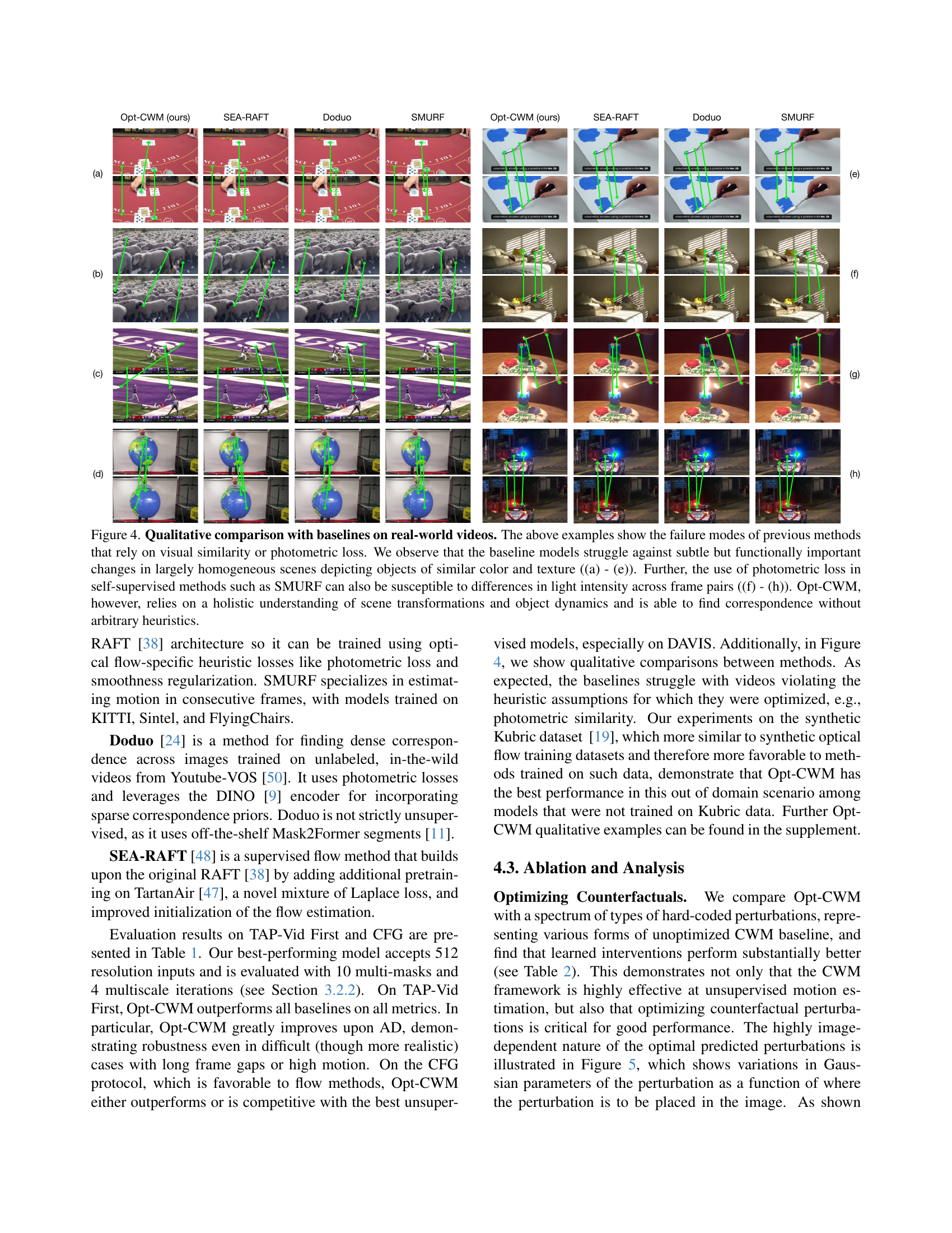
🔼 This figure showcases a qualitative comparison of Opt-CWM’s performance against other state-of-the-art methods on real-world video sequences. The examples highlight scenarios where methods relying on visual similarity or photometric loss fail. Specifically, it demonstrates that baselines struggle with subtle but significant changes within homogeneous scenes, particularly when objects share similar colors and textures (examples (a) through (e)). It also demonstrates the vulnerability of photometric loss-based methods, like SMURF, to variations in light intensity between frames (examples (f) through (h)). In contrast, Opt-CWM, due to its holistic approach which considers scene transformations and dynamics, consistently achieves superior performance in these challenging situations.
read the caption
Figure 4: Qualitative comparison with baselines on real-world videos. The above examples show the failure modes of previous methods that rely on visual similarity or photometric loss. We observe that the baseline models struggle against subtle but functionally important changes in largely homogeneous scenes depicting objects of similar color and texture ((a) - (e)). Further, the use of photometric loss in self-supervised methods such as SMURF can also be susceptible to differences in light intensity across frame pairs ((f) - (h)). Opt-CWM, however, relies on a holistic understanding of scene transformations and object dynamics and is able to find correspondence without arbitrary heuristics.

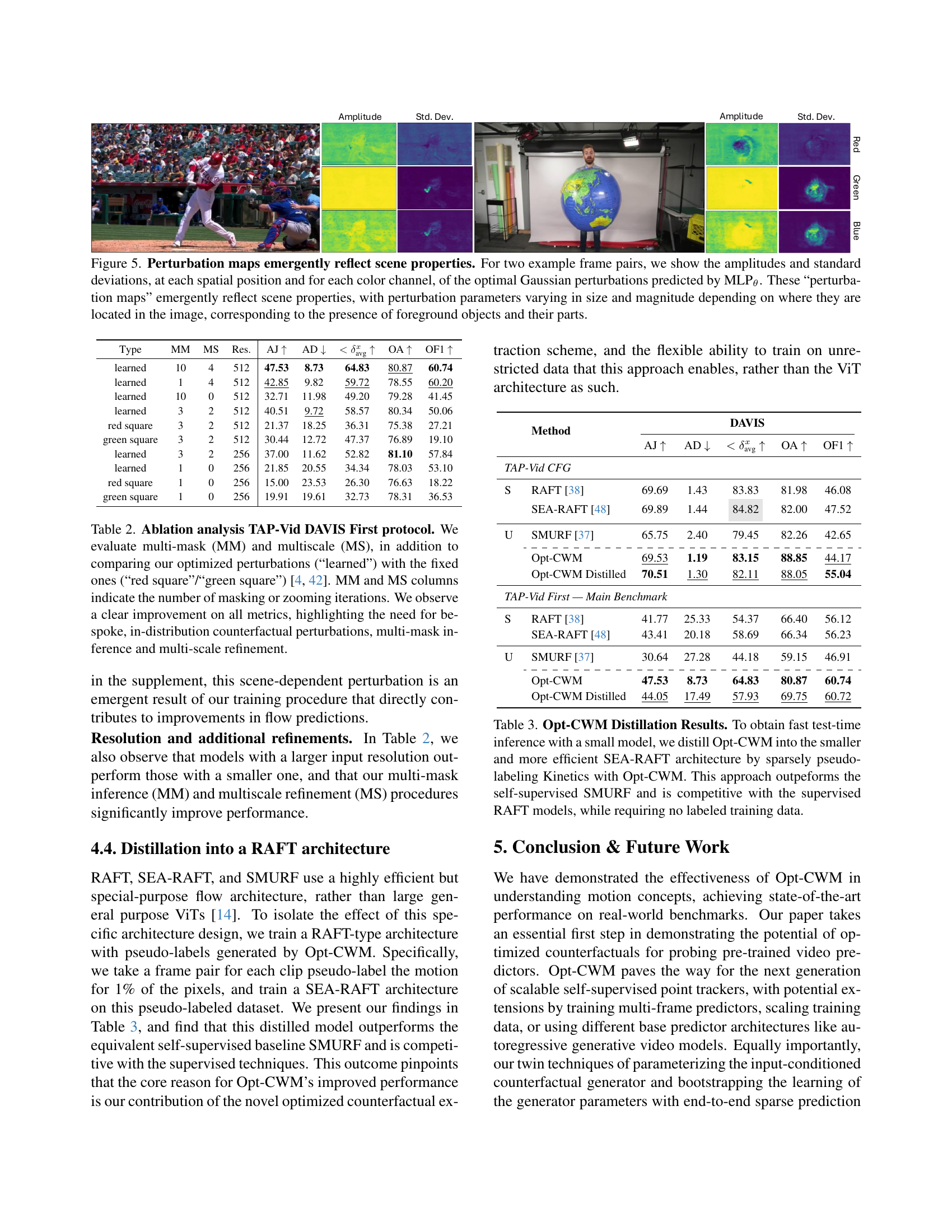
🔼 This figure visualizes learned perturbation maps generated by a learned MLP (Multilayer Perceptron). The maps show the amplitudes and standard deviations of optimal Gaussian perturbations predicted for each pixel location and color channel across two example frame pairs. The size and magnitude of these perturbations dynamically adapt to local scene content. Specifically, they reflect the presence and characteristics of foreground objects. The perturbations are not uniform but are shaped to match features of the image, suggesting the model has learned to represent scene properties within them.
read the caption
Figure 5: Perturbation maps emergently reflect scene properties. For two example frame pairs, we show the amplitudes and standard deviations, at each spatial position and for each color channel, of the optimal Gaussian perturbations predicted by MLPθ. These “perturbation maps” emergently reflect scene properties, with perturbation parameters varying in size and magnitude depending on where they are located in the image, corresponding to the presence of foreground objects and their parts.

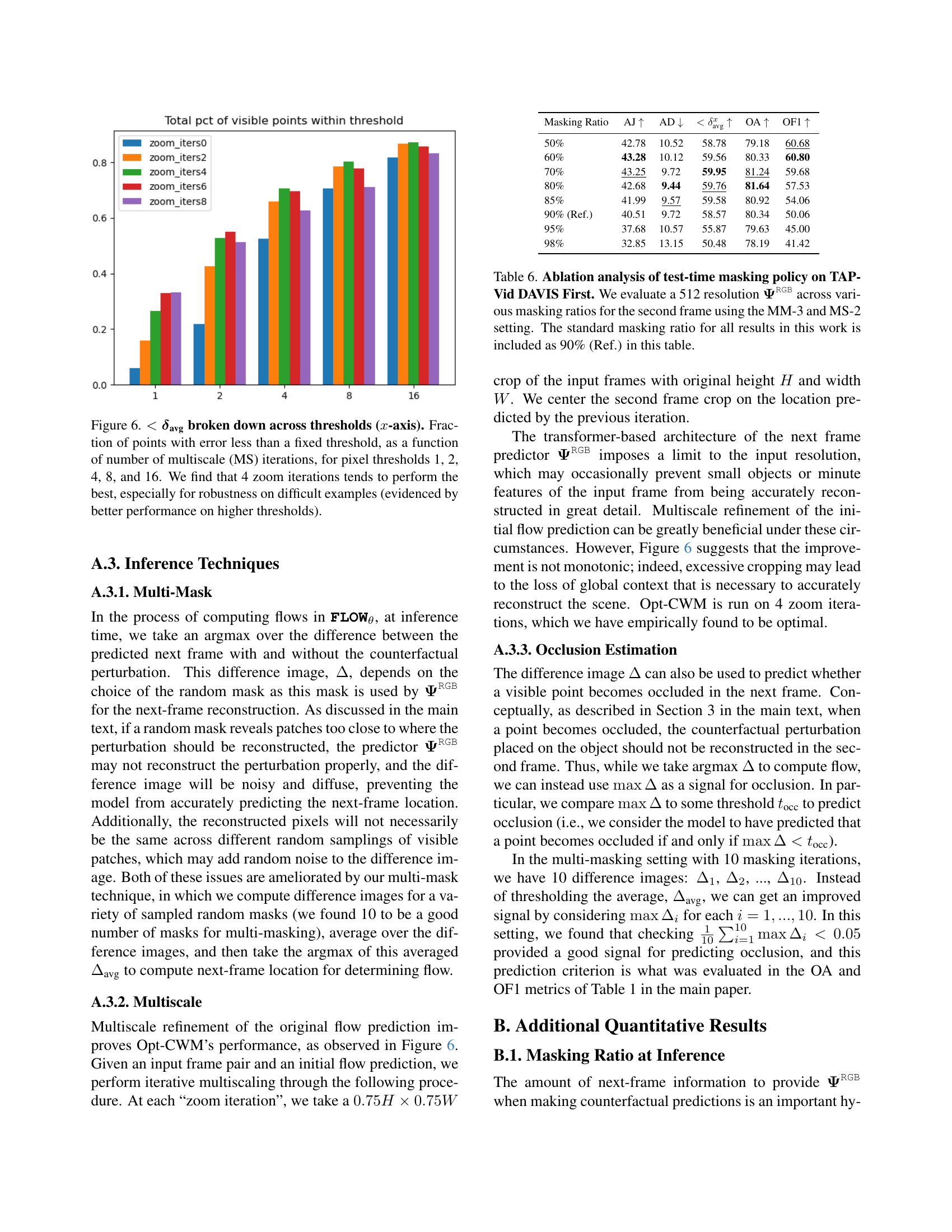
🔼 This figure analyzes the impact of multiscale refinement on the accuracy of flow estimation. The x-axis represents different pixel error thresholds, while the y-axis shows the fraction of points whose error is below each threshold. Different colored bars represent varying numbers of multiscale iterations. The results indicate that 4 zoom iterations provide the best performance overall, particularly when dealing with challenging cases (as demonstrated by its better performance at higher error thresholds).
read the caption
Figure 6: <𝜹avgabsentsubscript𝜹avg<\boldsymbol{\delta}_{\text{avg}}< bold_italic_δ start_POSTSUBSCRIPT avg end_POSTSUBSCRIPT broken down across thresholds (x𝑥xitalic_x-axis). Fraction of points with error less than a fixed threshold, as a function of number of multiscale (MS) iterations, for pixel thresholds 1, 2, 4, 8, and 16. We find that 4 zoom iterations tends to perform the best, especially for robustness on difficult examples (evidenced by better performance on higher thresholds).

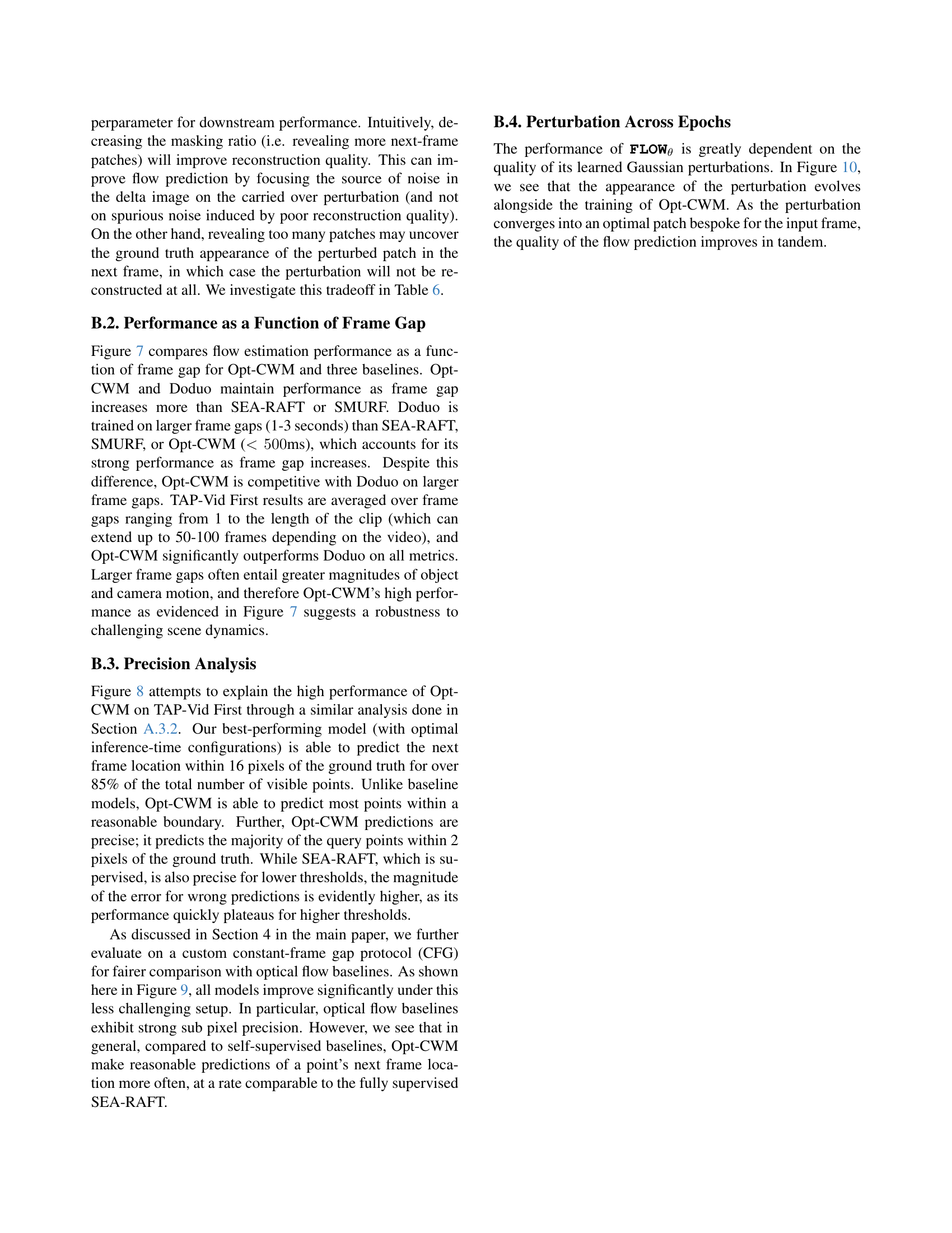
🔼 This figure compares the performance of various optical flow estimation methods (Opt-CWM, Doduo, SEA-RAFT, and SMURF) as the gap between frames increases. The x-axis represents the frame gap, while the y-axis shows the average pixel distance (AD) error, a key metric of accuracy. The results reveal that Opt-CWM and Doduo maintain relatively high accuracy even with larger frame gaps, unlike SEA-RAFT and SMURF, whose accuracy significantly decreases as the frame gap and motion magnitude increase. This suggests that Opt-CWM and Doduo are more robust to challenging real-world scenarios with substantial motion between frames.
read the caption
Figure 7: Model comparison as a function of frame gap. Higher frame gaps present harder flow estimation problems due to including more motion, as reflected by improved performance across models in lower frame gap settings. Opt-CWM and Doduo perform better as frame gap increases, in contrast to optical flow methods SEA-RAFT and SMURF which decay in performance as motion magnitude increases, especially on the AD metric.

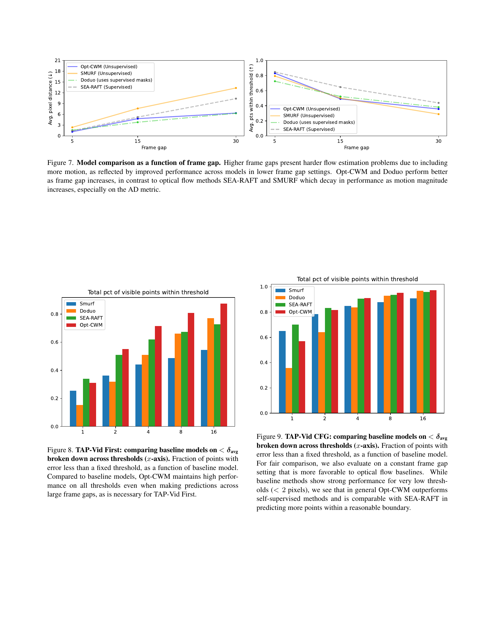
🔼 Figure 8 presents a detailed analysis of the accuracy of different models in predicting the location of points across various error thresholds. The x-axis represents the error threshold (in pixels), while the y-axis shows the percentage of points for which the predicted location falls within that threshold of the ground truth. The graph compares Opt-CWM with three baseline models: SEA-RAFT, Doduo, and SMURF. Importantly, the evaluation considers videos with large gaps between frames (the TAP-Vid First protocol), making accurate point tracking particularly challenging. The results demonstrate that Opt-CWM consistently achieves higher accuracy across all error thresholds, particularly for larger thresholds. This highlights the robustness of Opt-CWM in handling scenarios with significant motion and longer frame intervals, which cause challenges for other methods.
read the caption
Figure 8: TAP-Vid First: comparing baseline models on <δavgabsentsubscript𝛿avg<\boldsymbol{\delta}_{\text{avg}}< bold_italic_δ start_POSTSUBSCRIPT avg end_POSTSUBSCRIPT broken down across thresholds (x𝑥xitalic_x-axis). Fraction of points with error less than a fixed threshold, as a function of baseline model. Compared to baseline models, Opt-CWM maintains high performance on all thresholds even when making predictions across large frame gaps, as is necessary for TAP-Vid First.

🔼 Figure 9 presents a comparative analysis of various models’ performance on the TAP-Vid CFG (Constant Frame Gap) benchmark, focusing on the average point tracking error. The x-axis represents different error thresholds (in pixels), and the y-axis shows the percentage of points whose error falls below each threshold. The dataset uses a fixed frame gap, making it advantageous for optical flow methods. While supervised and unsupervised optical flow methods perform well at very low error thresholds (under 2 pixels), Opt-CWM demonstrates superior performance overall, outperforming self-supervised approaches and achieving comparable results to the supervised SEA-RAFT method in predicting a higher proportion of points within an acceptable error range.
read the caption
Figure 9: TAP-Vid CFG: comparing baseline models on <δavgabsentsubscript𝛿avg<\boldsymbol{\delta}_{\text{avg}}< bold_italic_δ start_POSTSUBSCRIPT avg end_POSTSUBSCRIPT broken down across thresholds (x𝑥xitalic_x-axis). Fraction of points with error less than a fixed threshold, as a function of baseline model. For fair comparison, we also evaluate on a constant frame gap setting that is more favorable to optical flow baselines. While baseline methods show strong performance for very low thresholds (<2absent2<2< 2 pixels), we see that in general Opt-CWM outperforms self-supervised methods and is comparable with SEA-RAFT in predicting more points within a reasonable boundary.

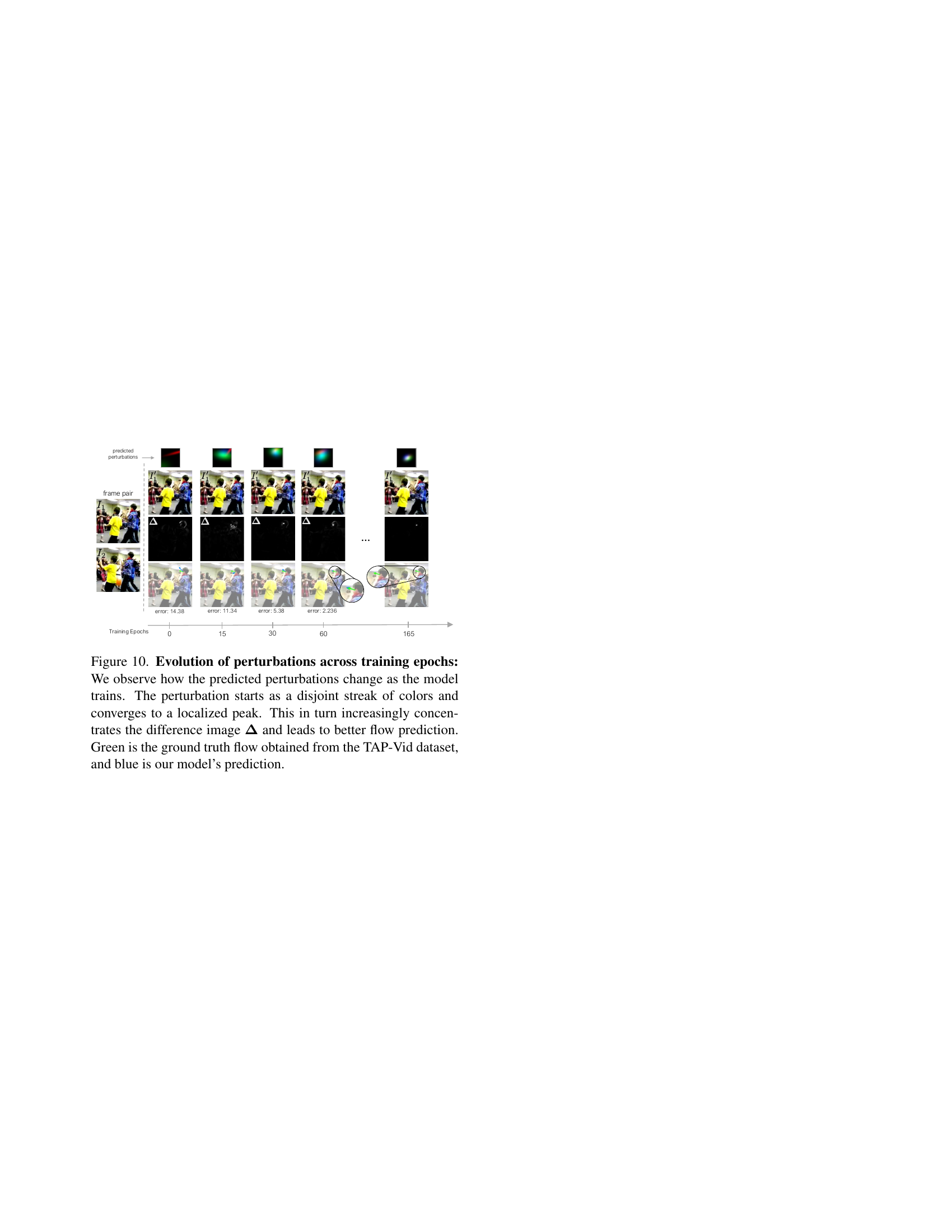
🔼 This figure visualizes the evolution of learned perturbations throughout the training process of the Opt-CWM model. It shows how the model’s ability to generate effective perturbations improves over time. Initially, the perturbations are scattered and lack coherence. As training progresses, these perturbations become more concentrated and localized, improving the accuracy of the resulting flow predictions. The figure demonstrates this by showing example perturbation maps at various training epochs alongside a comparison of the ground truth flow (green) from the TAP-Vid dataset and the Opt-CWM model’s predicted flow (blue) for those same examples. The decreasing error between the ground truth flow and the model’s prediction, as demonstrated by the diminishing numerical error value shown, is directly correlated to the evolution of the perturbation.
read the caption
Figure 10: Evolution of perturbations across training epochs: We observe how the predicted perturbations change as the model trains. The perturbation starts as a disjoint streak of colors and converges to a localized peak. This in turn increasingly concentrates the difference image 𝚫𝚫\boldsymbol{\Delta}bold_Δ and leads to better flow prediction. Green is the ground truth flow obtained from the TAP-Vid dataset, and blue is our model’s prediction.
More on tables
| Type | MM | MS | Res. | AJ | AD | OA | OF1 | |
| learned | 10 | 4 | 512 | 47.53 | 8.73 | 64.83 | 80.87 | 60.74 |
| learned | 1 | 4 | 512 | 42.85 | 9.82 | 59.72 | 78.55 | 60.20 |
| learned | 10 | 0 | 512 | 32.71 | 11.98 | 49.20 | 79.28 | 41.45 |
| learned | 3 | 2 | 512 | 40.51 | 9.72 | 58.57 | 80.34 | 50.06 |
| red square | 3 | 2 | 512 | 21.37 | 18.25 | 36.31 | 75.38 | 27.21 |
| green square | 3 | 2 | 512 | 30.44 | 12.72 | 47.37 | 76.89 | 19.10 |
| learned | 3 | 2 | 256 | 37.00 | 11.62 | 52.82 | 81.10 | 57.84 |
| learned | 1 | 0 | 256 | 21.85 | 20.55 | 34.34 | 78.03 | 53.10 |
| red square | 1 | 0 | 256 | 15.00 | 23.53 | 26.30 | 76.63 | 18.22 |
| green square | 1 | 0 | 256 | 19.91 | 19.61 | 32.73 | 78.31 | 36.53 |
🔼 This table presents an ablation study on the TAP-Vid DAVIS First protocol, evaluating the impact of various design choices on the performance of the Opt-CWM model. The study compares different types of perturbations (hand-designed vs. learned) and techniques such as multi-mask inference and multi-scale refinement. The results, measured across multiple metrics, demonstrate that learned, in-distribution perturbations, coupled with multi-mask inference and multi-scale refinement significantly improve the model’s ability to estimate motion.
read the caption
Table 2: Ablation analysis TAP-Vid DAVIS First protocol. We evaluate multi-mask (MM) and multiscale (MS), in addition to comparing our optimized perturbations (“learned”) with the fixed ones (“red square”/“green square”) [4, 42]. MM and MS columns indicate the number of masking or zooming iterations. We observe a clear improvement on all metrics, highlighting the need for bespoke, in-distribution counterfactual perturbations, multi-mask inference and multi-scale refinement.
| Method | DAVIS | |||||
| AJ | AD | OA | OF1 | |||
| TAP-Vid CFG | ||||||
| S | RAFT [38] | 69.69 | 1.43 | 83.83 | 81.98 | 46.08 |
| SEA-RAFT [48] | 69.89 | 1.44 | 84.82 | 82.00 | 47.52 | |
| U | SMURF [37] | 65.75 | 2.40 | 79.45 | 82.26 | 42.65 |
| \cdashline2-7 | Opt-CWM | 69.53 | 1.19 | 83.15 | 88.85 | 44.17 |
| Opt-CWM Distilled | 70.51 | 1.30 | 82.11 | 88.05 | 55.04 | |
| TAP-Vid First — Main Benchmark | ||||||
| S | RAFT [38] | 41.77 | 25.33 | 54.37 | 66.40 | 56.12 |
| SEA-RAFT [48] | 43.41 | 20.18 | 58.69 | 66.34 | 56.23 | |
| U | SMURF [37] | 30.64 | 27.28 | 44.18 | 59.15 | 46.91 |
| \cdashline2-7 | Opt-CWM | 47.53 | 8.73 | 64.83 | 80.87 | 60.74 |
| Opt-CWM Distilled | 44.05 | 17.49 | 57.93 | 69.75 | 60.72 | |
🔼 This table presents the results of distilling the Opt-CWM model into a smaller, more efficient SEA-RAFT architecture. Instead of using labeled data for training, the researchers used sparsely pseudo-labeled Kinetics data generated by Opt-CWM. The goal was to achieve fast test-time inference while maintaining performance. The results show that this distilled model outperforms the self-supervised SMURF model and is competitive with supervised RAFT models, demonstrating the effectiveness of this approach.
read the caption
Table 3: Opt-CWM Distillation Results. To obtain fast test-time inference with a small model, we distill Opt-CWM into the smaller and more efficient SEA-RAFT architecture by sparsely pseudo-labeling Kinetics with Opt-CWM. This approach outpeforms the self-supervised SMURF and is competitive with the supervised RAFT models, while requiring no labeled training data.
| config | value |
| optimizer | AdamW [30] |
| base learning rate | 1.5e-4 |
| weight decay | 0.05 |
| optimizer momentum | [10] |
| accumulative batch size | 4096 |
| learning rate schedule | cosine decay [29] |
| warmup epochs [18] | 40 |
| total epochs | 800 |
| flip augmentation | no |
| augmentation | MultiScaleCrop [44] |
🔼 This table details the hyperparameters used for pre-training the Counterfactual World Model (CWM) which is a core component of the Opt-CWM model. It shows the optimizer used, learning rate, weight decay, momentum, batch size, learning rate schedule, number of warmup and total training epochs, and data augmentation strategies employed.
read the caption
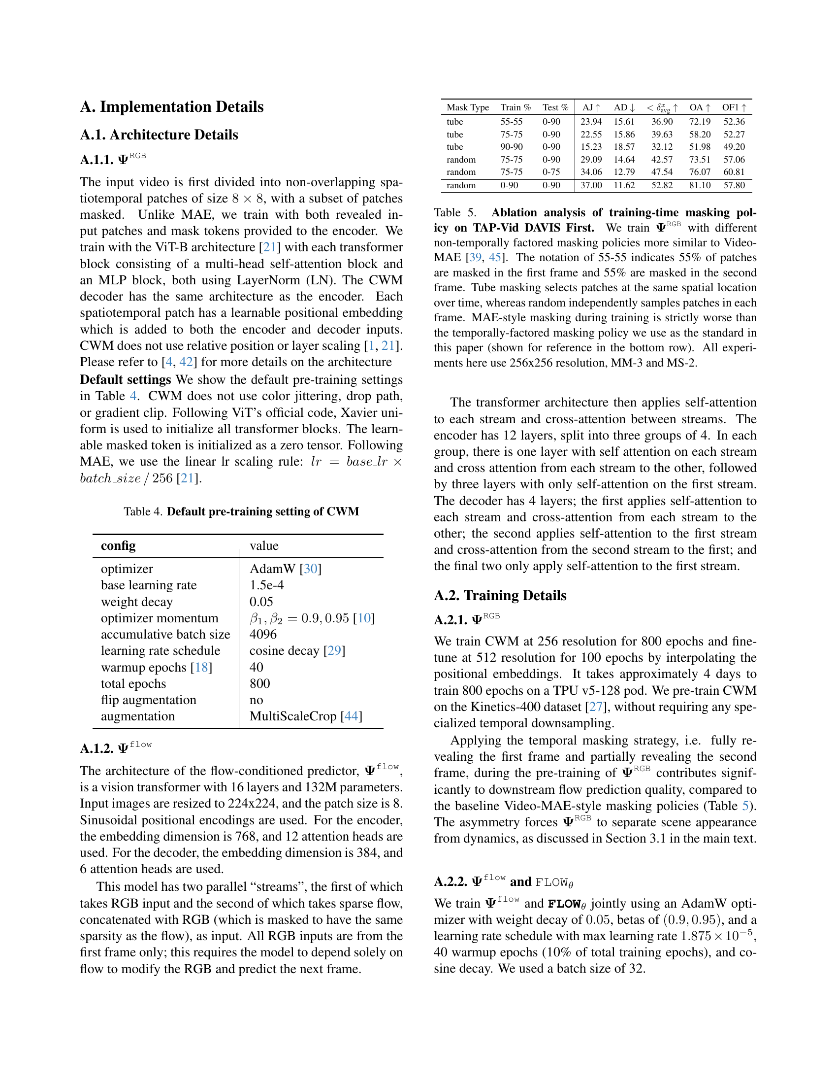
Table 4: Default pre-training setting of CWM
| Mask Type | Train % | Test % | AJ | AD | OA | OF1 | |
| tube | 55-55 | 0-90 | 23.94 | 15.61 | 36.90 | 72.19 | 52.36 |
| tube | 75-75 | 0-90 | 22.55 | 15.86 | 39.63 | 58.20 | 52.27 |
| tube | 90-90 | 0-90 | 15.23 | 18.57 | 32.12 | 51.98 | 49.20 |
| random | 75-75 | 0-90 | 29.09 | 14.64 | 42.57 | 73.51 | 57.06 |
| random | 75-75 | 0-75 | 34.06 | 12.79 | 47.54 | 76.07 | 60.81 |
| random | 0-90 | 0-90 | 37.00 | 11.62 | 52.82 | 81.10 | 57.80 |
🔼 This table presents an ablation study on the impact of different training-time masking policies for the RGB-conditioned next frame predictor (ΨRGB). It compares the performance of various masking strategies, including those similar to Video-MAE, where a percentage of patches are masked in each frame (55-55 means 55% in frame 1 and 55% in frame 2). It also explores ’tube’ masking (masking the same spatial location across frames) and completely random masking. The results are evaluated using the TAP-Vid DAVIS First protocol with 256x256 resolution, 3 multi-mask iterations, and 2 multiscale iterations. The goal is to show the impact of the masking policy on the final motion estimation performance, demonstrating that the temporally factored masking policy used in the main experiments is superior.
read the caption
Table 5: Ablation analysis of training-time masking policy on TAP-Vid DAVIS First. We train 𝚿RGBsuperscript𝚿RGB\boldsymbol{\Psi}^{\texttt{RGB}}bold_Ψ start_POSTSUPERSCRIPT RGB end_POSTSUPERSCRIPT with different non-temporally factored masking policies more similar to Video-MAE [39, 45]. The notation of 55-55 indicates 55% of patches are masked in the first frame and 55% are masked in the second frame. Tube masking selects patches at the same spatial location over time, whereas random independently samples patches in each frame. MAE-style masking during training is strictly worse than the temporally-factored masking policy we use as the standard in this paper (shown for reference in the bottom row). All experiments here use 256x256 resolution, MM-3 and MS-2.
| Masking Ratio | AJ | AD | OA | OF1 | |
| 50% | 42.78 | 10.52 | 58.78 | 79.18 | 60.68 |
| 60% | 43.28 | 10.12 | 59.56 | 80.33 | 60.80 |
| 70% | 43.25 | 9.72 | 59.95 | 81.24 | 59.68 |
| 80% | 42.68 | 9.44 | 59.76 | 81.64 | 57.53 |
| 85% | 41.99 | 9.57 | 59.58 | 80.92 | 54.06 |
| 90% (Ref.) | 40.51 | 9.72 | 58.57 | 80.34 | 50.06 |
| 95% | 37.68 | 10.57 | 55.87 | 79.63 | 45.00 |
| 98% | 32.85 | 13.15 | 50.48 | 78.19 | 41.42 |
🔼 This table presents an ablation study on the test-time masking policy used in the Opt-CWM model. Specifically, it investigates the impact of varying the percentage of masked patches in the second frame (the masking ratio) during the inference phase of the model, while keeping other parameters (such as multi-masking iterations and multi-scale refinement) constant at MM=3 and MS=2. The table shows the performance of the model (measured by Average Jaccard (AJ), Average Distance (AD), average percentage of points predicted correctly within various distance thresholds (< avg), Occlusion Accuracy (OA), and Occlusion F1-score (OF1)) across different masking ratios. A reference masking ratio (90%) used in the main experiments is also included for comparison. The experiment was performed on the TAP-Vid DAVIS First benchmark using a 512-resolution RGB-conditioned next frame predictor.
read the caption
Table 6: Ablation analysis of test-time masking policy on TAP-Vid DAVIS First. We evaluate a 512 resolution 𝚿RGBsuperscript𝚿RGB\boldsymbol{\Psi}^{\texttt{RGB}}bold_Ψ start_POSTSUPERSCRIPT RGB end_POSTSUPERSCRIPT across various masking ratios for the second frame using the MM-3 and MS-2 setting. The standard masking ratio for all results in this work is included as 90% (Ref.) in this table.
Full paper#
