TL;DR#
Recent advancements in 2D and multimodal models have shown success by leveraging large-scale training datasets, but extending these achievements to enable free-form interactions with complex 3D/4D scenes is still challenging due to limited annotated 3D/4D datasets. To address this, the paper introduces Feature4X, a framework to extend any functionality from a 2D vision model into the 4D realm, using only monocular video input and adaptable, model-conditioned 4D feature field distillation.The core of the framework involves a dynamic optimization strategy that unifies multiple model capabilities into a single representation.
Feature4X enhances dynamic 3D Gaussian Splatting with a unified latent feature capable of distilling diverse 2D foundation features for flexibility and efficiency, representing the dense 4D feature field using a sparse set of base features. The method is fully differentiable and uses ground truth color, feature maps from 2D vision models, and an LLM-powered agentic AI to interpret natural language prompts and dynamically adjust parameters for intelligent 4D scene interaction.
Key Takeaways#
Why does it matter?#
Feature4X enables versatile 4D scene understanding from monocular video, bridging the gap between 2D foundation models and agentic AI, offering new possibilities for interactive dynamic scene analysis and manipulation, paving the way for immersive 4D interaction.
Visual Insights#

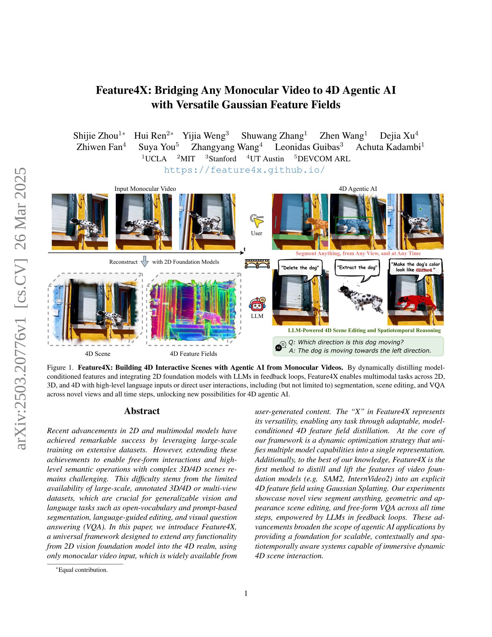
🔼 Figure 1 showcases Feature4X, a framework that generates interactive 4D scenes from monocular videos. It combines model-distilled features, 2D foundation models, and LLMs to enable various tasks such as segmentation, scene editing, and visual question answering (VQA) across different dimensions (2D, 3D, 4D), viewpoints, and timesteps. The user can interact using either high-level language commands or direct manipulations.
read the caption
Figure 1: Feature4X: Building 4D Interactive Scenes with Agentic AI from Monocular Videos. By dynamically distilling model-conditioned features and integrating 2D foundation models with LLMs in feedback loops, Feature4X enables multimodal tasks across 2D, 3D, and 4D with high-level language inputs or direct user interactions, including (but not limited to) segmentation, scene editing, and VQA across novel views and all time steps, unlocking new possibilities for 4D agentic AI.
| Method | PSNR | mIoU | accuracy | Size (MB) |
|---|---|---|---|---|
| MoSca | 25.166 | - | - | 67.726 |
| MoSca + Feature 3DGS | 25.191 | 0.506 | 0.881 | 593.907 |
| Ours (single CLIP head) | 25.186 | 0.510 | 0.880 | 95.294 |
| Ours (full model) | 25.197 | 0.503 | 0.876 | 95.457 |
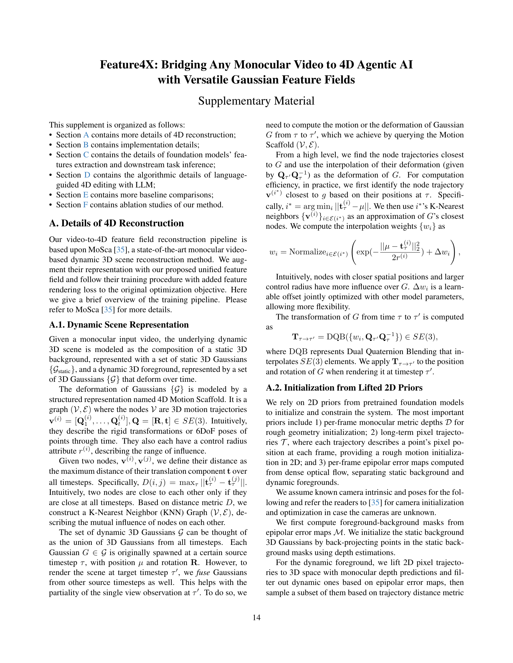
🔼 This table presents a quantitative comparison of semantic segmentation performance on the Nvidia dataset [47] among different methods. The metrics compared include Peak Signal-to-Noise Ratio (PSNR) for radiance reconstruction quality, mean Intersection over Union (mIoU) and accuracy for segmentation performance, and model size (in MB) to assess memory efficiency. The results show that the proposed method achieves comparable reconstruction and segmentation quality to existing methods while significantly reducing the memory footprint.
read the caption
Table 1: Semantic segmentation on the Nvidia dataset [47]. Our method achieves comparable radiance reconstruction (PSNR) and segmentation performance, while significantly reducing memory usage compared to the baselines.
In-depth insights#
4D from 2D#
The pursuit of reconstructing and understanding 4D scenes from 2D data, particularly monocular video, is a significant challenge. It bridges the gap between readily available 2D sources and the richer, more informative 4D world crucial for advanced AI applications. Monocular video presents inherent ambiguities due to the loss of depth information during projection. Overcoming these limitations demands clever techniques that incorporate priors, leverage foundation models, and introduce constraints. A key challenge is lifting 2D features into a consistent 4D representation that captures both spatial and temporal dynamics. Furthermore, efficient representation is needed, as naive extensions to 4D quickly become computationally intractable. The success in ‘4D from 2D’ opens avenues for interactive and context-aware AI capable of reasoning about dynamic environments.
Gaussians 4 Agent#
While the term ‘Gaussians 4 Agent’ is speculative, it evokes intriguing possibilities. In agentic AI, Gaussian distributions could serve as powerful tools for representing uncertainty in perception and action. An agent operating in a complex environment faces inherent ambiguity. By modeling sensory inputs and internal states as Gaussians, the agent can quantify its confidence, enabling more robust decision-making. Moreover, Gaussians can facilitate probabilistic reasoning, allowing the agent to estimate the likelihood of different outcomes and choose actions that maximize expected reward. Furthermore, Gaussian Mixture Models could represent multimodal beliefs, capturing diverse possibilities. The agent could also use Gaussians to model the distribution of successful actions, learning optimal control policies through reinforcement learning. The mean of the Gaussian would represent the best action, while the variance would indicate the exploration-exploitation trade-off. The agent can also learn and adapt more efficiently.
LLM 4 Feedback#
While “LLM 4 Feedback” isn’t explicit, the paper heavily implies LLMs as central. LLMs enhance 4D scene understanding by interpreting language prompts, optimizing parameters, and refining results iteratively. This creates a perception-reasoning-action loop crucial for tasks like scene editing. LLMs connect visual data (Gaussian features) to natural language, enabling intuitive interactions and complex scene manipulation. The paper lifts InternVideo 2’s video chatbot from 2D to 4D, showing LLMs allow free-form interaction in dynamic scenes, with a contextually aware 4D system. This feedback loop enables agents to understand user intent, execute changes, and refine them, making dynamic 4D editing adaptable and powerful. The reliance on foundation models indicates a broader trend toward AI-driven perception and reasoning in complex visual environments.
Versatile Field#
A Versatile Field, in the context of AI, suggests a dynamic and adaptable area of study. It implies the ability to handle diverse tasks and data types. Adaptability is key. Such a field would need to accommodate new algorithms, datasets, and modalities seamlessly. Cross-disciplinary integration is vital, merging insights from computer vision, NLP, and other AI domains. Real-world applicability is also a must, solving practical problems in areas like robotics, healthcare, and finance. This versatility demands a flexible architecture and a focus on lifelong learning.
Scalable Fields#
Scalable fields in research signify a crucial advancement, enabling the handling of large datasets and complex models. Their design focuses on efficient computation and memory usage, often employing techniques like sparse representations or hierarchical structures. A key aspect is maintaining accuracy and relevance as the scale increases, necessitating adaptive algorithms and robust error handling. Scalable fields facilitate a broader range of applications, including real-time simulations and large-scale data analysis, leading to more comprehensive insights and innovative solutions. Their development demands a blend of theoretical understanding and practical engineering to address the challenges of complexity and resource constraints, ultimately driving the next wave of scientific discoveries and technological advancements. They are usually built on algorithms by decreasing computations and still retaining the significant information.
More visual insights#
More on figures

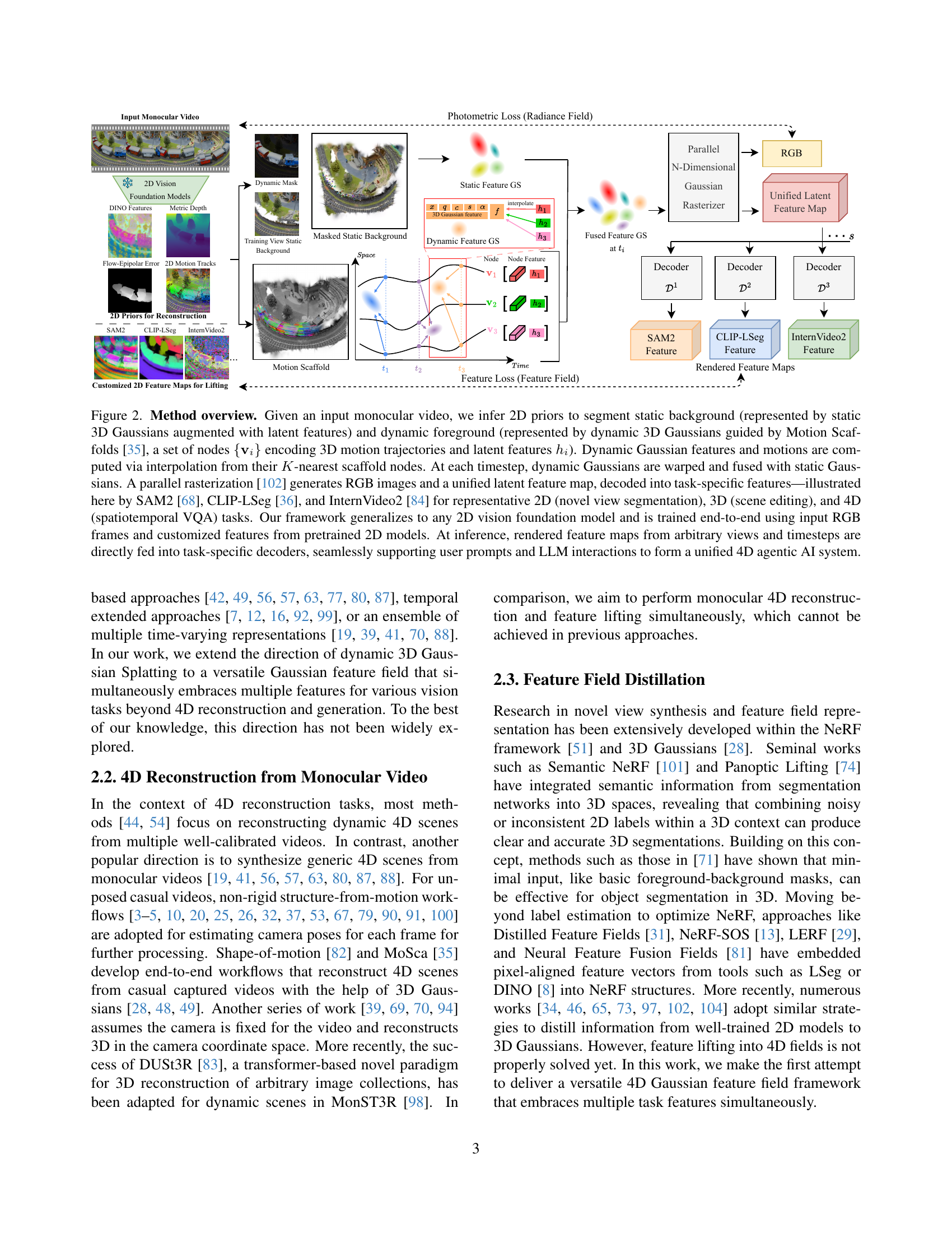
🔼 Figure 2 illustrates the Feature4X framework’s architecture for processing monocular video input into a 4D representation suitable for various AI tasks. 2D priors are used to delineate static and dynamic elements. Static elements are represented by static 3D Gaussians combined with latent features, while dynamic elements are modeled using dynamic 3D Gaussians guided by Motion Scaffolds (a graph structure encoding motion trajectories and latent features). These Gaussians are then combined and processed through a parallel rasterization technique generating RGB images and a unified latent feature map. This map is subsequently decoded into task-specific features, as exemplified using SAM2, CLIP-LSeg, and InternVideo2 for 2D, 3D, and 4D tasks respectively. The framework’s adaptability to various 2D vision models and end-to-end training approach are also highlighted, demonstrating its ability to seamlessly support user prompts and LLM interactions for creating a unified 4D agentic AI system.
read the caption
Figure 2: Method overview. Given an input monocular video, we infer 2D priors to segment static background (represented by static 3D Gaussians augmented with latent features) and dynamic foreground (represented by dynamic 3D Gaussians guided by Motion Scaffolds [35], a set of nodes {𝐯i}subscript𝐯𝑖\{\mathbf{v}_{i}\}{ bold_v start_POSTSUBSCRIPT italic_i end_POSTSUBSCRIPT } encoding 3D motion trajectories and latent features hisubscriptℎ𝑖h_{i}italic_h start_POSTSUBSCRIPT italic_i end_POSTSUBSCRIPT). Dynamic Gaussian features and motions are computed via interpolation from their K𝐾Kitalic_K-nearest scaffold nodes. At each timestep, dynamic Gaussians are warped and fused with static Gaussians. A parallel rasterization [102] generates RGB images and a unified latent feature map, decoded into task-specific features—illustrated here by SAM2 [68], CLIP-LSeg [36], and InternVideo2 [84] for representative 2D (novel view segmentation), 3D (scene editing), and 4D (spatiotemporal VQA) tasks. Our framework generalizes to any 2D vision foundation model and is trained end-to-end using input RGB frames and customized features from pretrained 2D models. At inference, rendered feature maps from arbitrary views and timesteps are directly fed into task-specific decoders, seamlessly supporting user prompts and LLM interactions to form a unified 4D agentic AI system.

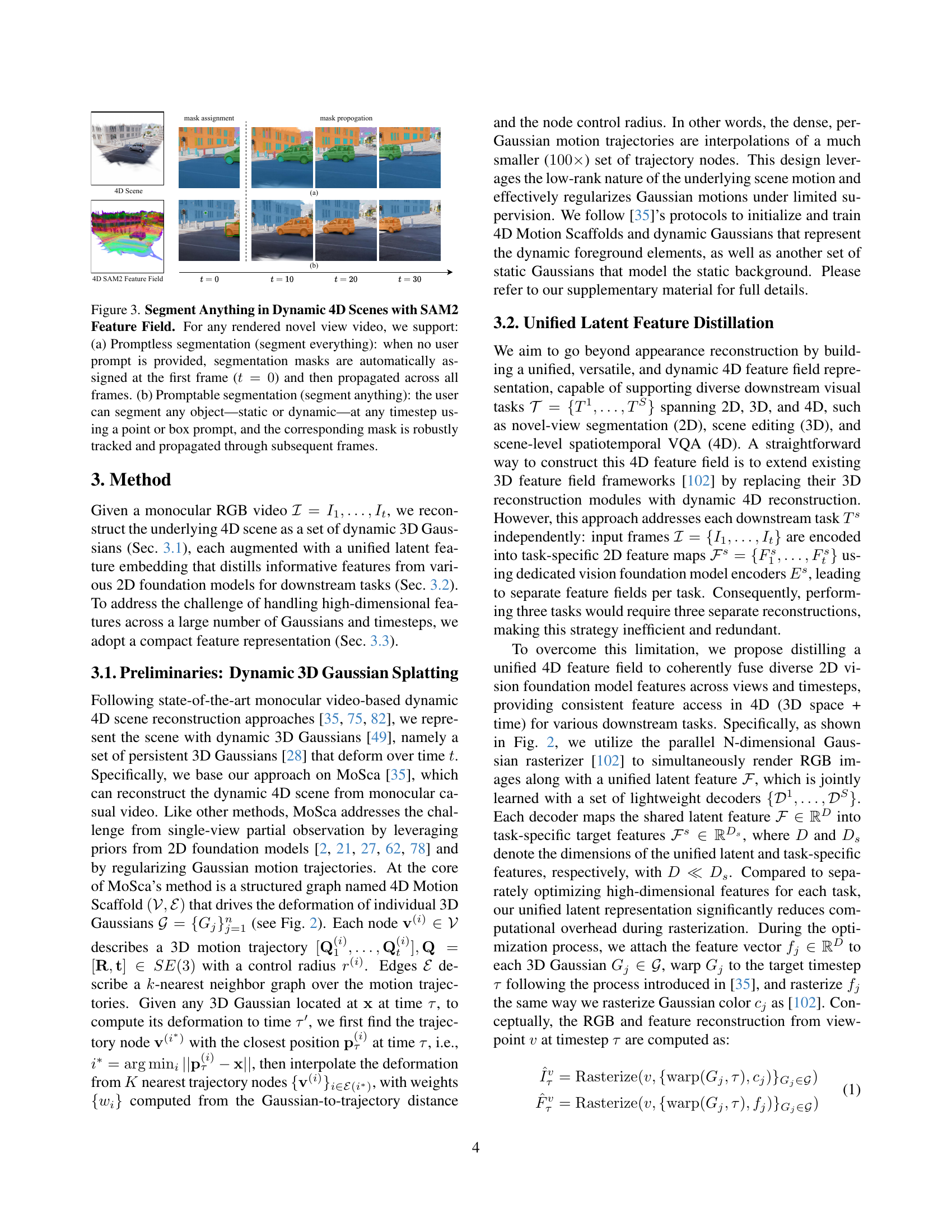
🔼 Figure 3 demonstrates the capabilities of Feature4X in performing semantic segmentation on dynamic 4D scenes using the Segment Anything Model (SAM2). It showcases two modes: (a) Promptless segmentation, where the system automatically segments all objects in the first frame (t=0) and propagates these masks consistently across subsequent frames, handling both static and dynamic content. (b) Promptable segmentation, which allows users to interactively segment any object (static or dynamic) at any point in time simply by providing a point or box prompt. The system then accurately tracks and propagates this mask through the rest of the video. This highlights the versatility and robustness of Feature4X in handling complex 4D scenes.
read the caption
Figure 3: Segment Anything in Dynamic 4D Scenes with SAM2 Feature Field. For any rendered novel view video, we support: (a) Promptless segmentation (segment everything): when no user prompt is provided, segmentation masks are automatically assigned at the first frame (t=0𝑡0t=0italic_t = 0) and then propagated across all frames. (b) Promptable segmentation (segment anything): the user can segment any object—static or dynamic—at any timestep using a point or box prompt, and the corresponding mask is robustly tracked and propagated through subsequent frames.

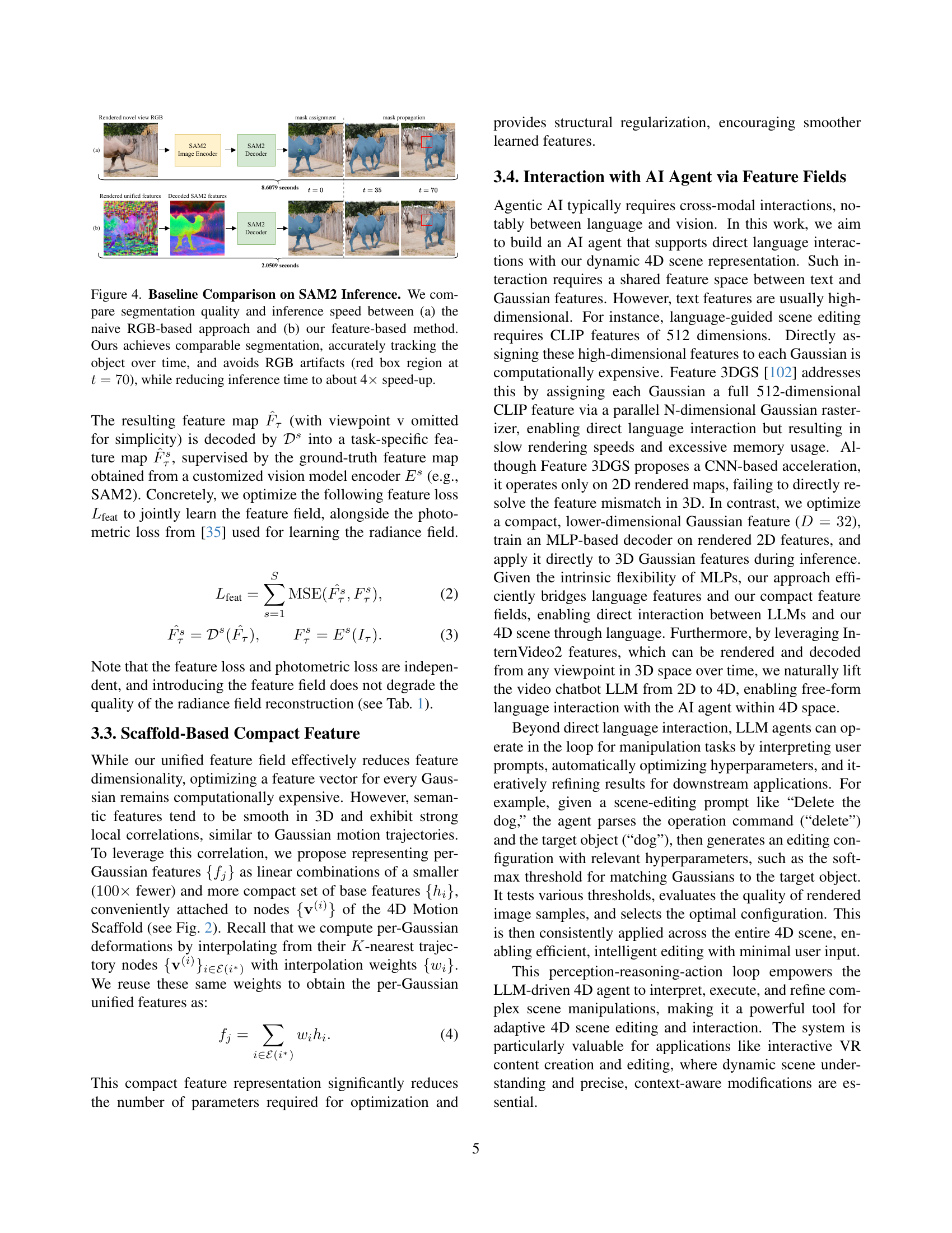
🔼 Figure 4 presents a comparison of two methods for SAM2 inference: a naive RGB-based approach and a novel feature-based approach. The RGB-based approach processes the raw RGB video frames directly through the SAM2 model, while the feature-based approach utilizes a learned compact 4D feature field representation to achieve segmentation. The results demonstrate that the feature-based method achieves comparable segmentation accuracy, accurately tracking the object across frames. Importantly, it avoids the RGB artifacts observed in the naive RGB-based approach, specifically around time step 70. The feature-based method also offers a significant speed-up in inference time, achieving approximately four times faster processing than the RGB-based approach.
read the caption
Figure 4: Baseline Comparison on SAM2 Inference. We compare segmentation quality and inference speed between (a) the naive RGB-based approach and (b) our feature-based method. Ours achieves comparable segmentation, accurately tracking the object over time, and avoids RGB artifacts (red box region at t=70𝑡70t=70italic_t = 70), while reducing inference time to about 4×\times× speed-up.

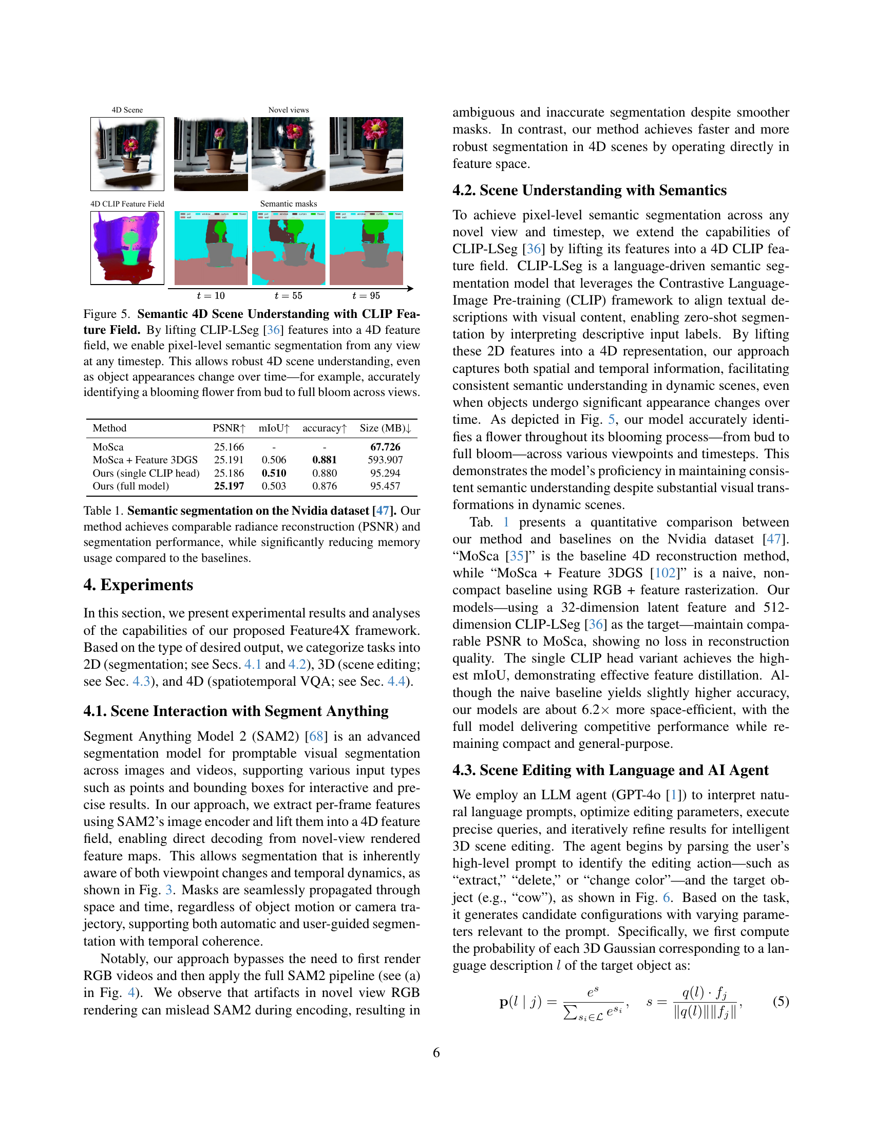
🔼 Figure 5 demonstrates the capability of Feature4X to perform semantic 4D scene understanding. By incorporating CLIP-LSeg features into a 4D feature field, the model achieves pixel-level semantic segmentation from any viewpoint at any point in time. This addresses a key challenge in 3D/4D vision: maintaining consistent semantic understanding even as object appearance changes dynamically throughout the video. The example of a blooming flower, accurately identified from bud to full bloom across multiple views, showcases this robust 4D scene understanding capability.
read the caption
Figure 5: Semantic 4D Scene Understanding with CLIP Feature Field. By lifting CLIP-LSeg [36] features into a 4D feature field, we enable pixel-level semantic segmentation from any view at any timestep. This allows robust 4D scene understanding, even as object appearances change over time—for example, accurately identifying a blooming flower from bud to full bloom across views.

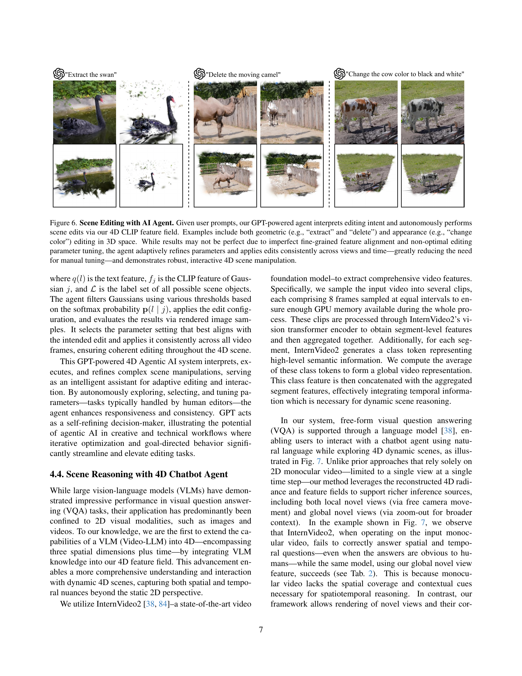
🔼 This figure showcases the capabilities of the LLM-powered AI agent in editing 4D scenes. The agent takes high-level natural language instructions (e.g., ‘Extract the swan’, ‘Delete the moving camel’, ‘Change the cow color to black and white’) and uses the 4D CLIP feature field to perform the edits. The edits can involve geometric changes (like extracting or deleting objects) or changes in appearance (like altering an object’s color). While the results might not be perfect due to limitations in aligning fine-grained features or finding optimal editing parameters, the AI agent iteratively refines these parameters and ensures consistent application of edits across different viewpoints and time steps. This significantly simplifies the editing process and enables robust, interactive 4D scene manipulation.
read the caption
Figure 6: Scene Editing with AI Agent. Given user prompts, our GPT-powered agent interprets editing intent and autonomously performs scene edits via our 4D CLIP feature field. Examples include both geometric (e.g., “extract” and “delete”) and appearance (e.g., “change color”) editing in 3D space. While results may not be perfect due to imperfect fine-grained feature alignment and non-optimal editing parameter tuning, the agent adaptively refines parameters and applies edits consistently across views and time—greatly reducing the need for manual tuning—and demonstrates robust, interactive 4D scene manipulation.
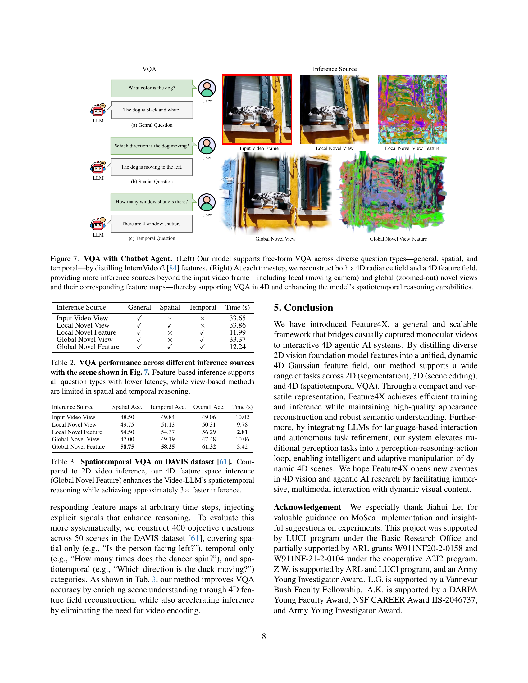
🔼 Figure 7 illustrates the model’s ability to answer visual questions (VQA) using a chatbot interface. The left side shows the diverse question types supported: general, spatial, and temporal questions. The core of this capability comes from leveraging InternVideo2’s features. The right panel highlights the model’s 4D reconstruction, producing both a 4D radiance field and a 4D feature field. This provides access to richer inference sources than just the original input video. These include novel views (both local, from a moving camera, and global, zoomed-out) and their corresponding feature maps. This approach is crucial for robust spatiotemporal reasoning in VQA.
read the caption
Figure 7: VQA with Chatbot Agent. (Left) Our model supports free-form VQA across diverse question types—general, spatial, and temporal—by distilling InternVideo2 [84] features. (Right) At each timestep, we reconstruct both a 4D radiance field and a 4D feature field, providing more inference sources beyond the input video frame—including local (moving camera) and global (zoomed-out) novel views and their corresponding feature maps—thereby supporting VQA in 4D and enhancing the model’s spatiotemporal reasoning capabilities.

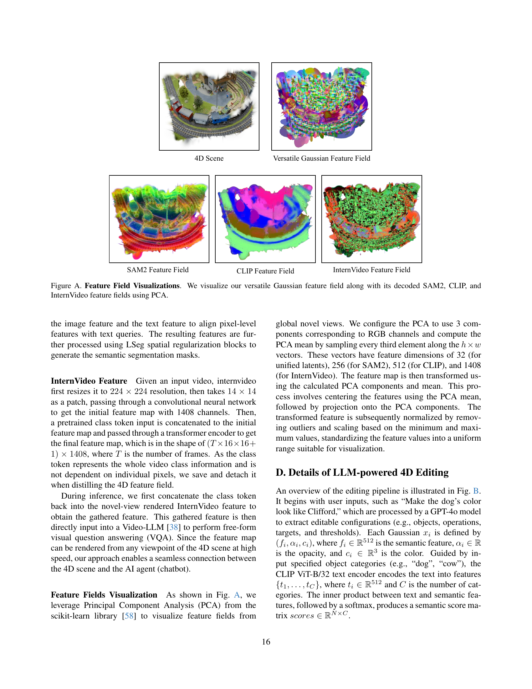
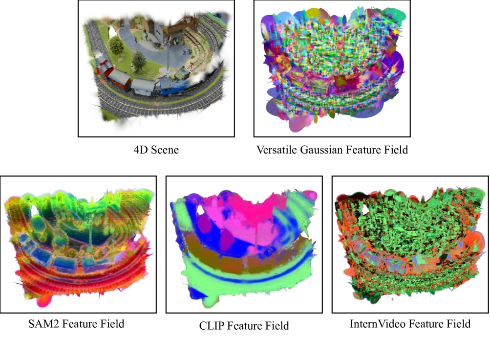
🔼 This figure visualizes the versatile Gaussian feature field developed in the Feature4X framework. It uses Principal Component Analysis (PCA) to reduce the dimensionality of the feature fields for better visualization. The visualization includes the unified latent feature field and its decoded versions for three different 2D foundation models: Segment Anything (SAM2), CLIP-LSeg, and InternVideo. Each model’s decoded feature field provides a different perspective on the underlying 4D scene representation, highlighting the versatility of the Feature4X framework in adapting to various downstream tasks.
read the caption
Figure A: Feature Field Visualizations. We visualize our versatile Gaussian feature field along with its decoded SAM2, CLIP, and InternVideo feature fields using PCA.

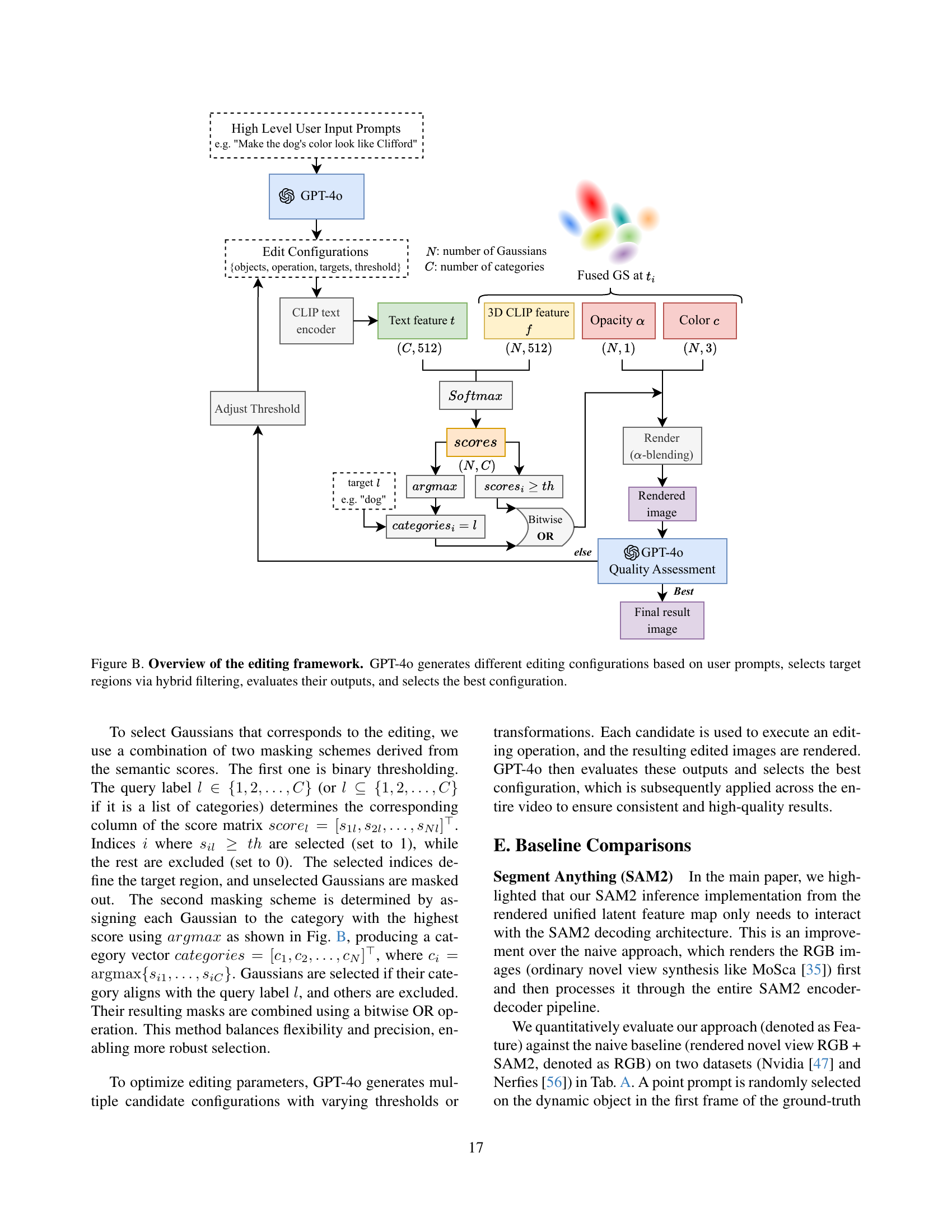
🔼 This figure illustrates the 4D scene editing framework. It begins with a user providing a high-level prompt (e.g., ‘Make the dog’s color look like Clifford’). This prompt is processed by GPT-40, a large language model, to generate different editing configurations. These configurations include details like which objects to edit, what operations to perform, the specific targets for the edits, and threshold settings. The model then uses a hybrid filtering method to identify the relevant Gaussians (points in a 3D Gaussian splatting representation) within the 4D scene that correspond to the targeted objects. The system then applies the selected edit operation and renders the result. Finally, the GPT-40 model evaluates the rendered image quality and selects the best configuration, ensuring consistency and high quality results across the 4D scene.
read the caption
Figure B: Overview of the editing framework. GPT-4o generates different editing configurations based on user prompts, selects target regions via hybrid filtering, evaluates their outputs, and selects the best configuration.

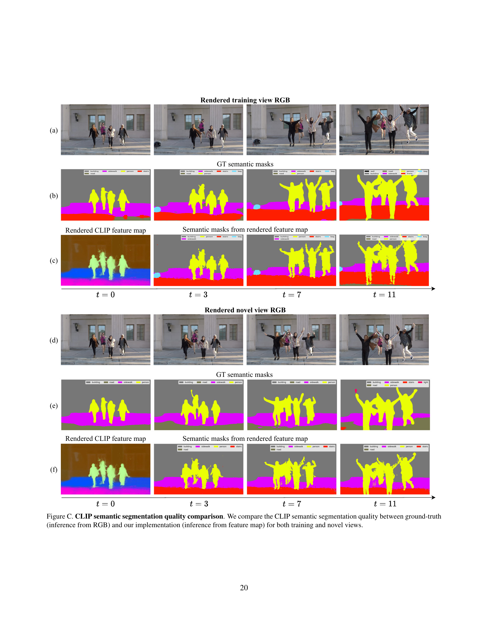
🔼 This figure compares the semantic segmentation results obtained using CLIP features. Two methods are compared: one using ground-truth RGB images and the other using the proposed method’s feature maps. The comparison is done for both training and novel (unseen) views to show how well the proposed method generalizes to new viewpoints. The results visually demonstrate the effectiveness of the proposed method for accurate and consistent semantic segmentation across different views, even without directly using the full RGB image information.
read the caption
Figure C: CLIP semantic segmentation quality comparison. We compare the CLIP semantic segmentation quality between ground-truth (inference from RGB) and our implementation (inference from feature map) for both training and novel views.

🔼 This figure compares the segmentation quality achieved using the Segment Anything Model 2 (SAM2) with different dimensions for the unified latent feature maps. The results show that a 32-dimensional unified latent feature map produces the best performing SAM2 segmentation, accurately tracking the object over time and avoiding artifacts present in the results from other dimensions.
read the caption
Figure D: SAM2 segmentation quality comparison for different dimensions of unified latent feature maps Best performing SAM2 segmentation is derived from the 32-dimensional unified latent feature map.

🔼 This figure shows the training time taken for different dimensions of the unified latent feature map. It demonstrates the trade-off between model complexity and training efficiency. As the dimension of the latent feature increases, so does the training time. This is because higher dimensions increase the number of parameters the model needs to learn, leading to longer training times.
read the caption
Figure E: Training Time vs Unified Latent Feature Dimensions We show the training time required with different dimensions of unified latent feature map.

🔼 This figure demonstrates the relationship between the dimensionality of the unified latent feature map and the time needed for rendering. As the dimensionality increases, the rendering time also increases, highlighting a trade-off between feature representation complexity and computational efficiency. The plot likely shows an exponential or near-exponential increase in rendering time as the dimension increases, indicating that higher-dimensional features significantly increase computational demands during the rendering process.
read the caption
Figure F: Rendering Time vs Unified Latent Feature Dimensions We show the rendering time required for different dimensions of unified latent feature map.

🔼 This figure shows a graph illustrating the relationship between the training time and the dimensionality of rendered CLIP features. Higher dimensional rendered CLIP features lead to longer training times. This demonstrates a trade-off between model complexity and training efficiency.
read the caption
Figure G: Training Time vs CLIP Feature Dimensions We show the training time required with different dimensions of rendered CLIP features.

🔼 Figure H illustrates the relationship between the rendering time and the dimensions of rendered CLIP features. The x-axis represents the different dimensions of the rendered CLIP features used in the experiment, while the y-axis shows the corresponding rendering time. The graph likely demonstrates that increasing the dimensions of the CLIP features significantly increases the rendering time required. This suggests a trade-off between feature richness and computational efficiency.
read the caption
Figure H: Rendering Time vs CLIP Feature Dimensions We show the rendering time required for different dimensions of rendered CLIP features.

🔼 This figure presents the results of an ablation study that examines how different dimensions of rendered CLIP features affect the mean Intersection over Union (mIoU) score in semantic segmentation. The x-axis represents the dimension of the rendered CLIP features, while the y-axis shows the corresponding mIoU score. The graph helps to determine the optimal dimensionality for achieving a balance between performance and computational efficiency.
read the caption
Figure I: mIoU vs CLIP Feature Dimensions We show mIoU with respect to different rendered CLIP feature dimensions.
More on tables
| Inference Source | General | Spatial | Temporal | Time (s) |
|---|---|---|---|---|
| Input Video View | ✓ | 33.65 | ||
| Local Novel View | ✓ | ✓ | 33.86 | |
| Local Novel Feature | ✓ | ✓ | 11.99 | |
| Global Novel View | ✓ | ✓ | 33.37 | |
| Global Novel Feature | ✓ | ✓ | ✓ | 12.24 |
🔼 This table presents the performance of Visual Question Answering (VQA) using different inference sources on the scene depicted in Figure 7. The inference sources are categorized into view-based (input video view, local novel view, global novel view) and feature-based (local novel view feature, global novel view feature). The table shows the accuracy of answering general, spatial, and temporal questions using each inference source. It highlights that feature-based inference achieves higher accuracy and requires less time for all question types compared to view-based methods, indicating that feature-based inference is better suited for spatiotemporal reasoning tasks.
read the caption
Table 2: VQA performance across different inference sources with the scene shown in Fig. 7. Feature-based inference supports all question types with lower latency, while view-based methods are limited in spatial and temporal reasoning.
| Inference Source | Spatial Acc. | Temporal Acc. | Overall Acc. | Time (s) |
|---|---|---|---|---|
| Input Video View | 48.50 | 49.84 | 49.06 | 10.02 |
| Local Novel View | 49.75 | 51.13 | 50.31 | 9.78 |
| Local Novel Feature | 54.50 | 54.37 | 56.29 | 2.81 |
| Global Novel View | 47.00 | 49.19 | 47.48 | 10.06 |
| Global Novel Feature | 58.75 | 58.25 | 61.32 | 3.42 |
🔼 This table presents a quantitative comparison of spatiotemporal Visual Question Answering (VQA) performance on the DAVIS dataset. It compares the accuracy and inference time of different methods for answering various types of questions (general, spatial, and temporal) about a video scene. The methods include using only the input video, local novel views, features from local novel views, global novel views, and features from global novel views. The key finding is that using our 4D feature space (Global Novel Feature) significantly improves the Video-LLM’s ability to reason about both space and time in the video, while also achieving a threefold speedup in inference compared to 2D video inference.
read the caption
Table 3: Spatiotemporal VQA on DAVIS dataset [61]. Compared to 2D video inference, our 4D feature space inference (Global Novel Feature) enhances the Video-LLM’s spatiotemporal reasoning while achieving approximately 3×\times× faster inference.
| NVIDIA | Exp1 | Exp2 | Exp3 | Mean | Time (s) |
|---|---|---|---|---|---|
| RGB | 0.656 | 0.246 | 0.467 | 0.456 | 1.83 |
| Feature | 0.761 | 0.728 | 0.727 | 0.739 | 1.01 |
🔼 This table presents the mean Intersection over Union (mIoU) scores achieved by the Segment Anything Model 2 (SAM2) on the NVIDIA and Nerfies datasets. It compares the performance of two approaches: a baseline method using RGB images directly and the proposed Feature4X method which uses distilled features. The results are presented for three separate experiments (Exp1, Exp2, Exp3) to showcase the robustness and stability of the Feature4X method. Inference time is also reported for each approach.
read the caption
Table A: SAM2 Quantitative Results (mIoU) on NVIDIA and Nerfies Datasets.
| Nerfies | Exp1 | Exp2 | Exp3 | Mean | Time (s) |
|---|---|---|---|---|---|
| RGB | 0.484 | 0.536 | 0.538 | 0.519 | 9.10 |
| Feature | 0.560 | 0.662 | 0.561 | 0.594 | 3.10 |
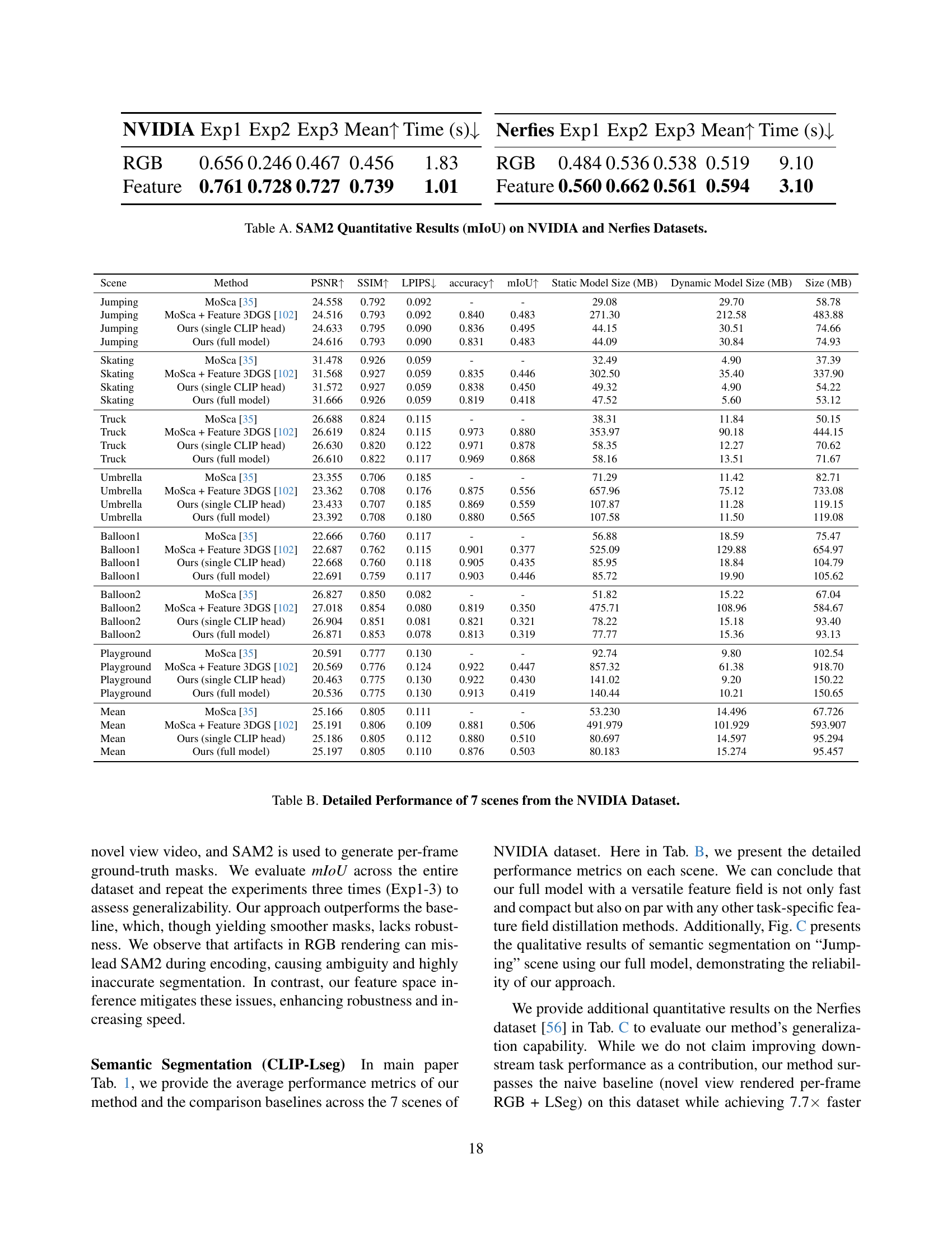
🔼 Table B presents a detailed quantitative analysis of the proposed Feature4X model’s performance on seven distinct scenes from the NVIDIA dataset. For each scene, the table compares the performance metrics of four different methods: the baseline MoSca model, MoSca augmented with Feature 3DGS, Feature4X with a single CLIP head, and the full Feature4X model. The metrics reported include PSNR, SSIM, LPIPS, accuracy, and mIoU, providing a comprehensive evaluation of the model’s ability to reconstruct the scene accurately, and its effectiveness in performing both semantic segmentation and spatiotemporal reasoning. The table also shows the model sizes (static and dynamic) for each method, offering insights into memory usage and computational efficiency.
read the caption
Table B: Detailed Performance of 7 scenes from the NVIDIA Dataset.
| Scene | Method | PSNR | SSIM | LPIPS | accuracy | mIoU | Static Model Size (MB) | Dynamic Model Size (MB) | Size (MB) |
|---|---|---|---|---|---|---|---|---|---|
| Jumping | MoSca [35] | 24.558 | 0.792 | 0.092 | - | - | 29.08 | 29.70 | 58.78 |
| Jumping | MoSca + Feature 3DGS [102] | 24.516 | 0.793 | 0.092 | 0.840 | 0.483 | 271.30 | 212.58 | 483.88 |
| Jumping | Ours (single CLIP head) | 24.633 | 0.795 | 0.090 | 0.836 | 0.495 | 44.15 | 30.51 | 74.66 |
| Jumping | Ours (full model) | 24.616 | 0.793 | 0.090 | 0.831 | 0.483 | 44.09 | 30.84 | 74.93 |
| Skating | MoSca [35] | 31.478 | 0.926 | 0.059 | - | - | 32.49 | 4.90 | 37.39 |
| Skating | MoSca + Feature 3DGS [102] | 31.568 | 0.927 | 0.059 | 0.835 | 0.446 | 302.50 | 35.40 | 337.90 |
| Skating | Ours (single CLIP head) | 31.572 | 0.927 | 0.059 | 0.838 | 0.450 | 49.32 | 4.90 | 54.22 |
| Skating | Ours (full model) | 31.666 | 0.926 | 0.059 | 0.819 | 0.418 | 47.52 | 5.60 | 53.12 |
| Truck | MoSca [35] | 26.688 | 0.824 | 0.115 | - | - | 38.31 | 11.84 | 50.15 |
| Truck | MoSca + Feature 3DGS [102] | 26.619 | 0.824 | 0.115 | 0.973 | 0.880 | 353.97 | 90.18 | 444.15 |
| Truck | Ours (single CLIP head) | 26.630 | 0.820 | 0.122 | 0.971 | 0.878 | 58.35 | 12.27 | 70.62 |
| Truck | Ours (full model) | 26.610 | 0.822 | 0.117 | 0.969 | 0.868 | 58.16 | 13.51 | 71.67 |
| Umbrella | MoSca [35] | 23.355 | 0.706 | 0.185 | - | - | 71.29 | 11.42 | 82.71 |
| Umbrella | MoSca + Feature 3DGS [102] | 23.362 | 0.708 | 0.176 | 0.875 | 0.556 | 657.96 | 75.12 | 733.08 |
| Umbrella | Ours (single CLIP head) | 23.433 | 0.707 | 0.185 | 0.869 | 0.559 | 107.87 | 11.28 | 119.15 |
| Umbrella | Ours (full model) | 23.392 | 0.708 | 0.180 | 0.880 | 0.565 | 107.58 | 11.50 | 119.08 |
| Balloon1 | MoSca [35] | 22.666 | 0.760 | 0.117 | - | - | 56.88 | 18.59 | 75.47 |
| Balloon1 | MoSca + Feature 3DGS [102] | 22.687 | 0.762 | 0.115 | 0.901 | 0.377 | 525.09 | 129.88 | 654.97 |
| Balloon1 | Ours (single CLIP head) | 22.668 | 0.760 | 0.118 | 0.905 | 0.435 | 85.95 | 18.84 | 104.79 |
| Balloon1 | Ours (full model) | 22.691 | 0.759 | 0.117 | 0.903 | 0.446 | 85.72 | 19.90 | 105.62 |
| Balloon2 | MoSca [35] | 26.827 | 0.850 | 0.082 | - | - | 51.82 | 15.22 | 67.04 |
| Balloon2 | MoSca + Feature 3DGS [102] | 27.018 | 0.854 | 0.080 | 0.819 | 0.350 | 475.71 | 108.96 | 584.67 |
| Balloon2 | Ours (single CLIP head) | 26.904 | 0.851 | 0.081 | 0.821 | 0.321 | 78.22 | 15.18 | 93.40 |
| Balloon2 | Ours (full model) | 26.871 | 0.853 | 0.078 | 0.813 | 0.319 | 77.77 | 15.36 | 93.13 |
| Playground | MoSca [35] | 20.591 | 0.777 | 0.130 | - | - | 92.74 | 9.80 | 102.54 |
| Playground | MoSca + Feature 3DGS [102] | 20.569 | 0.776 | 0.124 | 0.922 | 0.447 | 857.32 | 61.38 | 918.70 |
| Playground | Ours (single CLIP head) | 20.463 | 0.775 | 0.130 | 0.922 | 0.430 | 141.02 | 9.20 | 150.22 |
| Playground | Ours (full model) | 20.536 | 0.775 | 0.130 | 0.913 | 0.419 | 140.44 | 10.21 | 150.65 |
| Mean | MoSca [35] | 25.166 | 0.805 | 0.111 | - | - | 53.230 | 14.496 | 67.726 |
| Mean | MoSca + Feature 3DGS [102] | 25.191 | 0.806 | 0.109 | 0.881 | 0.506 | 491.979 | 101.929 | 593.907 |
| Mean | Ours (single CLIP head) | 25.186 | 0.805 | 0.112 | 0.880 | 0.510 | 80.697 | 14.597 | 95.294 |
| Mean | Ours (full model) | 25.197 | 0.805 | 0.110 | 0.876 | 0.503 | 80.183 | 15.274 | 95.457 |
🔼 This table presents a quantitative comparison of semantic segmentation performance on the Nerfies dataset. It compares the mean Intersection over Union (mIoU), accuracy, and inference time for different methods, including RGB-based and feature-based approaches, across several scenes (Broom, Curls, Tails, Toby-sit). The results showcase the improved efficiency and comparable segmentation accuracy achieved by the feature-based method compared to the RGB-based method.
read the caption
Table C: Semantic Segmentation Quantitative Results on Nerfies Dataset.
| Nerfies Scene | mIoU | Accuracy | Time (s) | |||
|---|---|---|---|---|---|---|
| RGB | Feature | RGB | Feature | RGB | Feature | |
| Broom | 0.193 | 0.333 | 0.321 | 0.610 | 207.59 | 30.22 |
| Curls | 0.514 | 0.443 | 0.877 | 0.872 | 155.25 | 20.82 |
| Tail | 0.261 | 0.338 | 0.652 | 0.860 | 389.89 | 46.43 |
| Toby-sit | 0.504 | 0.470 | 0.757 | 0.737 | 355.82 | 45.96 |
| Mean | 0.368 | 0.396 | 0.652 | 0.770 | 277.14 | 35.86 |
🔼 This table presents a comprehensive analysis of semantic segmentation performance on the NVIDIA Jumping Scene dataset, using different dimensions for the unified latent feature field. It evaluates the impact of varying the feature dimension on training time (in hours), rendering time (in seconds), mean Intersection over Union (mIoU), and accuracy. Higher dimensions offer potentially more detailed representations, but this comes at a cost of increased computational expense.
read the caption
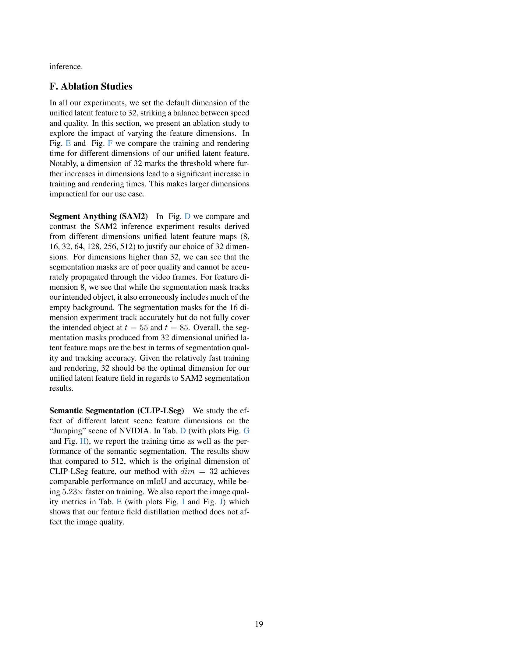
Table D: Evaluation of Semantic Segmentation Performance On NVIDIA Jumping Scene Across Different Dimensions. This table presents the Time, mIoU, and Accuracy corresponding to each dimension level.
| Dimension | 8 | 16 | 32 | 64 | 128 | 256 | 512 |
|---|---|---|---|---|---|---|---|
| Training Time (h) | 2.30 | 2.48 | 2.83 | 3.45 | 4.22 | 8.75 | 14.80 |
| Rendering Time (s) | 4.818 | 4.898 | 4.872 | 4.967 | 5.815 | 10.167 | 16.313 |
| mIoU | 0.468 | 0.483 | 0.482 | 0.485 | 0.471 | 0.494 | 0.497 |
| Accuracy | 0.827 | 0.831 | 0.830 | 0.834 | 0.832 | 0.837 | 0.841 |
🔼 This table presents a quantitative analysis of image quality across various dimensions of the unified latent feature field used in the Feature4X model. Specifically, it shows how Peak Signal-to-Noise Ratio (PSNR), Structural Similarity Index (SSIM), and Learned Perceptual Image Patch Similarity (LPIPS) metrics change as the dimensionality of the feature field is altered. This helps assess the impact of feature dimensionality on the visual fidelity of the reconstructed scenes, specifically for the ‘Jumping’ scene from the NVIDIA dataset.
read the caption
Table E: Evaluation of Image Quality Metrics On NVIDIA Jumping Scene Across Different Dimensions. This table presents the PSNR, SSIM, and LPIPS values corresponding to each dimension level.
Full paper#
