TL;DR#
Diffusion models excel at generation but are slow due to suboptimal step discretization. Existing methods focus on denoising directions. This paper addresses the principled design of stepsize schedules. The authors propose a dynamic programming framework to derive optimal schedules by distilling knowledge from reference trajectories. This tackles computational intensity.
The paper introduces Optimal Stepsize Distillation, reformulating stepsize optimization as recursive error minimization. This method guarantees discretization bounds through optimal substructure exploitation. The distilled schedules show robustness across architectures, ODE solvers, and noise schedules. Experiments demonstrated significant acceleration in text-to-image generation with minimal performance impact.
Key Takeaways#
Why does it matter?#
This paper is important because it addresses the critical issue of computational efficiency in diffusion models, a key barrier to their wider adoption. By providing a theoretically grounded approach to stepsize optimization, it opens new avenues for developing faster and more practical generative models. The framework’s robustness and adaptability also make it a valuable tool for researchers working with various diffusion architectures and applications.
Visual Insights#

🔼 This figure demonstrates the impact of different stepsize schedules on the quality of samples generated by a diffusion model. The leftmost image shows the result of using a standard sampling schedule with 100 steps, producing a high-quality image. The middle image shows the result of using the proposed optimal stepsize schedule, achieving similar quality but using only 10 steps, demonstrating significantly improved efficiency. The rightmost image illustrates the effect of naively reducing the number of steps to 10 without optimizing the schedule, which results in a significantly lower quality image. This illustrates the effectiveness of the proposed optimal stepsize schedule in maintaining sample quality while significantly reducing computation cost.
read the caption
Figure 1: Flux sampling results using different stepsize schedules. Left: Original sampling result using 100100100100 steps. Middle: Optimal stepsize sampling result within 10101010 steps. Right: Naively reducing sampling steps to 10101010.
| Criterion | AYS [25] | GITS [3] | DM [36] | LD3 [32] | OSS |
|---|---|---|---|---|---|
| Training-free | ✓ | ✓ | ✓ | ✕ | ✓ |
| Stability | ✕ | ✓ | ✓ | ✓ | ✓ |
| Solver-aware | ✓ | ✕ | ✕ | ✓ | ✓ |
| Global error | ✕ | ✕ | ✕ | ✓ | ✓ |
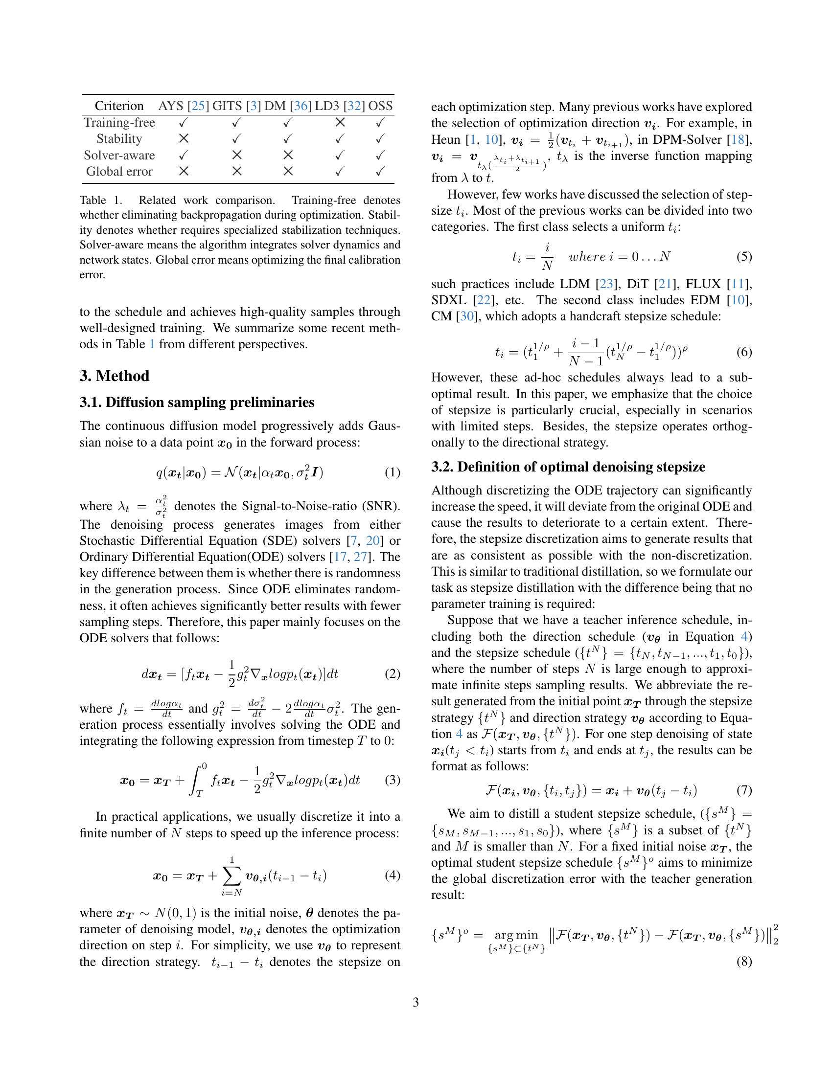
🔼 This table compares different methods for diffusion sampling stepsize optimization. It highlights key characteristics of each method, including whether they require training (backpropagation), need specialized stabilization, consider solver dynamics, and whether they directly aim to minimize the overall error.
read the caption
Table 1: Related work comparison. Training-free denotes whether eliminating backpropagation during optimization. Stability denotes whether requires specialized stabilization techniques. Solver-aware means the algorithm integrates solver dynamics and network states. Global error means optimizing the final calibration error.
In-depth insights#
Optimal Step-Size#
Optimal step-size selection is a critical, yet often underexplored, aspect of diffusion model sampling. While most research focuses on improving the denoising direction, the step-size significantly impacts sampling efficiency and accuracy. A well-designed step-size schedule can dramatically reduce the number of iterations needed for high-quality sample generation. Approaches to optimal step-size selection involve dynamic programming to distill knowledge from reference trajectories, recursive error minimization, and heuristics. Robustness across architectures, ODE solvers, and noise schedules is crucial. Successful methods achieve significant acceleration (e.g., 10x) while maintaining performance, suggesting a significant practical potential for deploying latency-efficient diffusion models. Optimal stepsize operates orthogonally to the directional strategy.
Recursive Subtasks#
The approach smartly decomposes the complex diffusion sampling task into smaller, self-similar subtasks. This recursive structure suggests that finding the optimal solution for a larger step size schedule inherently involves finding optimal solutions for smaller schedules within it. This is a powerful insight as it allows leveraging dynamic programming. The core idea being to leverage known optimal solutions to progressively build better solutions for more complex, larger-scale problems. By breaking the problem down, it can guarantee global discretization bounds through optimal substructure exploitation.
Robustness Analysis#
The robustness analysis comprehensively evaluates the proposed method’s performance across diverse conditions. Noise schedule invariance is assessed using ImageNet-64, demonstrating consistent improvements over baselines regardless of the specific noise schedule employed (EDM, DDIM, Flow Matching). Analyzing performance with varying teacher steps using ImageNet reveals that the method remains effective even with fewer teacher steps (down to 200), indicating a stable search space for dynamic programming. Furthermore, the method showcases robustness across different ODE solver orders with the DiT-XL/2 model on ImageNet 256x256. Crucially, it validates that optimal step scheduling and solver orders work synergistically. Framework generalization is investigated through masked autoregressive generation (MAR) and video diffusion, achieving 100x speedups in MAR while maintaining competitive performance, and preserving visual fidelity in Open-Sora with 10x acceleration, underscoring the method’s broad applicability.
MAR Generation#
In the context of generative modeling, especially within the domain of image synthesis, MAR (likely referring to Masked Autoregressive) generation represents a significant approach. It leverages the autoregressive principle, where the prediction of each element (e.g., pixel) depends on the previously generated elements, forming a chain-like dependency. One of the core strengths of MAR generation lies in its ability to capture complex dependencies within data, leading to high-quality and coherent outputs. The MAR approach is computationally intensive due to its sequential nature, improvements focus on enhancing efficiency while preserving the quality. MAR offers a robust framework for generative tasks, and its continued exploration promises further advancements in the field of image and video synthesis. It plays a crucial role in improving generation performance.
Step Calibration#
Based on the name, step calibration likely addresses the critical issue of adjusting the magnitude of each step taken during the iterative denoising process in diffusion models. It likely involves analyzing and modifying the step sizes to ensure efficient and accurate convergence toward the final generated sample. Step calibration is particularly crucial in few-step sampling scenarios, where suboptimal step sizes can lead to significant deviations from the desired trajectory and compromise output quality. The method might involve strategies such as dynamically adjusting step sizes based on local gradient information or employing a learned calibration function to map noise levels to appropriate step sizes. It aims to achieve a better balance between sampling speed and approximation fidelity by optimizing the step discretization process.
More visual insights#
More on figures

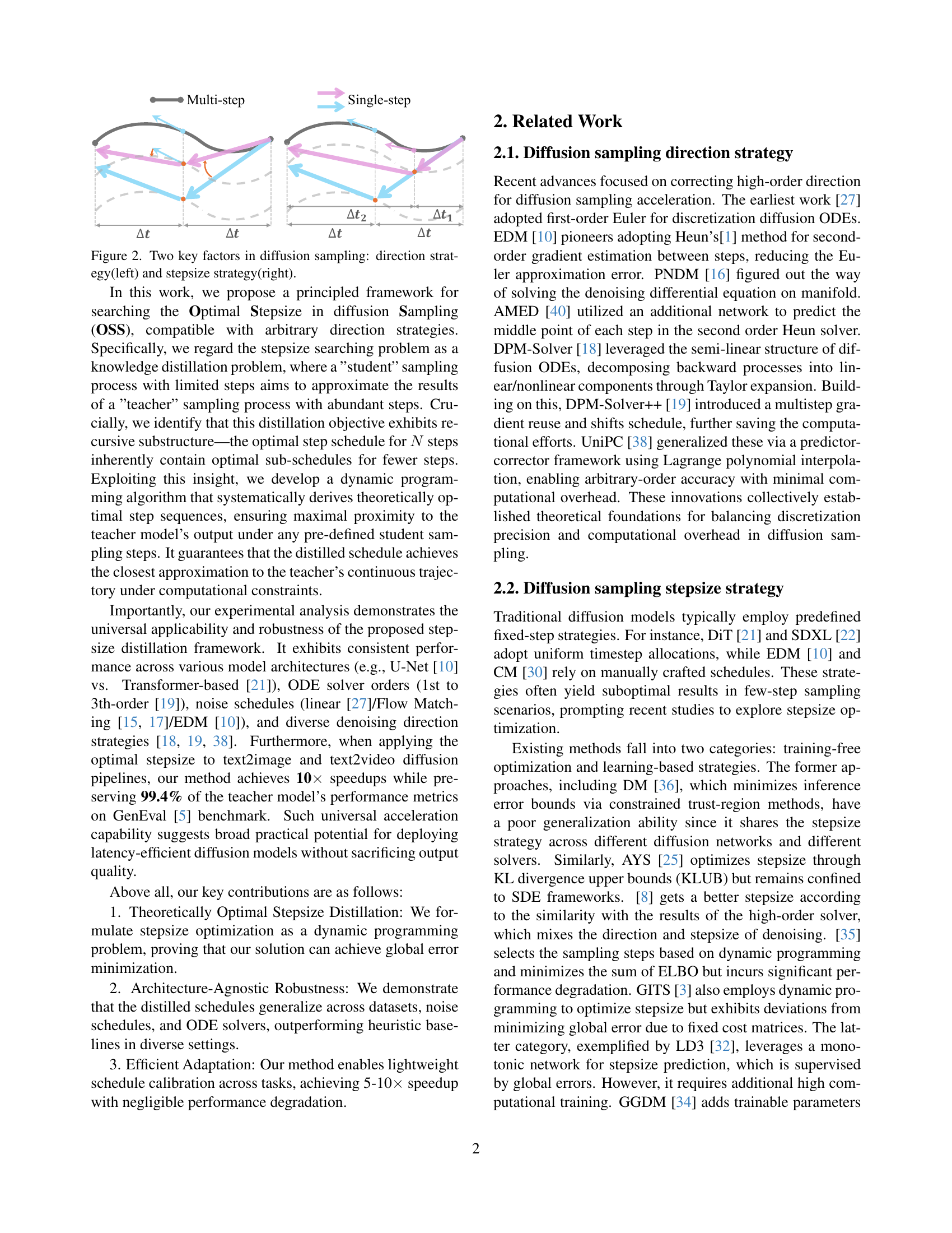
🔼 Figure 2 illustrates the two main factors that influence the outcome of the diffusion sampling process. The left panel demonstrates how different direction strategies (e.g., using different ODE solvers or score functions) affect the trajectory through the probability distribution space. The right panel shows how various stepsize strategies—the size of the steps taken during sampling—influence the trajectory towards the target distribution. The figure highlights that optimizing both the direction and stepsize is critical to efficient and high-quality diffusion sampling.
read the caption
Figure 2: Two key factors in diffusion sampling: direction strategy(left) and stepsize strategy(right).

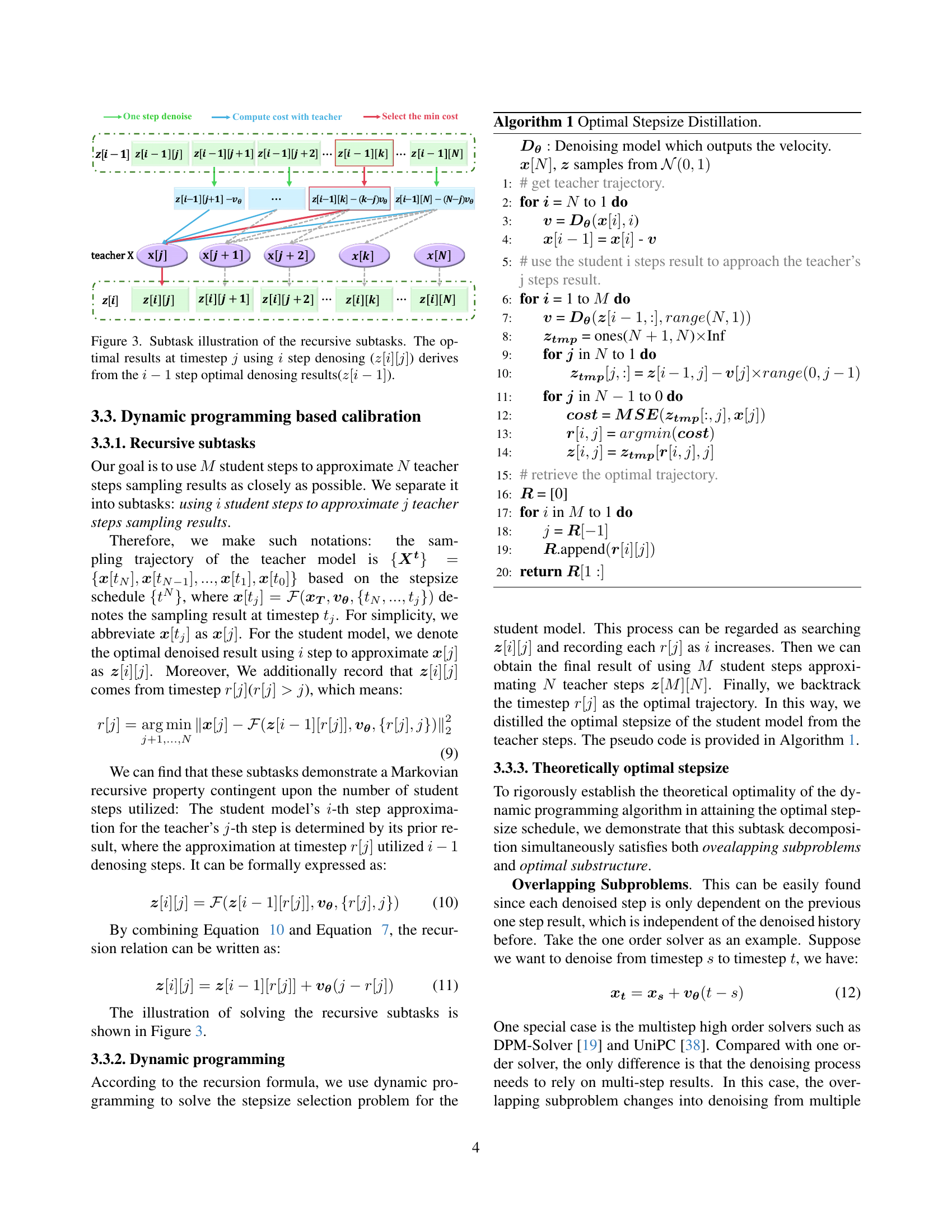
🔼 Figure 3 illustrates the dynamic programming approach used in the Optimal Stepsize Distillation method. It shows how the optimal denoising result at a given timestep (j) and a given number of steps (i) is calculated recursively by utilizing the optimal results from the previous step (i-1). The figure highlights the substructure of the optimization problem, showing how the solution for a larger problem is built upon the solutions of smaller subproblems. This recursive relationship is crucial for the efficiency of the dynamic programming algorithm.
read the caption
Figure 3: Subtask illustration of the recursive subtasks. The optimal results at timestep j𝑗jitalic_j using i𝑖iitalic_i step denosing (z[i][j]𝑧delimited-[]𝑖delimited-[]𝑗z[i][j]italic_z [ italic_i ] [ italic_j ]) derives from the i−1𝑖1i-1italic_i - 1 step optimal denosing results(z[i−1]𝑧delimited-[]𝑖1z[i-1]italic_z [ italic_i - 1 ]).

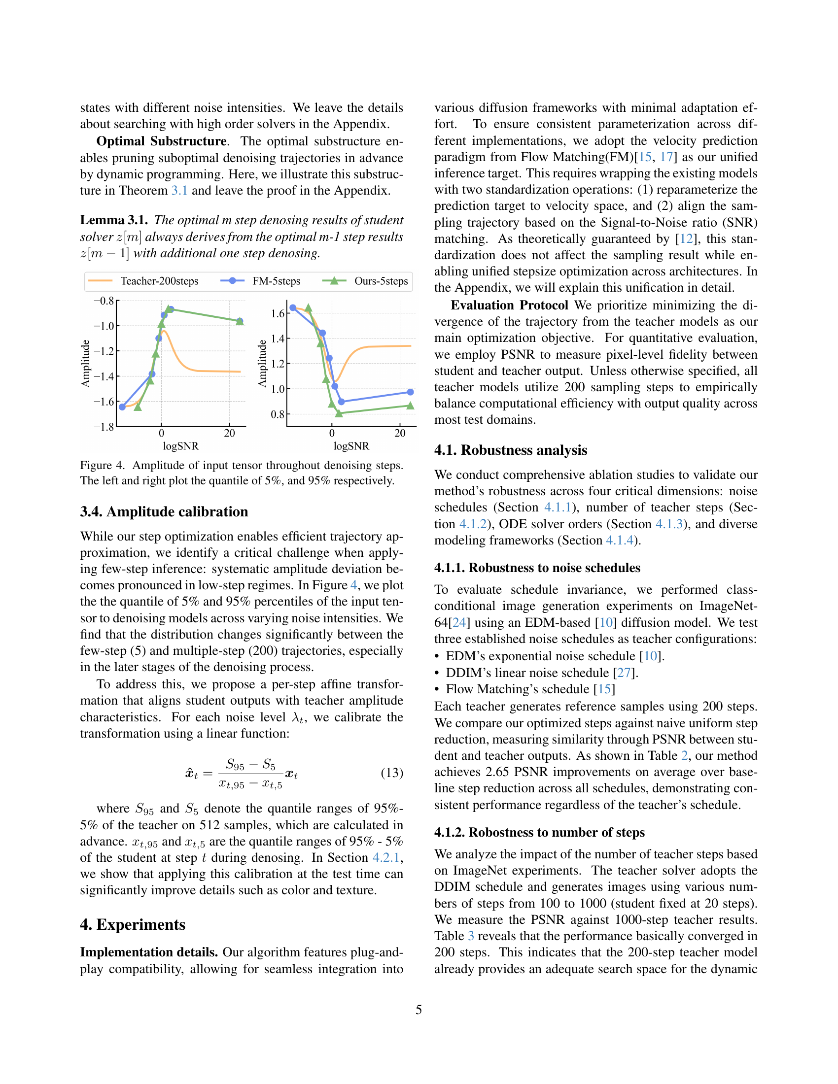
🔼 Figure 4 illustrates the change in the range of the input tensor values during the denoising process. Specifically, the figure displays the 5th and 95th percentiles of the input tensor across all denoising steps. This visualization helps in understanding the dynamic range of data throughout the sampling process and highlights potential amplitude deviations that can occur, especially with a smaller number of steps. The left plot shows the 5th percentile, while the right plot shows the 95th percentile, revealing how the range of tensor values shifts across different steps of the denoising procedure. This is especially relevant for the later steps of the denoising process where the distribution changes significantly between different numbers of steps.
read the caption
Figure 4: Amplitude of input tensor throughout denoising steps. The left and right plot the quantile of 5%, and 95% respectively.

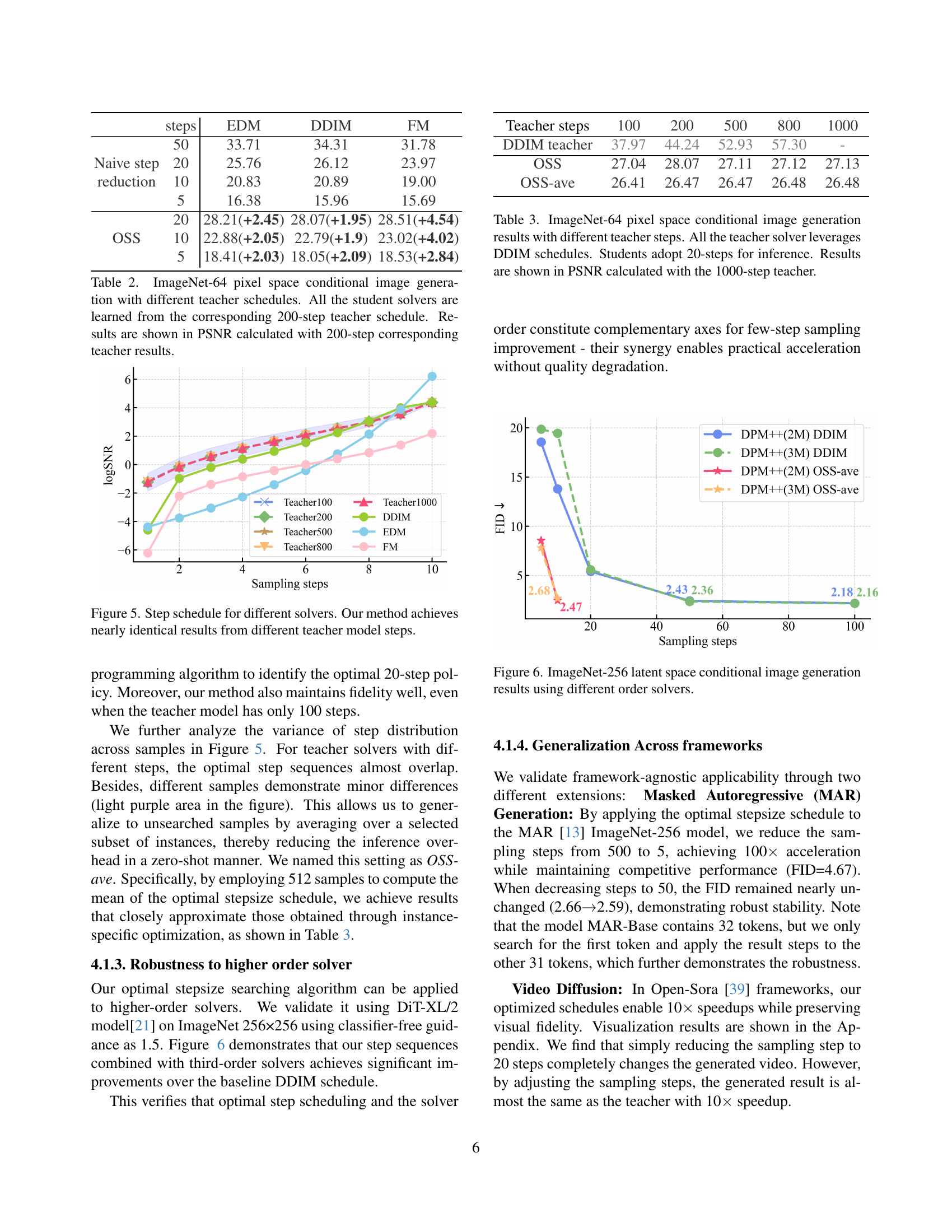
🔼 Figure 5 illustrates the robustness of the proposed optimal stepsize distillation method across different teacher models and ODE solvers. The figure showcases step schedules generated by the method when using teacher models with varying numbers of steps (100, 200, 500, 800, and 1000). The near overlap of the generated step schedules demonstrates that the method is effective at identifying consistent and high-performing stepsize strategies regardless of the teacher model’s training parameters or solver type. The consistent performance across various teacher models highlights the algorithm’s generality and robustness.
read the caption
Figure 5: Step schedule for different solvers. Our method achieves nearly identical results from different teacher model steps.

🔼 This figure displays the results of conditional image generation experiments conducted on the ImageNet-256 dataset using different order solvers. The FID (Fréchet Inception Distance) scores are compared across various diffusion models with different solver orders (e.g. DPM-Solver++ with 2nd and 3rd-order solvers) and different sampling strategies (DDIM and the proposed Optimal Stepsize method). The results demonstrate the impact of higher-order solvers and the proposed optimal stepsize strategy on the quality of generated images and highlight the performance improvements gained through the use of the new method.
read the caption
Figure 6: ImageNet-256 latent space conditional image generation results using different order solvers.

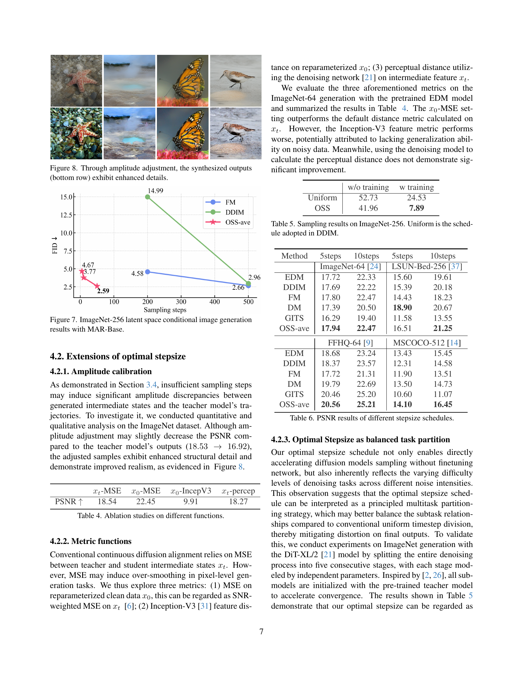
🔼 Figure 7 displays the results of conditional image generation on ImageNet-256 using the MAR-Base model. It illustrates the FID (Fréchet Inception Distance) scores for different sampling methods and numbers of steps, showcasing the impact of the proposed method on reducing the FID score.
read the caption
Figure 7: ImageNet-256 latent space conditional image generation results with MAR-Base.

🔼 Figure 8 presents a comparison of image generation results with and without amplitude calibration. The top row displays images generated using a standard method, showing some blurring and lack of detail. The bottom row shows images generated after applying amplitude calibration. The calibrated images exhibit significantly enhanced details and sharper features, demonstrating the effectiveness of the proposed technique in improving image quality.
read the caption
Figure 8: Through amplitude adjustment, the synthesized outputs (bottom row) exhibit enhanced details.

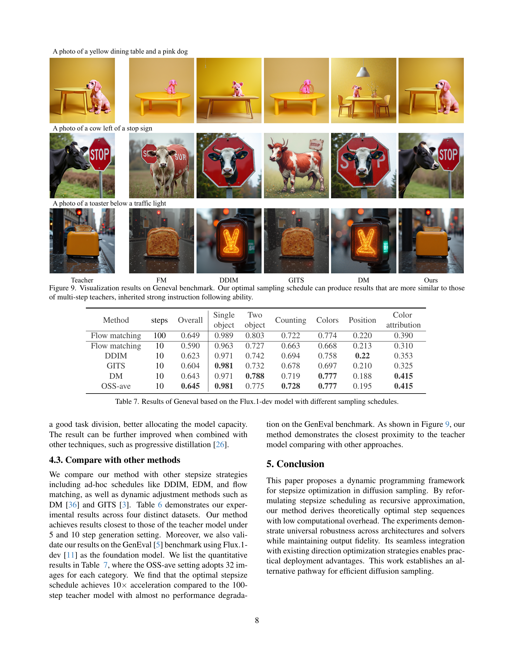
🔼 Figure 9 presents a comparison of image generation results on the Geneval benchmark, a dataset designed to evaluate instruction-following capabilities in image generation models. The figure showcases several models’ outputs, including those using the proposed optimal sampling schedule, and contrasts them with results from models using traditional sampling methods. The comparison highlights the proposed method’s ability to generate images that closely match the quality and instruction-following precision of models trained with significantly more computational steps. This demonstrates the effectiveness of the proposed optimal sampling strategy in reducing computational cost while maintaining high-quality outputs.
read the caption
Figure 9: Visualization results on Geneval benchmark. Our optimal sampling schedule can produce results that are more similar to those of multi-step teachers, inherited strong instruction following ability.

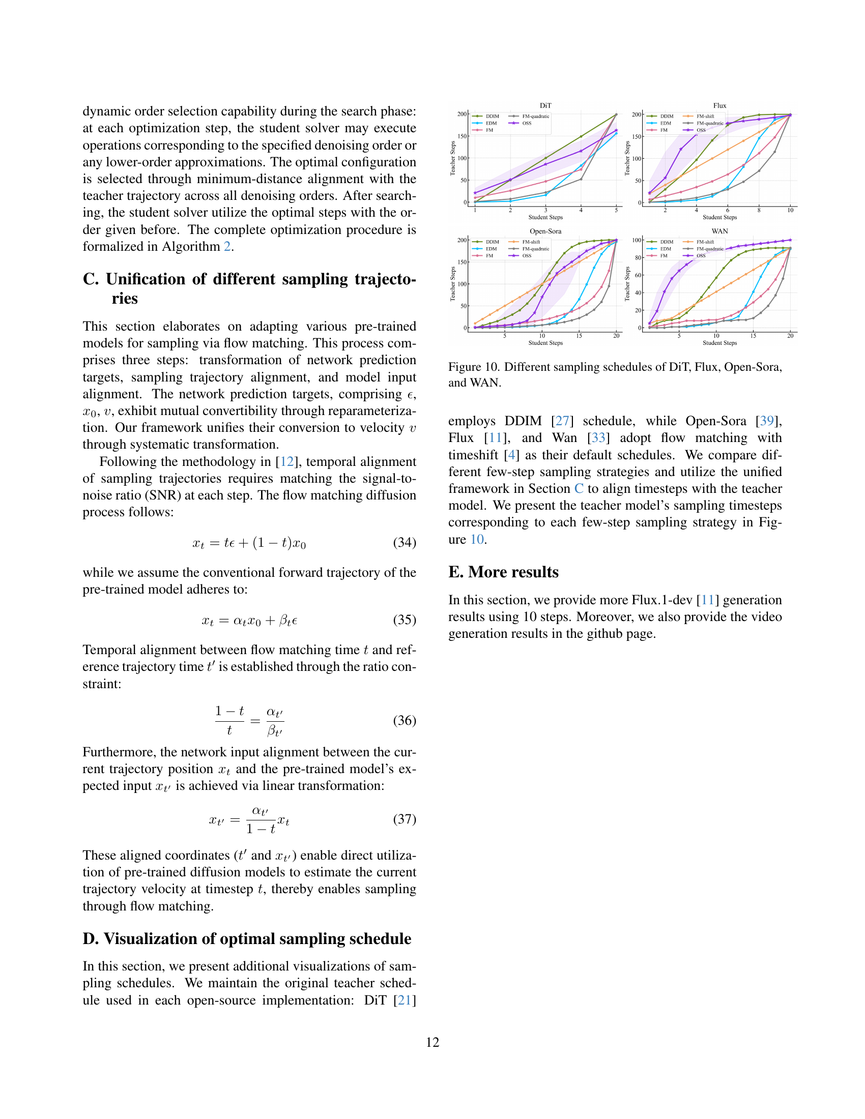
🔼 Figure 10 compares the sampling stepsize schedules used in four different diffusion models: DiT, Flux, Open-Sora, and WAN. Each model uses a different approach to determine the number of steps and their distribution in the sampling process. The figure visually shows how these scheduling strategies differ across the models and highlights their distinct characteristics. This allows for a visual comparison of the different approaches and helps illustrate the range of methodologies employed for efficient sampling in diffusion models.
read the caption
Figure 10: Different sampling schedules of DiT, Flux, Open-Sora, and WAN.

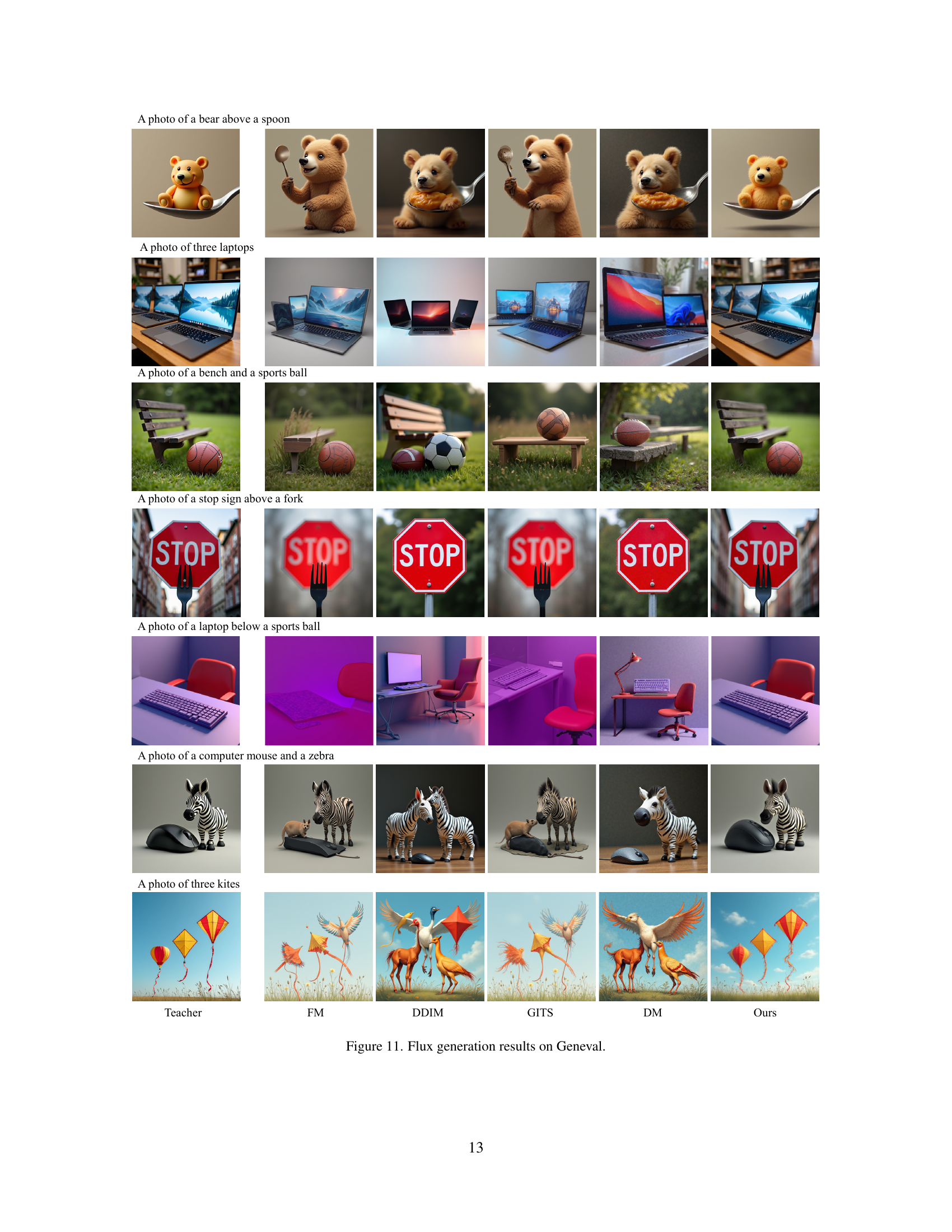
🔼 This figure shows a comparison of image generation results on the Geneval benchmark across different diffusion sampling methods. Each row represents a different prompt from the Geneval dataset. The first column shows the ground truth image. Subsequent columns display images generated using Flow Matching (FM), DDIM, GITS, DM, and the proposed Optimal Stepsize (OSS) method, each with 10 sampling steps. This figure demonstrates that the proposed OSS method produces more realistic and accurate images compared to other methods, especially when using fewer sampling steps.
read the caption
Figure 11: Flux generation results on Geneval.

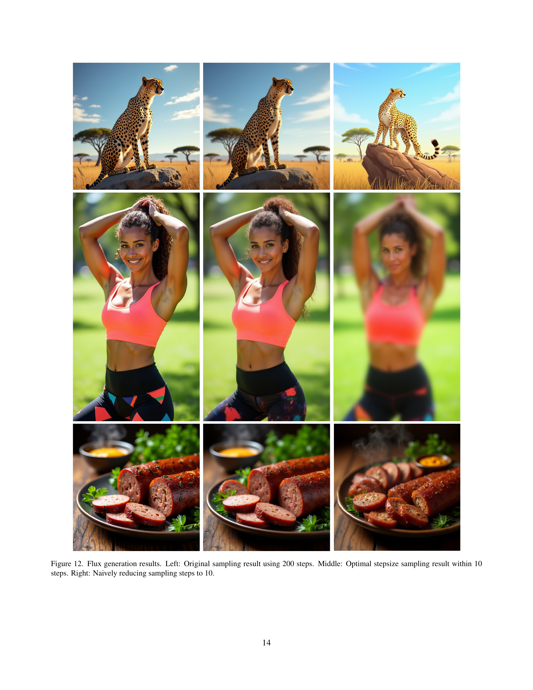
🔼 This figure shows a comparison of image generation results using three different sampling methods. The leftmost image is generated using the original method with 200 sampling steps, showing high-quality details. The middle image uses the proposed optimal stepsize method with only 10 steps, demonstrating that it achieves comparable quality with significantly fewer steps. The rightmost image uses a naive downsampling approach with 10 steps, resulting in a significant loss of detail and image quality. This visually demonstrates the effectiveness of the proposed optimal stepsize method in accelerating the sampling process without sacrificing visual fidelity.
read the caption
Figure 12: Flux generation results. Left: Original sampling result using 200 steps. Middle: Optimal stepsize sampling result within 10 steps. Right: Naively reducing sampling steps to 10.

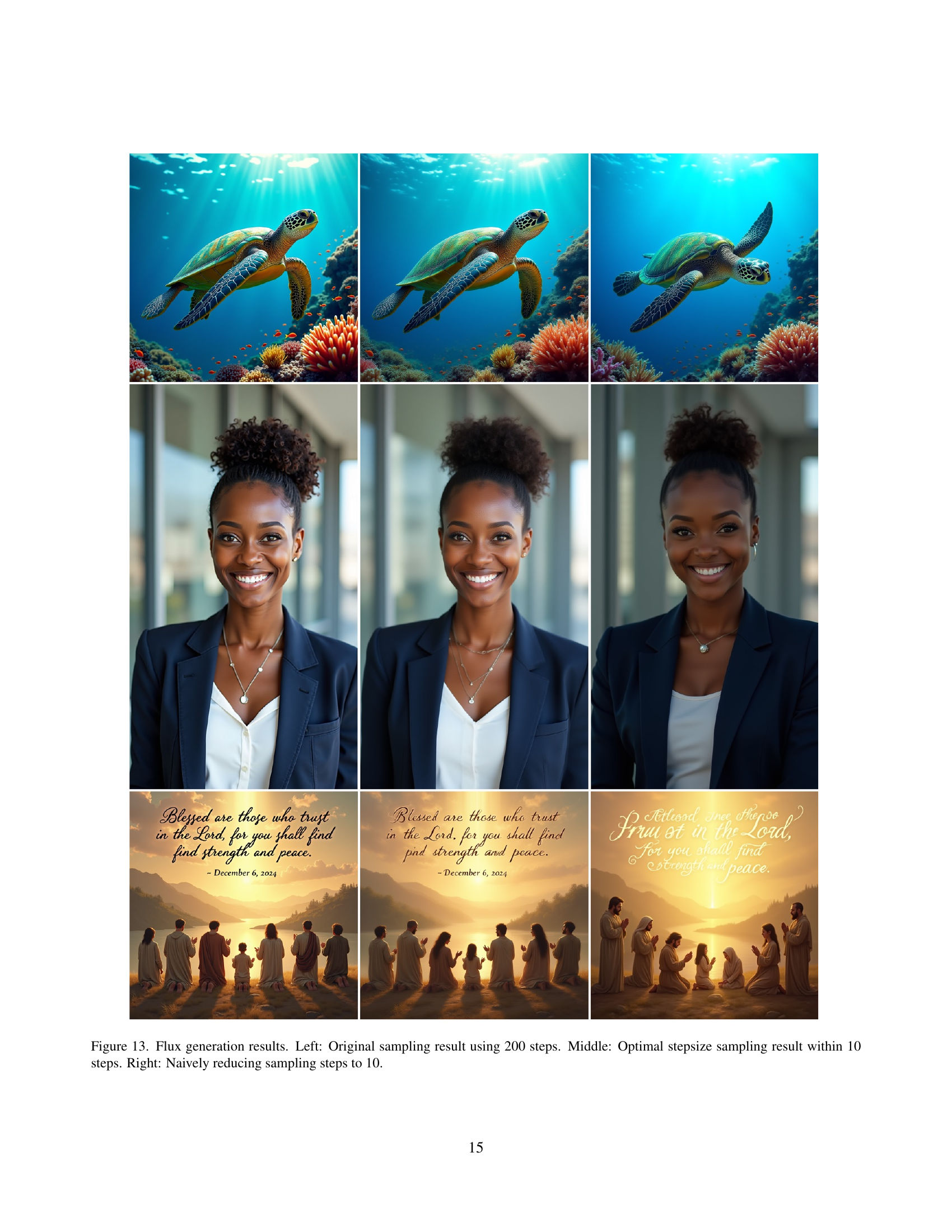
🔼 This figure demonstrates the impact of different sampling strategies on the quality of image generation using the Flux model. The leftmost image shows the result of the original sampling process using 200 steps. The center image displays the results using the optimized stepsize schedule proposed in this paper, achieving comparable quality with only 10 steps. The rightmost image shows what happens when the number of steps is naively reduced to 10 without optimization, resulting in a significant degradation of image quality.
read the caption
Figure 13: Flux generation results. Left: Original sampling result using 200 steps. Middle: Optimal stepsize sampling result within 10 steps. Right: Naively reducing sampling steps to 10.
More on tables
| steps | EDM | DDIM | FM | |
|---|---|---|---|---|
| Naive step reduction | 50 | 33.71 | 34.31 | 31.78 |
| 20 | 25.76 | 26.12 | 23.97 | |
| 10 | 20.83 | 20.89 | 19.00 | |
| 5 | 16.38 | 15.96 | 15.69 | |
| OSS | 20 | 28.21(+2.45) | 28.07(+1.95) | 28.51(+4.54) |
| 10 | 22.88(+2.05) | 22.79(+1.9) | 23.02(+4.02) | |
| 5 | 18.41(+2.03) | 18.05(+2.09) | 18.53(+2.84) |
🔼 This table presents the results of conditional image generation experiments on the ImageNet-64 dataset using different teacher noise schedules (EDM, DDIM, and Flow Matching). For each teacher schedule, a 200-step teacher model generated reference images. Then, student models were trained using the optimal stepsize distillation method (OSS) to generate images with 20, 10, and 5 steps. The table shows the Peak Signal-to-Noise Ratio (PSNR) between the student-generated images and the corresponding 200-step teacher images for each condition, demonstrating the robustness of the OSS method across different noise schedules. A naive step reduction baseline is included for comparison.
read the caption
Table 2: ImageNet-64 pixel space conditional image generation with different teacher schedules. All the student solvers are learned from the corresponding 200-step teacher schedule. Results are shown in PSNR calculated with 200-step corresponding teacher results.
| Teacher steps | 100 | 200 | 500 | 800 | 1000 |
|---|---|---|---|---|---|
| DDIM teacher | 37.97 | 44.24 | 52.93 | 57.30 | - |
| OSS | 27.04 | 28.07 | 27.11 | 27.12 | 27.13 |
| OSS-ave | 26.41 | 26.47 | 26.47 | 26.48 | 26.48 |
🔼 This table presents the results of conditional image generation on ImageNet-64 dataset using different numbers of steps in the teacher model during training. The teacher model consistently used the DDIM schedule. The student model always used 20 steps for inference. The performance metric used is PSNR, calculated by comparing the results of the student model to the results of a 1000-step teacher model. The goal is to illustrate the robustness of the proposed method across varying training conditions.
read the caption
Table 3: ImageNet-64 pixel space conditional image generation results with different teacher steps. All the teacher solver leverages DDIM schedules. Students adopt 20-steps for inference. Results are shown in PSNR calculated with the 1000-step teacher.
| -MSE | -MSE | -IncepV3 | -percep | |
|---|---|---|---|---|
| PSNR | 18.54 | 22.45 | 9.91 | 18.27 |
🔼 This table presents ablation study results, comparing the performance of different functions used to calculate the distance between the teacher and student models during the optimization process. The functions include Mean Squared Error (MSE) on the reparameterized clean data (x0-MSE), MSE on the intermediate feature xt (xt-MSE), Inception-V3 perceptual distance, and perceptual distance using the denoising network. The table shows the PSNR values achieved by each function, providing insight into their relative effectiveness in guiding the optimization of the student model’s trajectory to match that of the teacher model.
read the caption
Table 4: Ablation studies on different functions.
| w/o training | w training | |
|---|---|---|
| Uniform | 52.73 | 24.53 |
| OSS | 41.96 | 7.89 |
🔼 This table presents a comparison of FID scores achieved by various diffusion sampling methods on the ImageNet-256 dataset. The methods include: DDIM (using a uniform stepsize schedule), OSS (Optimal Stepsize), OSS-ave (a variant of OSS which averages results from 512 runs to improve consistency), and a baseline without training. The FID (Fréchet Inception Distance) scores quantify the quality of generated images, with lower scores indicating better image quality. The table allows for an assessment of the impact of different stepsize scheduling approaches, in particular OSS, on the performance of image generation.
read the caption
Table 5: Sampling results on ImageNet-256. Uniform is the schedule adopted in DDIM.
| Method | 5steps | 10steps | 5steps | 10steps |
|---|---|---|---|---|
| ImageNet-64 [24] | LSUN-Bed-256 [37] | |||
| EDM | 17.72 | 22.33 | 15.60 | 19.61 |
| DDIM | 17.69 | 22.22 | 15.39 | 20.18 |
| FM | 17.80 | 22.47 | 14.43 | 18.23 |
| DM | 17.39 | 20.50 | 18.90 | 20.67 |
| GITS | 16.29 | 19.40 | 11.58 | 13.55 |
| OSS-ave | 17.94 | 22.47 | 16.51 | 21.25 |
| FFHQ-64 [9] | MSCOCO-512 [14] | |||
| EDM | 18.68 | 23.24 | 13.43 | 15.45 |
| DDIM | 18.37 | 23.57 | 12.31 | 14.58 |
| FM | 17.72 | 21.31 | 11.90 | 13.51 |
| DM | 19.79 | 22.69 | 13.50 | 14.73 |
| GITS | 20.46 | 25.20 | 10.60 | 11.07 |
| OSS-ave | 20.56 | 25.21 | 14.10 | 16.45 |
🔼 Table 6 presents Peak Signal-to-Noise Ratio (PSNR) values, a metric for evaluating image quality, obtained using different stepsize schedules in diffusion models. The table compares the performance of various methods, including EDM, DDIM, FM, DM, GITS, and the proposed OSS-ave method. Each method’s PSNR is reported across multiple datasets (FFHQ-64 and MSCOCO-512) and with varying numbers of sampling steps (5 and 10). This allows for a comprehensive comparison of the efficiency and image quality achieved by each stepsize strategy.
read the caption
Table 6: PSNR results of different stepsize schedules.
| Method | steps | Overall |
|
| Counting | Colors | Position |
| ||||||
|---|---|---|---|---|---|---|---|---|---|---|---|---|---|---|
| Flow matching | 100 | 0.649 | 0.989 | 0.803 | 0.722 | 0.774 | 0.220 | 0.390 | ||||||
| Flow matching | 10 | 0.590 | 0.963 | 0.727 | 0.663 | 0.668 | 0.213 | 0.310 | ||||||
| DDIM | 10 | 0.623 | 0.971 | 0.742 | 0.694 | 0.758 | 0.22 | 0.353 | ||||||
| GITS | 10 | 0.604 | 0.981 | 0.732 | 0.678 | 0.697 | 0.210 | 0.325 | ||||||
| DM | 10 | 0.643 | 0.971 | 0.788 | 0.719 | 0.777 | 0.188 | 0.415 | ||||||
| OSS-ave | 10 | 0.645 | 0.981 | 0.775 | 0.728 | 0.777 | 0.195 | 0.415 |
🔼 This table presents the quantitative results of the GenEval benchmark using the Flux.1-dev model under different sampling schedules. It compares the performance of various sampling methods (Flow Matching, DDIM, GITS, DM, and the proposed OSS-ave) across various tasks (Overall, Counting objects, Two objects, Counting Colors, Position, Color attribution) using 10 and 100 steps. This allows for a comparison of the performance of different sampling strategies with varying numbers of steps, highlighting the efficiency and accuracy of the proposed method.
read the caption
Table 7: Results of Geneval based on the Flux.1-dev model with different sampling schedules.
Full paper#