↗ OpenReview ↗ NeurIPS Proc. ↗ Chat
TL;DR#
Graph Neural Networks (GNNs) are powerful tools for analyzing graph-structured data, but their expressive power is limited by the Weisfeiler-Leman (WL) test. Many GNNs struggle to effectively capture information about cycles and other complex substructures, hindering their performance on tasks requiring deep structural understanding. Existing higher-order WL variants offer increased expressivity but compromise on scalability, particularly with large, sparse graphs, common in real-world applications. This is problematic for many applications where the presence of specific substructures such as cycles is crucial.
This research introduces a novel approach called r-loopy Weisfeiler-Leman (r-lWL) and its corresponding GNN framework, r-loopy Message Passing Neural Network (r-lMPNN). The method enhances the expressive power of GNNs by incorporating information from paths of varying lengths between nodes. The key finding is that r-lWL can count cycles up to length r+2, surpassing existing WL hierarchies and even outperforming methods explicitly designed for cycle counting. This improved expressivity is demonstrated empirically on various real-world datasets, particularly sparse graphs, showing that r-lMPNN achieves competitive performance and maintains excellent scalability.
Key Takeaways#
Why does it matter?#
This paper is crucial because it presents r-lWL, a novel graph isomorphism test hierarchy, and its corresponding GNN framework, r-lMPNN. These advancements are significant for researchers tackling challenges in graph neural networks (GNNs), particularly those focused on expressive power and scalability. The framework extends existing methods by enabling the counting of cycles and homomorphisms of cactus graphs, offering a robust solution for analyzing complex graph structures. It is important for understanding the limitations of existing GNNs and for developing novel expressive GNNs.
Visual Insights#
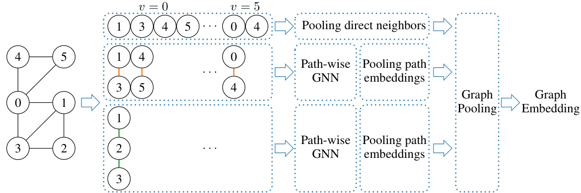
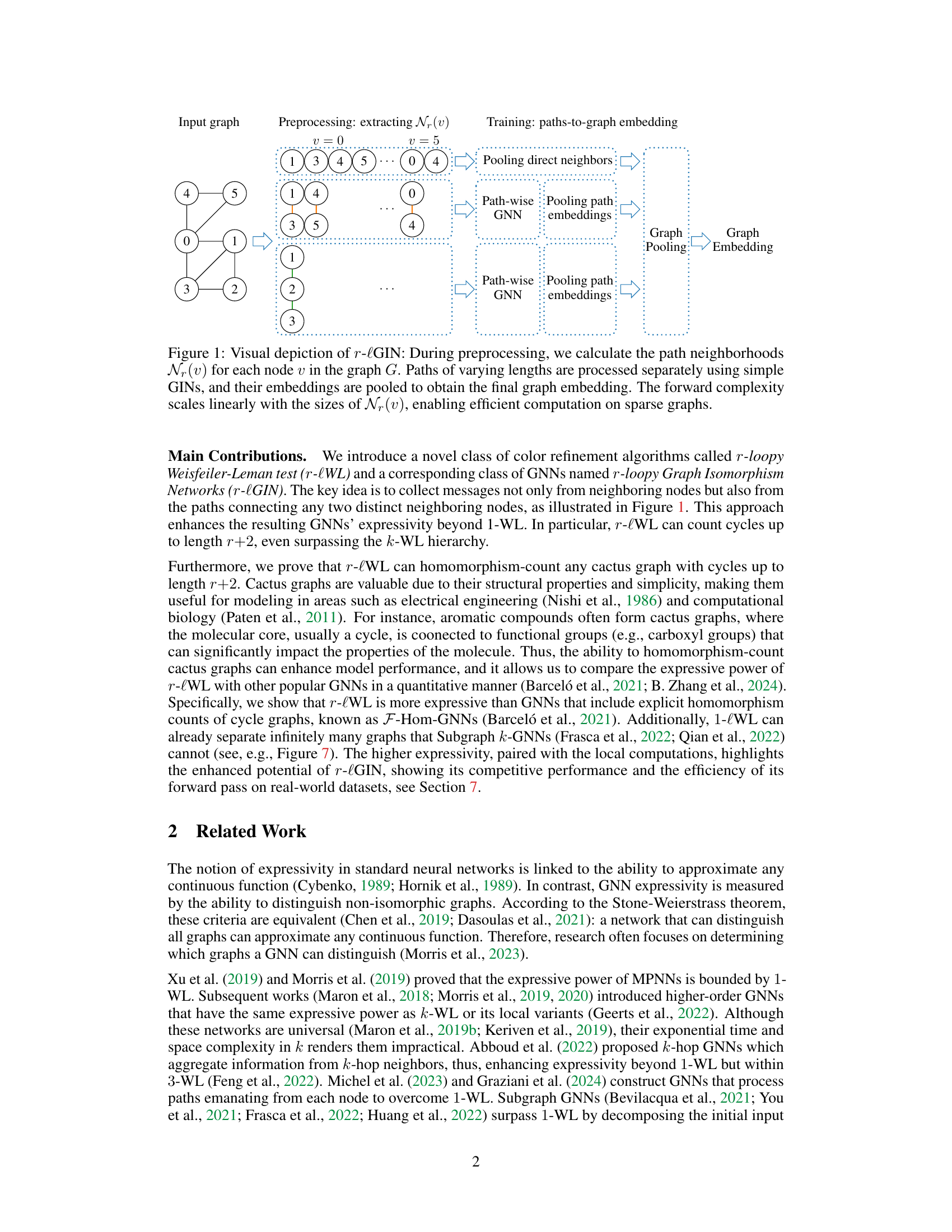
This figure shows the architecture of r-lGIN, a graph neural network (GNN) based on the r-loopy Weisfeiler-Leman test. The input is a graph. The preprocessing step extracts the r-neighborhoods for each node, which are collections of paths of length up to r connecting neighbors of the node. These paths are processed by separate graph isomorphism networks (GINs), and their embeddings are pooled together to create a node embedding. Node embeddings are then pooled to create a graph embedding. The process is designed to be computationally efficient, especially for sparse graphs, as the complexity scales linearly with the size of the r-neighborhoods.
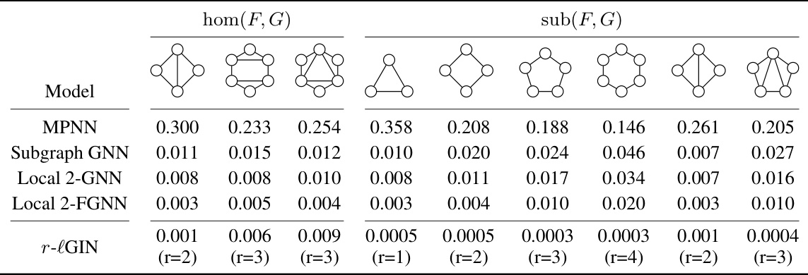
This table compares the performance of various graph neural network models (MPNN, Subgraph GNN, Local 2-GNN, Local 2-FGNN, and r-lGIN) on the SUBGRAPHCOUNT dataset. The models are evaluated based on their ability to accurately predict homomorphism counts (hom(F, G)) and subgraph counts (sub(F, G)) for different motifs (F). Lower values in the table indicate better performance. The r-lGIN model shows significantly better performance than other models, demonstrating its effectiveness in subgraph counting.
In-depth insights#
Loopy WL Hierarchy#
The hypothetical “Loopy WL Hierarchy” in graph neural networks (GNNs) suggests a refinement of the Weisfeiler-Leman (WL) test, a fundamental algorithm for graph isomorphism testing. A standard WL test iteratively refines node colors based on the colors of their neighbors. A “loopy” variant might extend this by incorporating information from paths of various lengths between neighbors, going beyond the purely local neighborhood information of the standard WL test. This could significantly enhance the expressive power of GNNs. The hierarchical aspect implies a series of increasingly powerful loopy WL tests, potentially leading to a hierarchy that interleaves or surpasses existing k-WL tests. The key advantage is the potential to capture more global graph structure while maintaining a degree of computational efficiency. However, the tradeoff between expressive power and computational cost needs careful study. Scalability issues could arise as path lengths increase, particularly for large or dense graphs. Therefore, efficient implementation strategies are crucial for practical application.
r-lMPNN: A GNN#
The heading “r-lMPNN: A GNN” suggests a novel Graph Neural Network (GNN) architecture. The “r-l” prefix likely denotes a modification to standard MPNNs (Message Passing Neural Networks) that enhances their capabilities, possibly by incorporating information from paths of length ‘r’ in the graph. This implies a move beyond the limitations of 1-WL (Weisfeiler-Lehman) test, a common bottleneck for MPNN expressiveness. The enhanced expressivity might enable r-lMPNN to capture more complex graph features, leading to improved performance on tasks involving intricate relationships between nodes. The name also hints at scalability, a crucial aspect of GNNs, suggesting the architecture is designed to handle large and sparse graphs efficiently. Further details would be needed to understand its specific mechanism for path aggregation and the choice of ‘r’, but overall, r-lMPNN presents a promising development in GNN research, potentially offering a powerful tool for tasks requiring high expressivity and efficient computation.
Expressiveness: r-lWL#
The heading ‘Expressiveness: r-lWL’ suggests an analysis of the expressive power of the r-loopy Weisfeiler-Leman (r-lWL) algorithm, a novel graph isomorphism test. The core argument likely centers on how r-lWL’s ability to count cycles up to a certain length impacts its capacity to distinguish non-isomorphic graphs. A key aspect would be demonstrating that r-lWL surpasses the limitations of the standard 1-WL test, which struggles to differentiate graphs with subtle structural variations. The discussion likely involves a theoretical analysis, possibly proving that r-lWL can count specific graph substructures (homomorphisms) that 1-WL cannot. Empirical results would probably be included to showcase r-lWL’s improved ability to discriminate between graphs on benchmark datasets. The overall goal would be to establish a hierarchy showing how the expressive power of r-lWL increases with the parameter ‘r’, demonstrating a significant enhancement over existing methods for graph representation learning.
Scalability and Limits#
A discussion on “Scalability and Limits” in a research paper would explore the practical constraints of the proposed method. It would address how well the approach handles large datasets and complex graphs, analyzing computational cost and memory usage. Scalability is crucial, as the method’s usefulness depends on its ability to be deployed in real-world scenarios. The discussion should also identify the inherent limitations of the model; what types of problems it cannot solve or where its performance significantly degrades. It’s important to acknowledge the trade-offs between expressiveness and efficiency. For instance, a highly expressive model might lack scalability, while a fast model may struggle with complex data structures. This section should present a balanced perspective, presenting both successes and limitations to provide a realistic assessment of the method’s overall viability.
Future Work#
Future research directions stemming from this Weisfeiler-Leman extension could involve analyzing the maximal class of graphs homomorphism-countable by r-lWL, potentially clarifying its precise expressive power compared to other WL variants and GNNs. This would entail identifying graph families that are separable by r-lWL but not by other methods, leading to a more precise categorization of graph isomorphism problems. Another promising avenue is exploring the generalization capabilities of GNNs with provable homomorphism-counting properties. The capacity to count specific motifs could offer a robust mathematical framework to support the intuitive notion that counting relevant structural features might significantly boost a GNN’s generalization performance. Finally, investigating the scalability of r-lWL for larger and denser graphs is crucial. While showing efficacy on sparse datasets, applying the method to real-world dense graph instances requires further study and the development of optimized algorithms to enhance computational efficiency. Therefore, future work should focus on addressing these crucial aspects to solidify the theoretical underpinnings and broaden the practical applicability of this new graph neural network architecture.
More visual insights#
More on figures
This figure illustrates the architecture of the r-loopy Graph Isomorphism Network (r-lGIN). The input graph undergoes preprocessing where path neighborhoods of varying lengths (r-neighborhoods) are calculated for each node. These paths are then processed independently by using simple Graph Isomorphism Networks (GINs). The resulting embeddings are pooled together to create a final graph embedding. The linear scaling of the forward complexity with the size of r-neighborhoods ensures the efficiency of the model, particularly for sparse graphs.

This figure shows the results of an experiment testing the expressive power of the r-lGIN model. Four different datasets (GRAPH8C, EXP_ISO, COSPECTRAL10, SR16622) are used to compare the ability of the model to distinguish between pairs of graphs that are considered indistinguishable by other methods. The x-axis represents the proportion of indistinguishable pairs or the L¹ distance between graph embeddings (depending on the dataset), and the y-axis shows the parameter ‘r’ used in the r-lGIN model. The plot visually demonstrates how increasing ‘r’ improves the model’s ability to distinguish between non-isomorphic graphs.
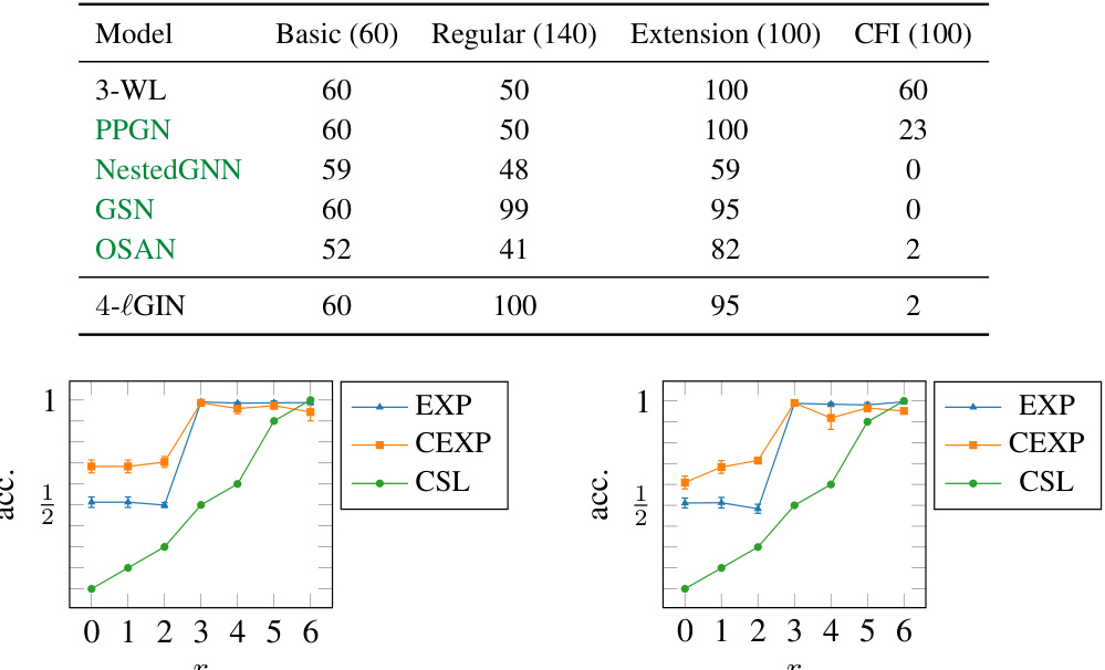
The figure shows the test accuracy on three synthetic classification tasks (EXP, CEXP, CSL) with different values of (r). The left panel shows results when the weights are shared among all (r) values, while the right panel shows results when the weights are not shared. The results demonstrate that increasing (r) generally improves test accuracy, especially with non-shared weights. This highlights the benefit of the proposed r-lGIN architecture in capturing higher-order structural information in graphs.
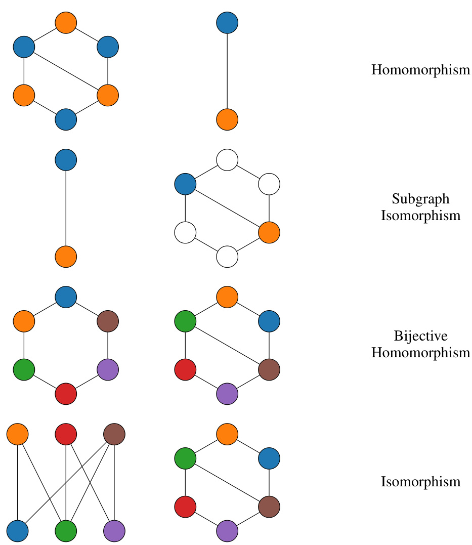
This figure shows four rows of graph pairs, illustrating the differences between homomorphism, subgraph isomorphism, bijective homomorphism and isomorphism. The mappings between the graphs are visually represented with colors for clarity. In each row, the graph on the left is consistently F and the one on the right G. Row 1 shows a non-injective homomorphism. Row 2 is a subgraph isomorphism, indicating that F is a subgraph of G. Row 3 presents a bijective homomorphism with a non-homomorphic inverse, while the final row illustrates isomorphism where the graphs are identical.
This figure shows a visual representation of the r-loopy Graph Isomorphism Networks (r-lGIN) architecture. The preprocessing step involves calculating the path neighborhoods (Nr(v)) for each node in the input graph. These paths, of varying lengths, are processed independently using Graph Isomorphism Networks (GINs). The resulting embeddings are then pooled together to create a final graph embedding. The architecture is designed for efficiency with sparse graphs because the forward pass scales linearly with the size of the path neighborhoods.
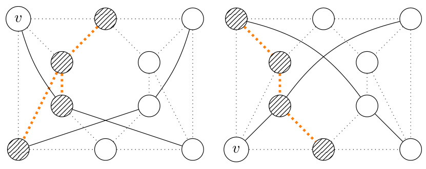
The figure shows two graphs that cannot be distinguished by r-lWL but can be distinguished by (r+1)-lWL. The graph on the left is a chordal cycle, while the graph on the right is a cactus graph. This illustrates that the expressiveness of r-lWL increases with r.
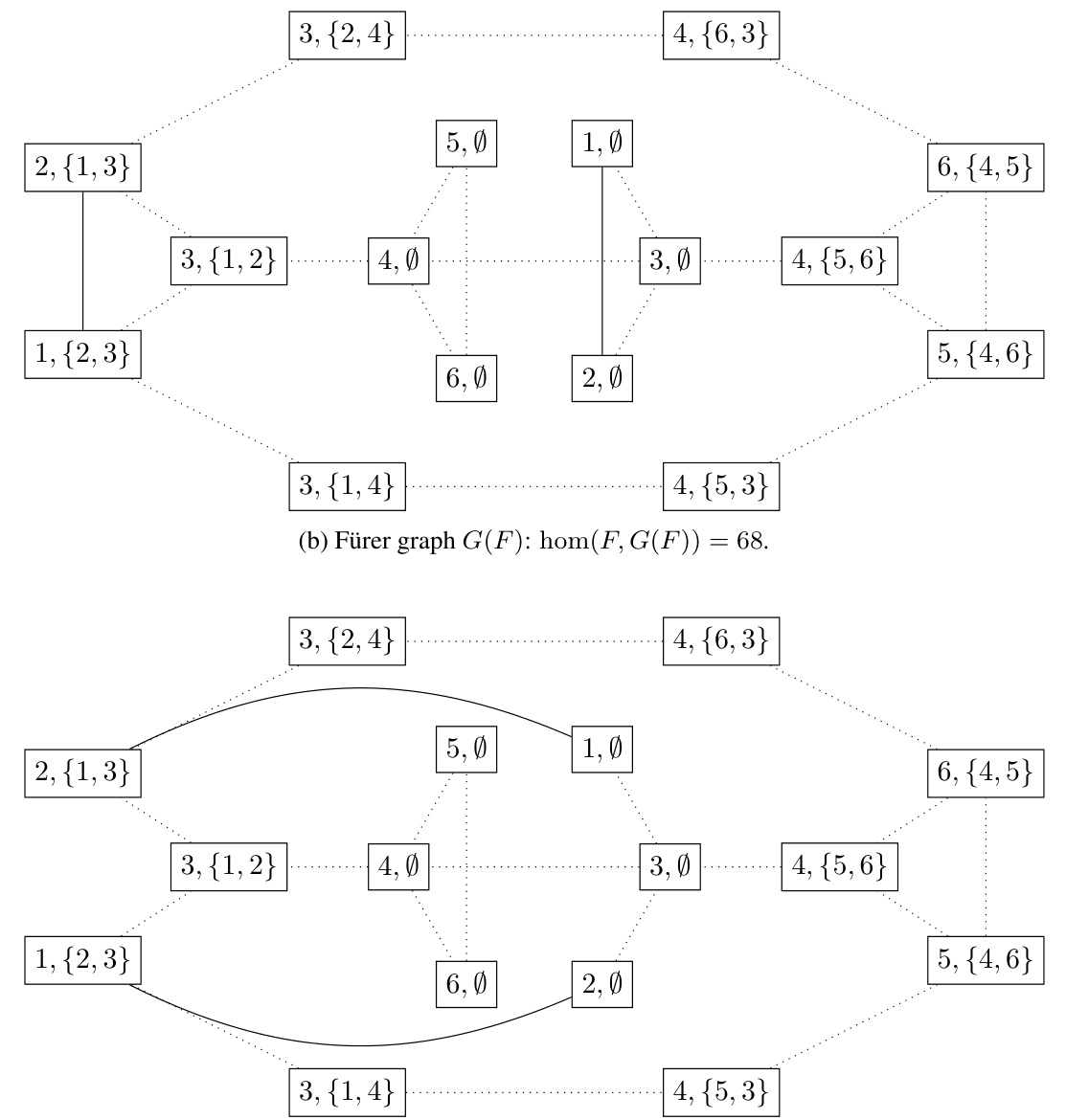
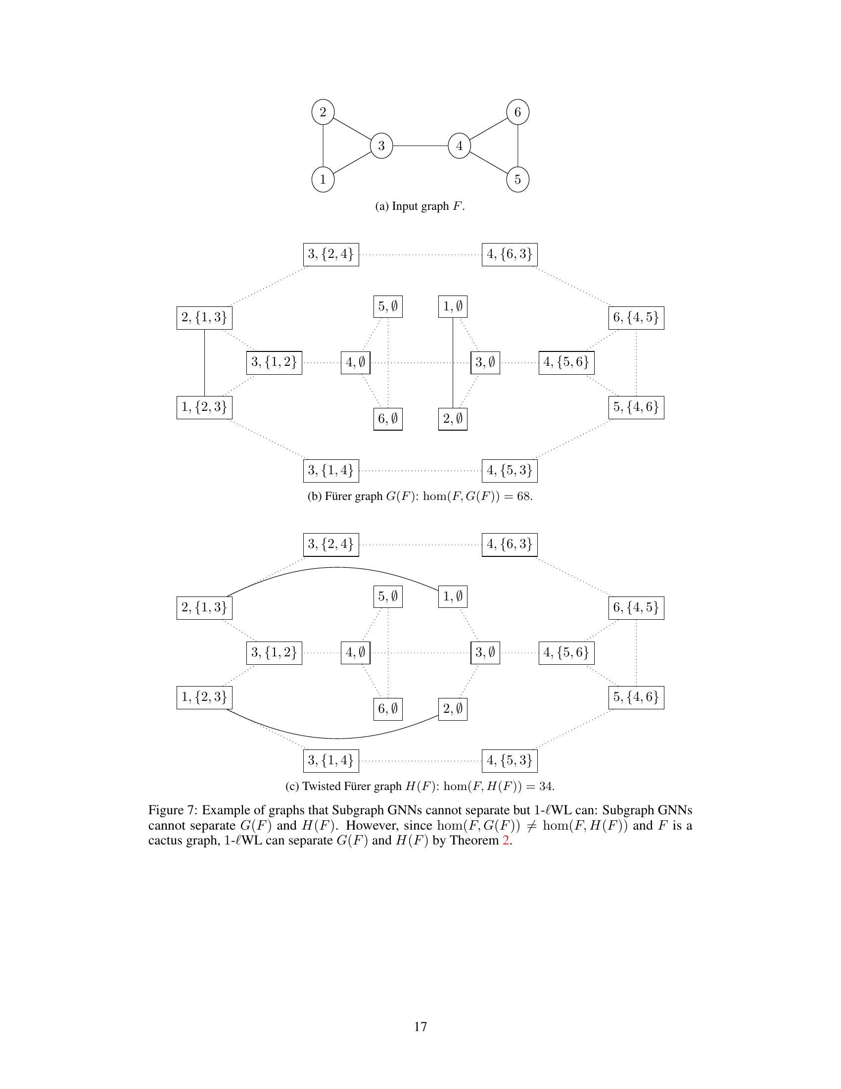
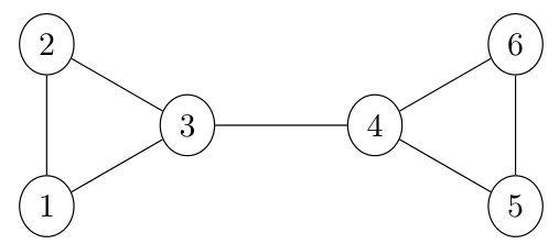
The figure shows three graphs. Graph (a) is the input graph F. Graphs (b) and (c) are G(F) and H(F) which are obtained by applying Fürer graph construction on the input graph F. These graphs can not be separated by Subgraph GNNs, but can be separated by 1-lWL because their homomorphism counts of the input graph F are different.
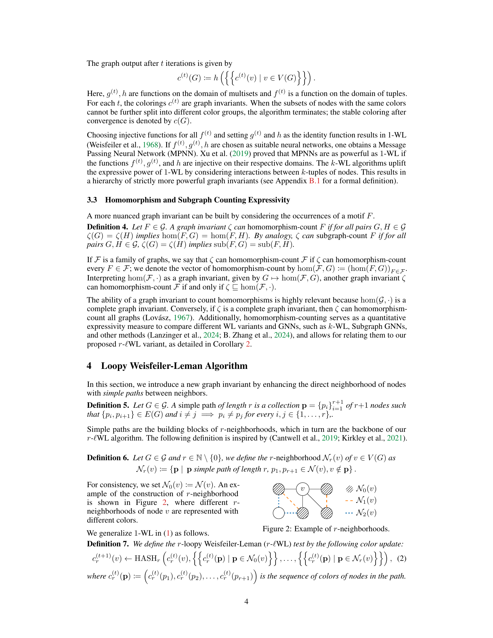
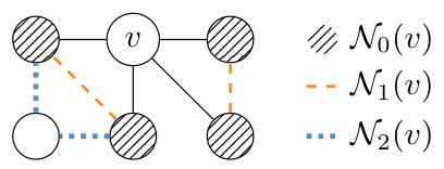
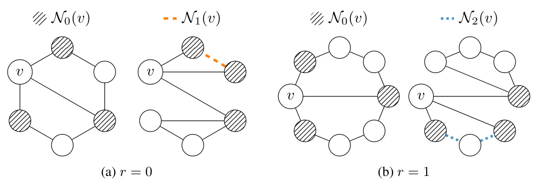
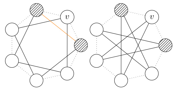
This figure visually depicts the concept of r-neighborhoods (Nr(v)) around a node ‘v’ in a graph. N0(v) represents the immediate neighbors of ‘v’. As ‘r’ increases, Nr(v) includes paths of length ‘r’ connecting pairs of nodes in N0(v), without including node ‘v’ itself in the path. Different colors highlight the distinct r-neighborhoods for different values of r, showing how the neighborhood expands with increasing path lengths.
The figure shows an example of how r-neighborhoods are constructed around a central node (v). For r=0, the neighborhood includes only directly connected nodes. As r increases, the neighborhood expands to include nodes connected by paths of length r, where each path starts and ends with a node directly connected to the central node. Different colors are used to visually distinguish the r-neighborhoods for different values of r.
The figure shows two graphs that cannot be distinguished by the r-loopy Weisfeiler-Leman (r-lWL) test but can be distinguished by the (r+1)-lWL test. The left graph is a cycle with a chord added, while the right graph is a cactus graph (a graph where every edge belongs to at most one cycle). This illustrates that increasing the parameter ‘r’ in the r-lWL test increases its ability to distinguish non-isomorphic graphs.
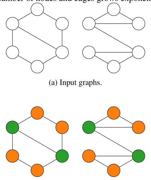
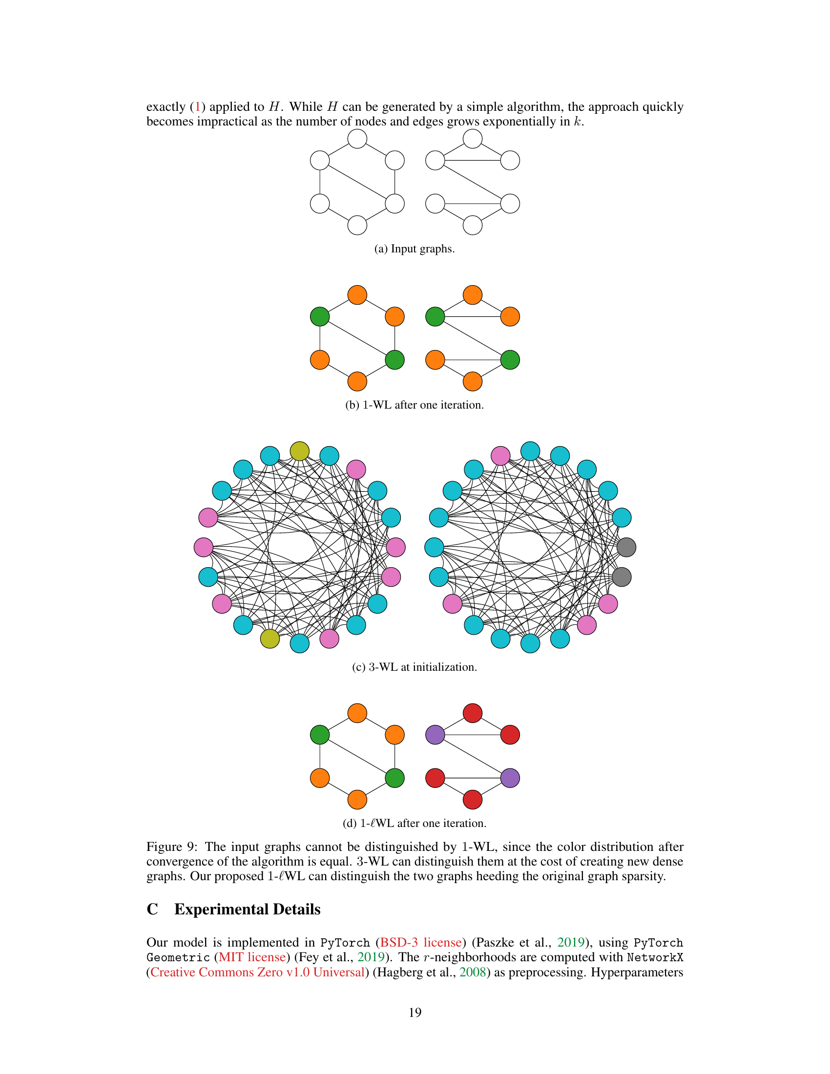
This figure shows two graphs that cannot be distinguished by the 1-WL test because they have the same color distribution after convergence. However, the 3-WL test can distinguish them but at the cost of creating new dense graphs. The proposed 1-lWL test can distinguish these graphs while preserving the original graph sparsity, demonstrating its advantage.
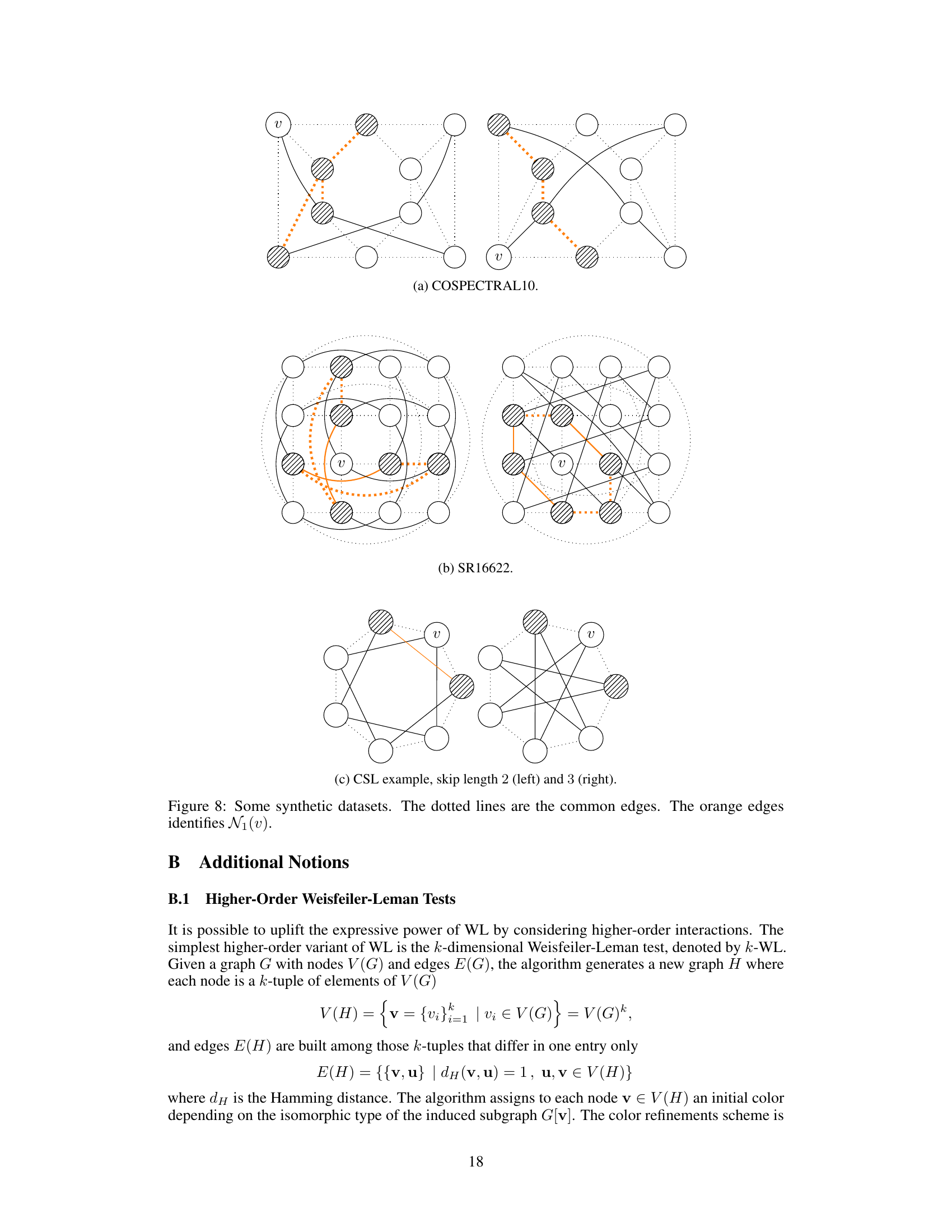
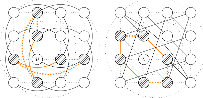
This figure shows three examples of synthetic datasets used to evaluate the expressive power of the proposed r-lGIN model. The datasets are COSPECTRAL10, SR16622, and CSL, each designed to test the model’s ability to distinguish graphs with subtle structural differences. In each example, the graphs share a common core structure (represented by dotted lines), but differ in the additional edges connecting nodes. The orange edges highlight the 1-neighborhoods of a selected node (v). This visualizes the paths of length up to r that are considered by the r-lWL algorithm. The aim is to illustrate the enhanced expressiveness of the proposed model beyond the limitations of the standard Weisfeiler-Leman test.
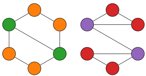
This figure shows four rows of examples demonstrating different types of mappings between two graphs, F and G, which are represented by different colors for their nodes. The mappings illustrate the differences between homomorphism, subgraph isomorphism, bijective homomorphism with non-homomorphic inverse, and isomorphism.

The figure shows an example of how r-neighborhoods are constructed for a given node in a graph. For r=0, the neighborhood is simply the set of direct neighbors. For r=1, the r-neighborhood includes paths of length 1 between any two direct neighbors. For r=2, the r-neighborhood includes paths of length 2 between any two direct neighbors.

This figure shows the architecture of the r-loopy Graph Isomorphism Network (r-lGIN). The input is a graph. The preprocessing step extracts the r-neighborhoods for each node, which are sets of paths of length r starting from that node and ending in its neighbors. These paths are processed independently using Graph Isomorphism Networks (GINs), and their embeddings are pooled together to create the final graph embedding. The linear scaling of the forward complexity with the size of the r-neighborhoods is a key advantage of this method.

This figure shows an example where Subgraph GNNs fail to distinguish between two graphs, G(F) and H(F), while the 1-loopy Weisfeiler-Leman (1-lWL) test can. The graphs G(F) and H(F) are constructed from a base graph F. The key difference is that 1-lWL considers paths between nodes, enabling it to distinguish the graphs based on their different homomorphism counts (hom(F,G(F)) and hom(F,H(F))). This illustrates the increased expressive power of 1-lWL over Subgraph GNNs.
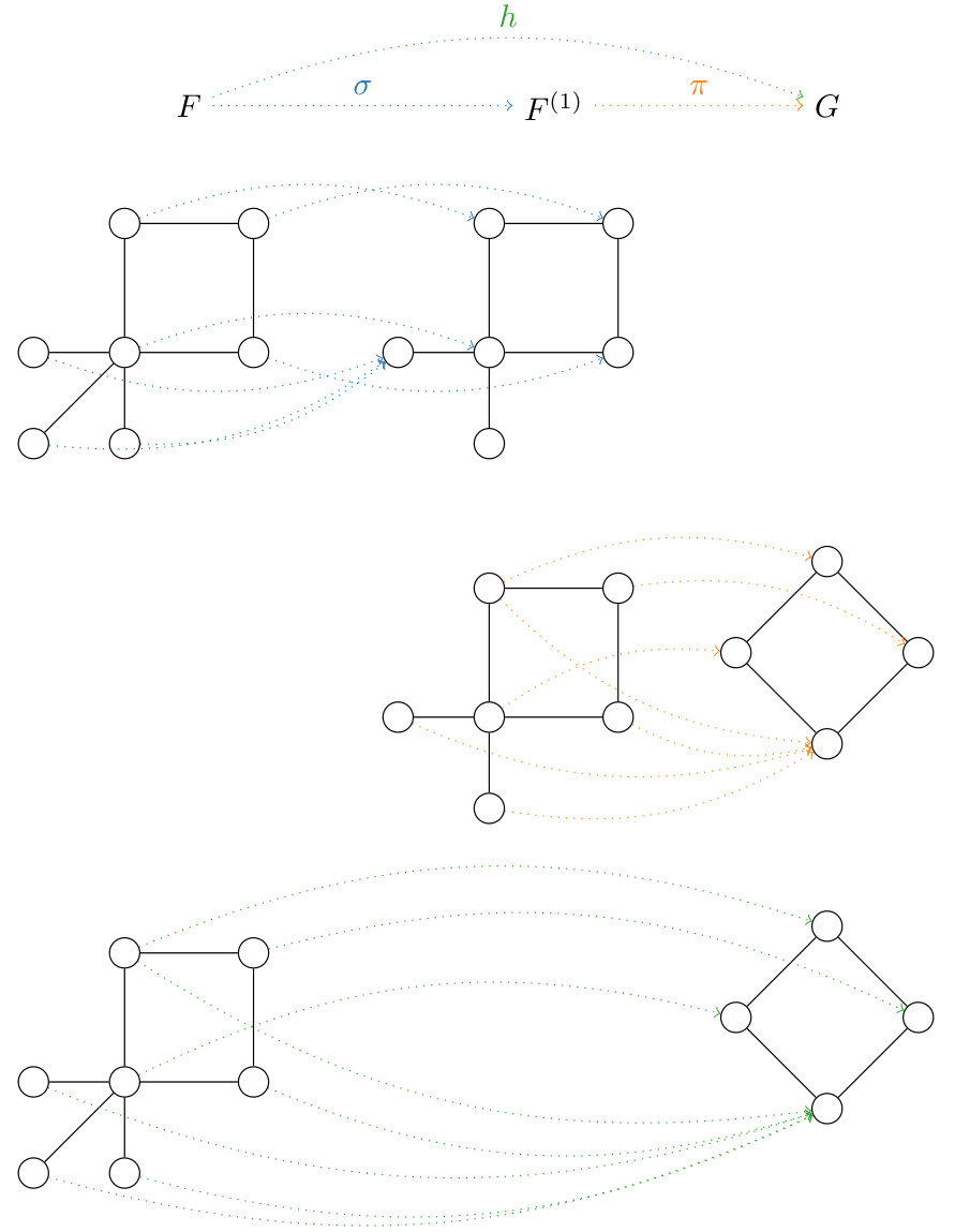
This figure illustrates four different types of mappings between two graphs, F and G. Each row demonstrates a different type of mapping: non-injective homomorphism, subgraph isomorphism, bijective homomorphism (with non-homomorphic inverse), and isomorphism. The mappings are visually represented using colors for clarity.

This figure shows an example where the 1-loopy Weisfeiler-Leman test (1-lWL) can distinguish between two graphs that Subgraph GNNs cannot. It highlights the increased expressive power of 1-lWL, specifically in relation to counting homomorphisms of specific graph types (in this case, a cactus graph). The figure includes three subfigures: (a) an input graph F; (b) a Fürer graph G(F); and (c) a twisted Fürer graph H(F). Subgraph GNNs cannot distinguish between G(F) and H(F), whereas 1-lWL can due to their differing homomorphism counts. This demonstrates that 1-lWL is more powerful.

This figure shows two graphs that cannot be distinguished by the r-loopy Weisfeiler-Leman test (r-lWL), but can be distinguished by the (r+1)-lWL test. The left graph is a cycle graph with a chord, while the right graph is a cactus graph. This illustrates that increasing the value of ‘r’ in r-lWL increases its ability to distinguish non-isomorphic graphs.
More on tables
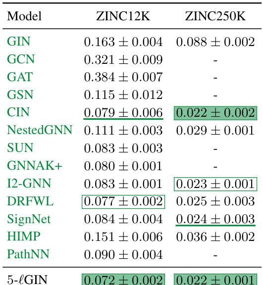
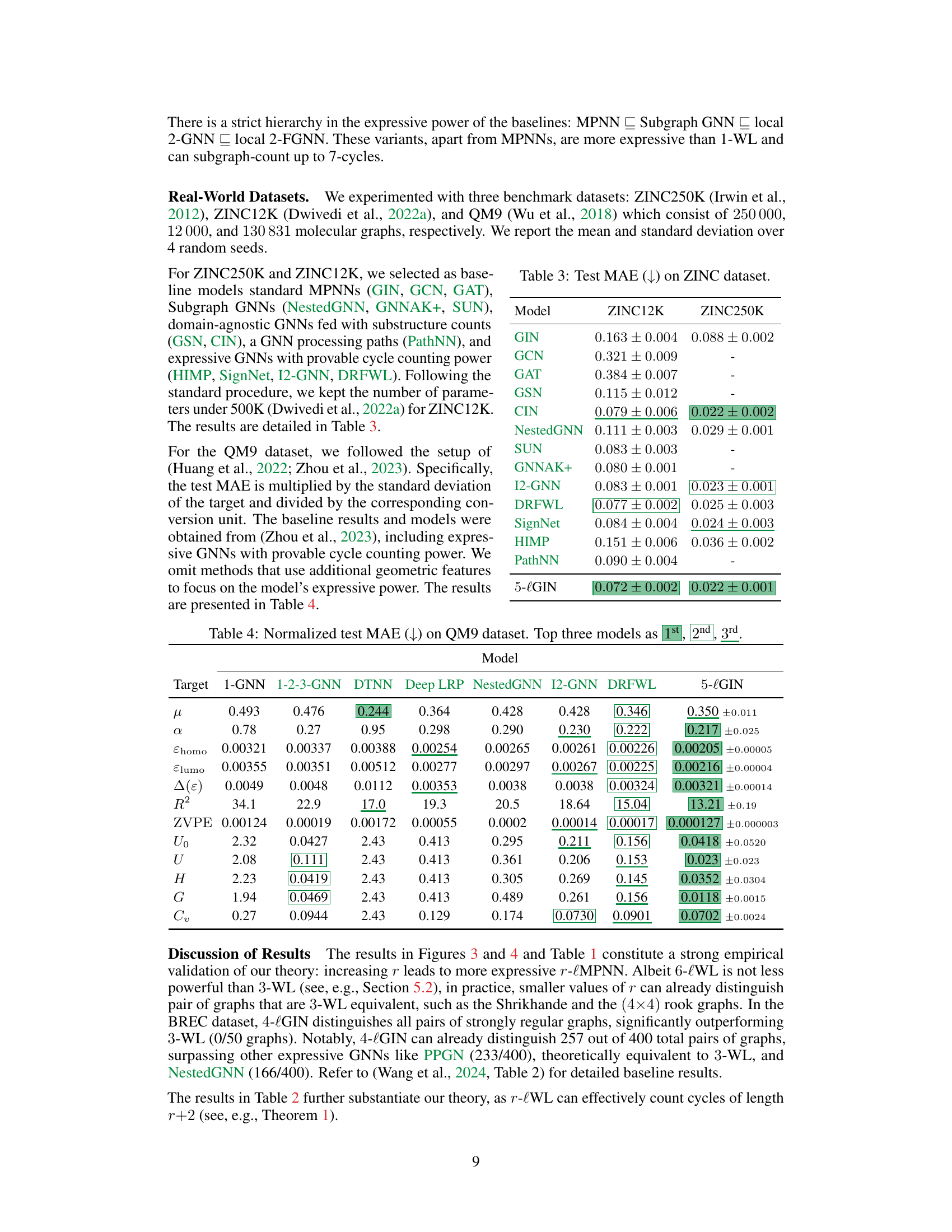
This table presents the Mean Absolute Error (MAE) achieved by various graph neural network models on the ZINC12K and ZINC250K datasets. Lower MAE indicates better performance. The models tested include standard MPNNs (GIN, GCN, GAT), Subgraph GNNs (NestedGNN, GNNAK+, SUN), domain-agnostic GNNs (GSN, CIN), a GNN processing paths (PathNN), and expressive GNNs with provable cycle-counting power (HIMP, SignNet, I2-GNN, DRFWL), as well as the proposed 5-lGIN. The results highlight the performance of 5-lGIN in comparison to other state-of-the-art models.
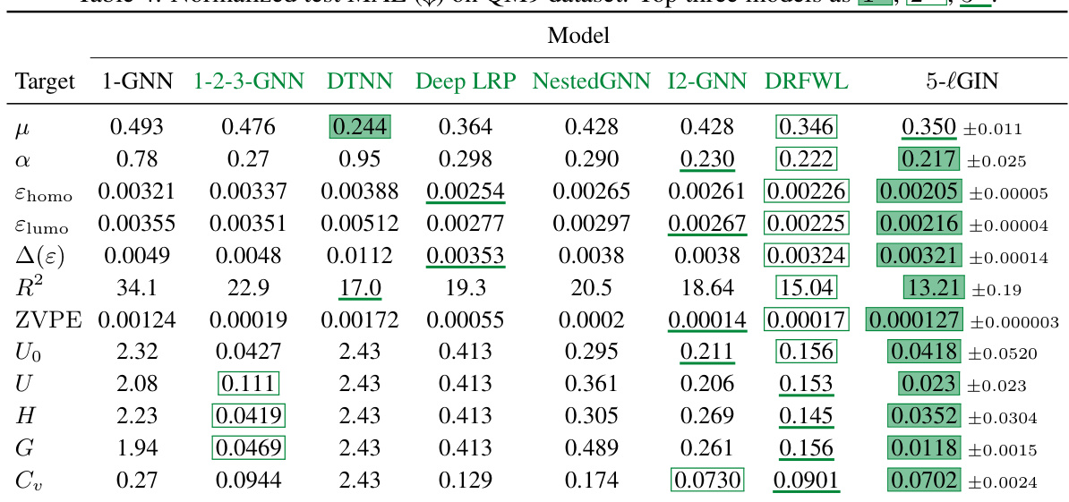
This table presents the normalized test mean absolute error (MAE) achieved by various models on the QM9 dataset. The MAE is a common metric to evaluate the performance of regression models, representing the average absolute difference between predicted and actual values. Lower MAE indicates better performance. The table compares the performance of 5-lGIN against other models, highlighting its performance relative to other approaches on various target properties.
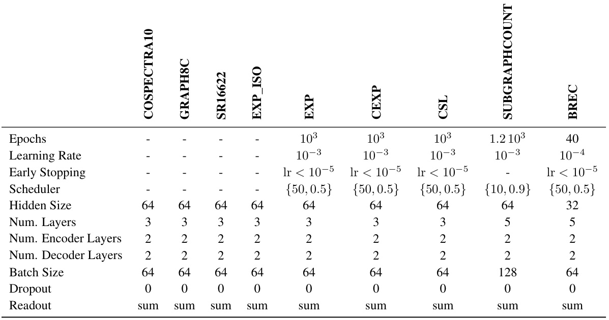
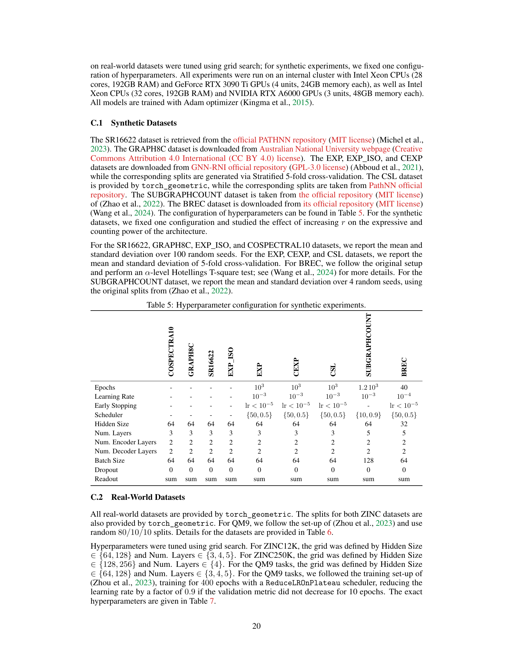
This table shows the hyperparameter settings used for the synthetic experiments in the paper. It lists the values used for various parameters, such as the number of epochs, learning rate, early stopping criteria, scheduler type, hidden size, number of layers (encoder and decoder), batch size, dropout rate, and readout method. These parameters were tuned for different synthetic datasets, namely GRAPH8C, EXP_ISO, COSPECTRAL10, SR16622, EXP, CEXP, CSL, SUBGRAPHCOUNT, and BREC. The values listed represent those used to generate the reported results for those datasets.
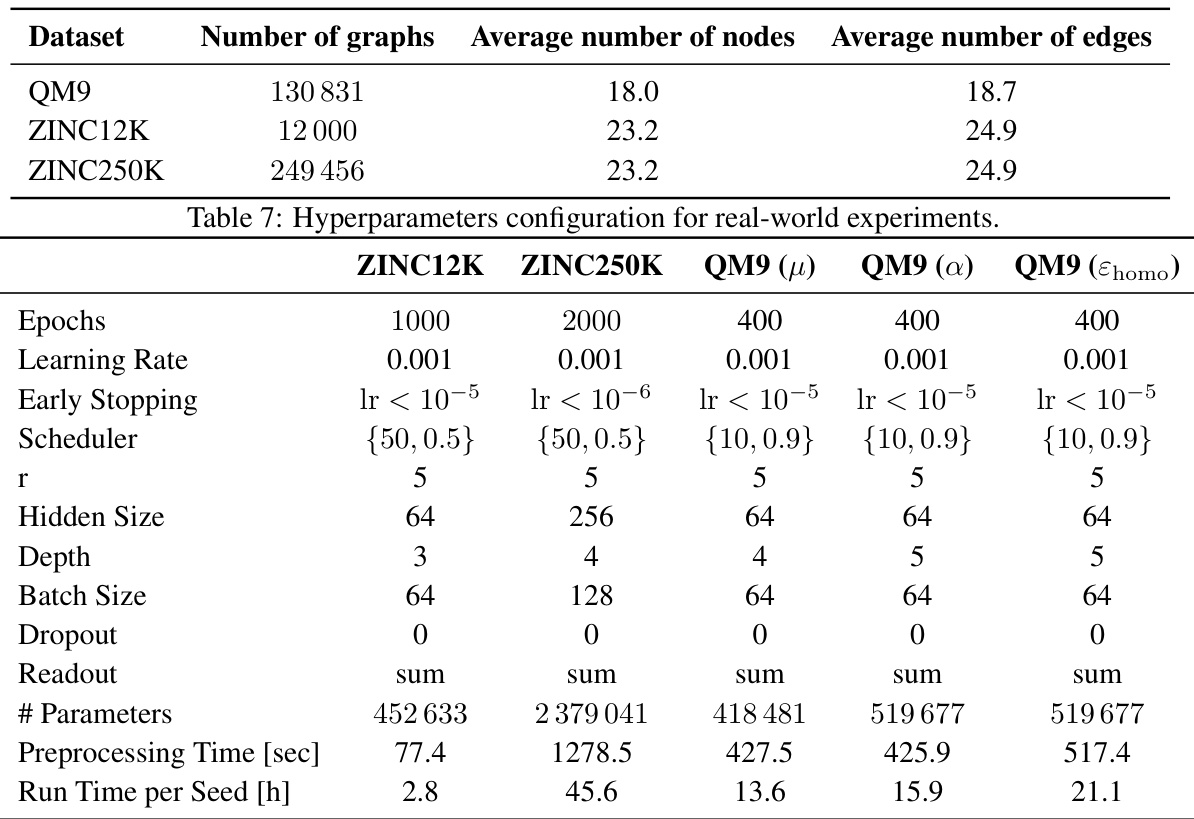
This table presents the hyperparameter settings used for the experiments conducted on real-world datasets. It includes the number of epochs, learning rate, early stopping criteria, learning rate scheduler, the value of the hyperparameter r, hidden size, depth of the network, batch size, dropout rate, readout method, total number of parameters, preprocessing time in seconds, and the run time per seed in hours. The specific hyperparameters varied across datasets to optimize performance, and the table indicates these variations for each dataset (ZINC12K, ZINC250K, and QM9 for different properties).
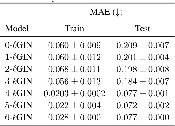
This table shows the ablation study on the effect of different values of the hyperparameter r on the performance of the r-lGIN model on the ZINC12K dataset. It demonstrates the impact of incorporating paths of varying lengths into the model’s architecture, showing how this affects both training and test performance as measured by Mean Absolute Error (MAE).
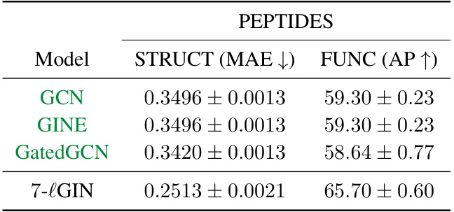
This table presents the results of experiments conducted on long-range graph benchmark datasets. It compares the performance of the proposed 7-lGIN model against several baseline models (GCN, GINE, GatedGCN) on two specific tasks: STRUCT (predicting structural properties) and FUNC (predicting functional properties). The metrics used are Mean Absolute Error (MAE) for STRUCT (lower is better) and Average Precision (AP) for FUNC (higher is better). The baseline results are taken from a previous study by Dwivedi et al. (2022b).
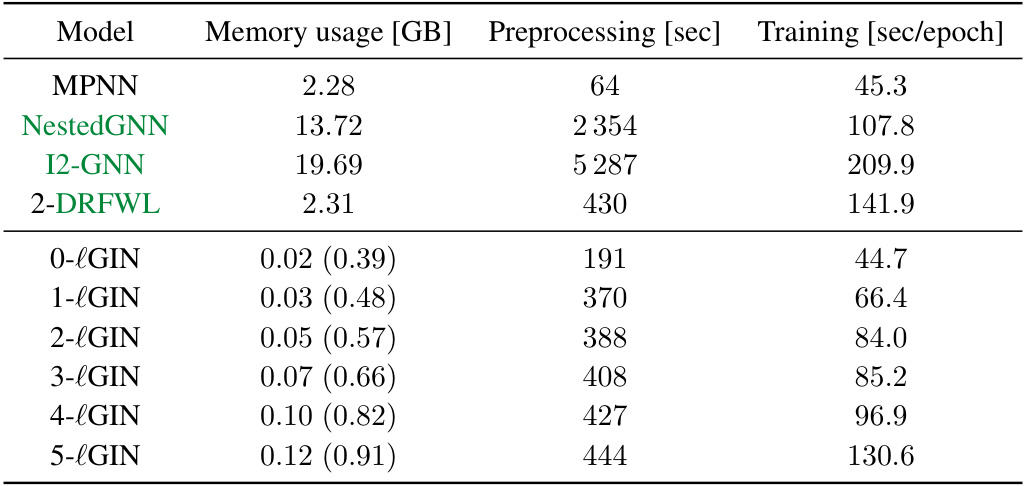
This table compares the memory usage, preprocessing time, and training time per epoch for different models on the QM9 dataset. It shows that the proposed r-lGIN models have relatively low memory usage and training time compared to other models, especially as the value of ‘r’ increases. The numbers in parentheses show the size of the dataset after the r-neighborhoods have been computed; this is relevant because computation of these neighborhoods is a preprocessing step, and the table shows that the size of this dataset does not increase dramatically with r.
Full paper#
