↗ OpenReview ↗ NeurIPS Proc. ↗ Chat
TL;DR#
Accurately solving the many-electron Schrödinger equation is fundamental to computational chemistry, but existing methods using Slater determinants are computationally expensive and lack generalizability. Additionally, enforcing electron antisymmetry remains challenging. These limitations hinder the accurate prediction of molecular properties for complex systems.
The paper introduces Neural Pfaffians, a novel method leveraging Pfaffians to define fully learnable neural wave functions. This approach overcomes the limitations of Slater determinants by lifting the constraints on orbital numbers and spin configurations. The proposed Neural Pfaffian model achieves chemical accuracy in various systems and significantly reduces energy errors compared to previous methods, demonstrating its superior accuracy and generalizability.
Key Takeaways#
Why does it matter?#
This paper is crucial for researchers in quantum chemistry and machine learning because it presents a novel approach to accurately and efficiently calculate the ground state energy of many-electron systems, a long-standing challenge in the field. The introduction of the Neural Pfaffian model, alongside its efficient implementation, opens new avenues for developing more accurate and generalizable wave functions, pushing the boundaries of computational chemistry.
Visual Insights#
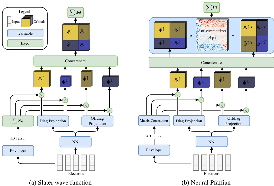
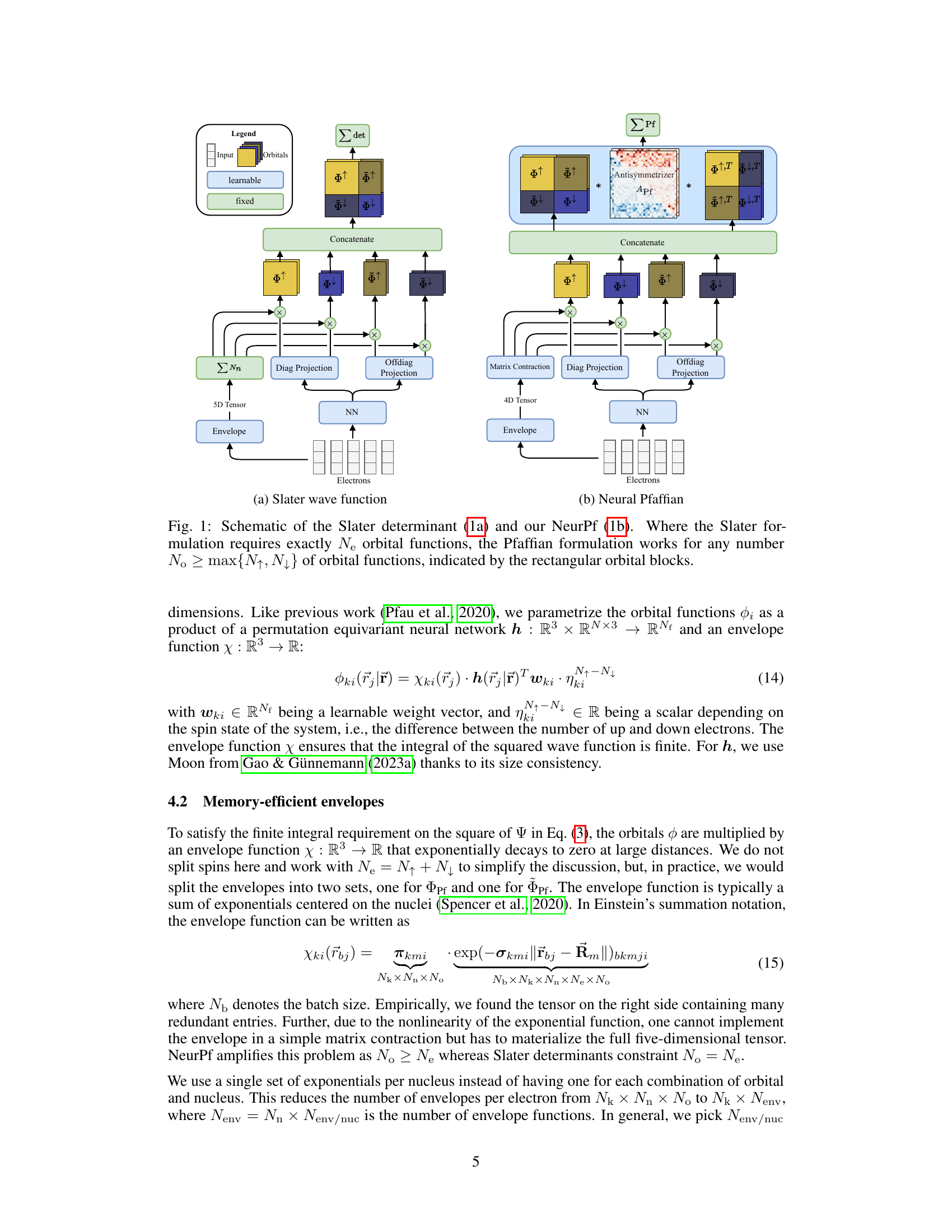
This figure illustrates the architectural differences between the traditional Slater determinant approach and the proposed Neural Pfaffian method for constructing electronic wave functions. The left panel (a) depicts the Slater determinant, which requires a square matrix of exactly Ne orbitals (where Ne is the total number of electrons), with separate orbitals for spin-up and spin-down electrons. The right panel (b) shows the Neural Pfaffian, which allows for an over-parameterized approach where the number of orbitals (No) can be greater than or equal to the maximum of N↑ and N↓ (the number of spin-up and spin-down electrons, respectively). This flexibility is achieved by utilizing a Pfaffian instead of a determinant, enabling a more general and potentially more accurate representation of the wave function.
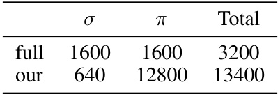
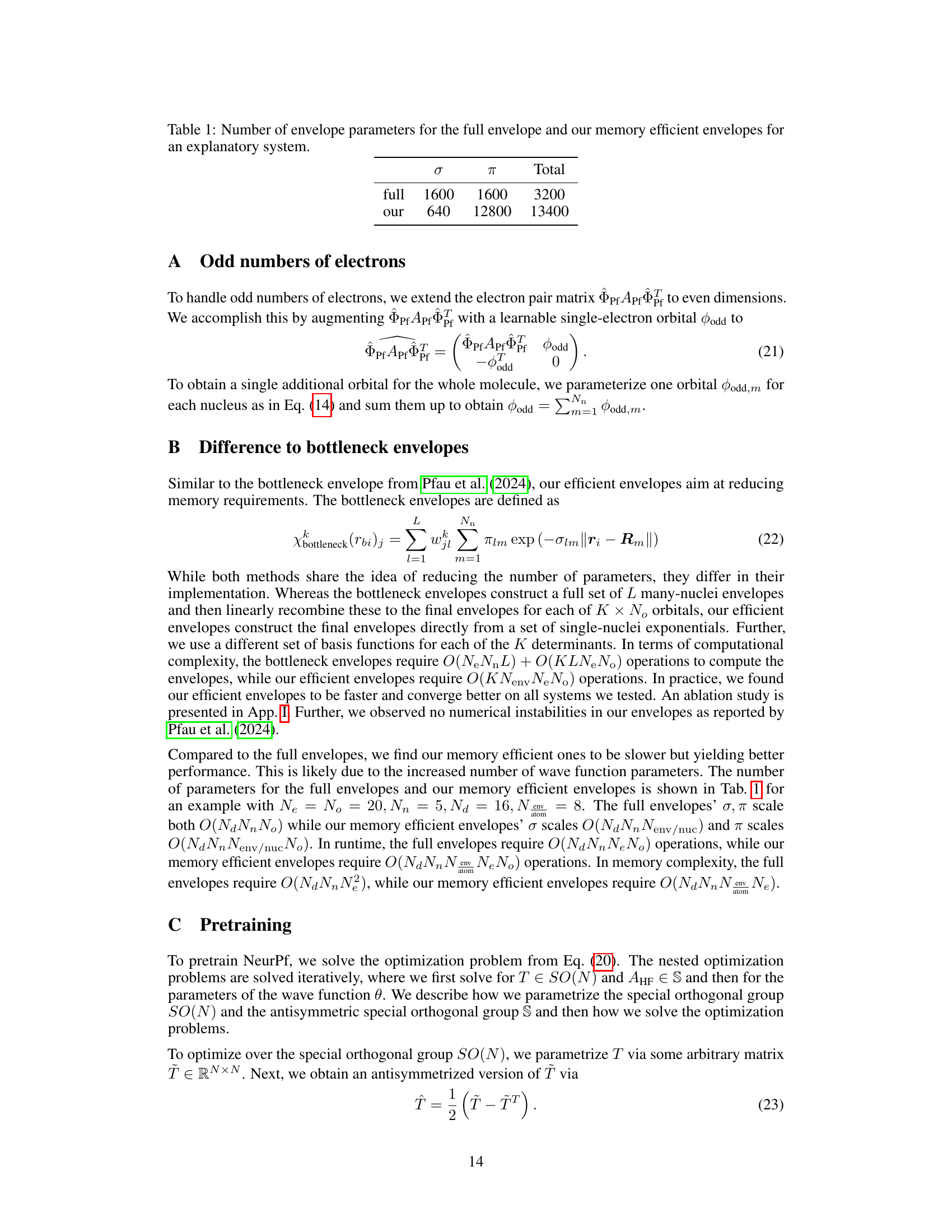
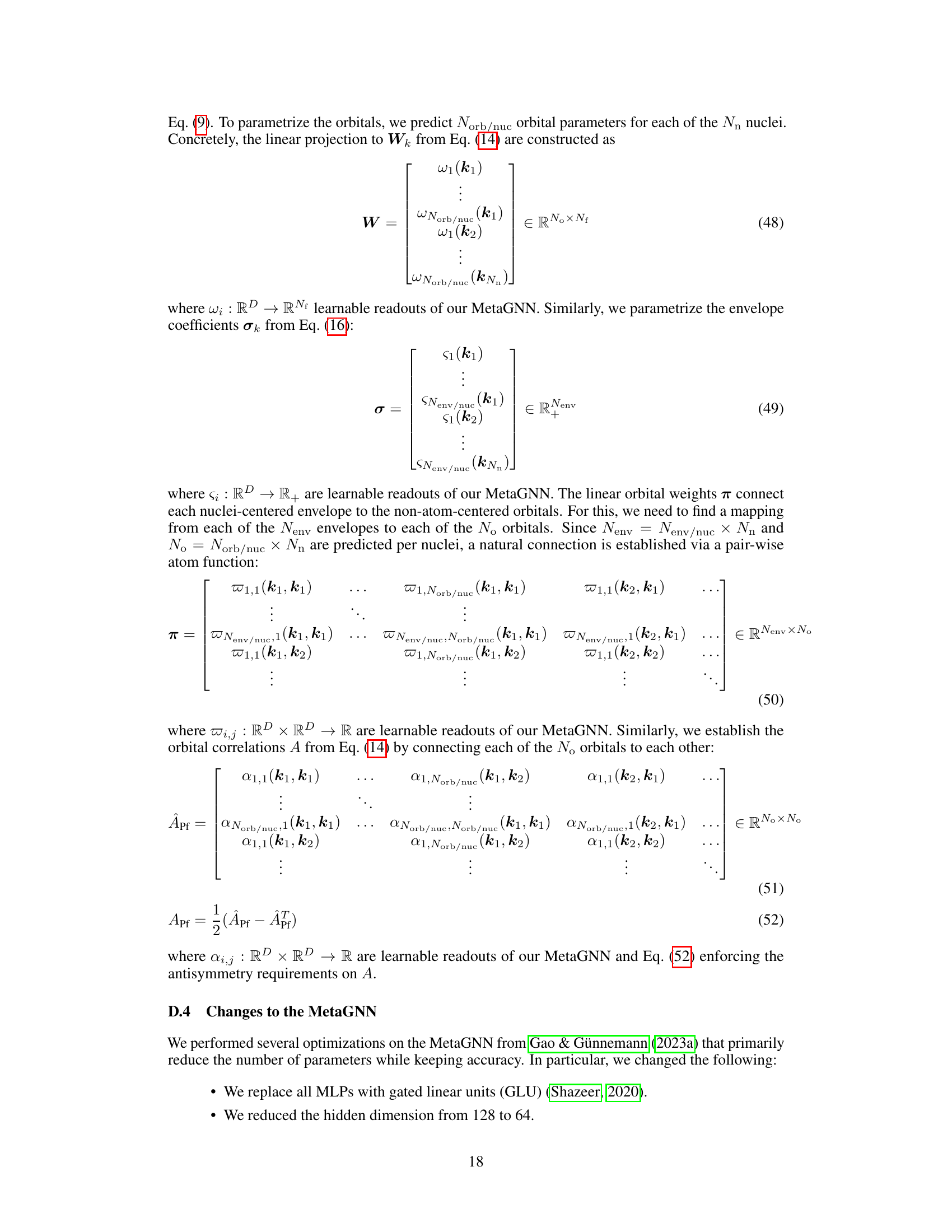
This table compares the number of parameters for two different types of envelopes used in the Neural Pfaffian model: the full envelope and the memory-efficient envelope. The full envelope has a total of 3200 parameters, with 1600 for σ and 1600 for π. The memory-efficient envelope significantly reduces the number of parameters, with a total of 13400 parameters (640 for σ and 12800 for π). This highlights the efficiency gains achieved by using the memory-efficient envelope.
In-depth insights#
Neural Pfaffian#
The heading ‘Neural Pfaffian’ suggests a novel approach to solving the many-electron Schrödinger equation, a computationally expensive problem in quantum chemistry. This approach likely combines the power of neural networks with the mathematical properties of Pfaffians. Neural networks are used to approximate the complex wave functions describing the system’s quantum state, while Pfaffians provide an efficient way to enforce the antisymmetry required by fermionic particles, specifically electrons. This combination offers a potential advantage over traditional methods based on Slater determinants, as Pfaffians can handle systems with an arbitrary number of electrons and spin configurations, leading to improved generalization across different molecules and enhanced accuracy. The ‘Neural’ aspect emphasizes the use of machine learning for approximation, while ‘Pfaffian’ highlights the specific mathematical tool used to guarantee physical correctness. The core innovation likely lies in the seamless integration of these two powerful tools for solving a complex scientific problem. This method potentially provides a more generalizable and efficient solution for various chemical systems, paving the way for further advancements in computational chemistry and related fields.
Pfaffian Wave Function#
The Pfaffian wave function offers a novel approach to representing many-electron systems in quantum chemistry. Unlike the commonly used Slater determinant, which is limited by the requirement of an equal number of orbitals and electrons, the Pfaffian allows for overparametrization, enabling greater flexibility and potentially improved accuracy. This is particularly useful when generalizing across different molecules and structures. The Pfaffian’s inherent antisymmetry property, crucial for satisfying the Pauli exclusion principle, is naturally preserved without the need for discrete orbital selection or constraints. By leveraging the Pfaffian’s mathematical properties, the authors developed a fully learnable neural network wave function. This ‘Neural Pfaffian’ significantly enhances generalization capabilities, surpassing traditional methods by avoiding restrictive constraints and thus obtaining more accurate results. The use of Pfaffians and efficient numerical techniques for calculating Pfaffians becomes crucial for achieving computational efficiency and applicability to larger systems. The combination of Pfaffians and neural networks constitutes a significant advancement in the field of electronic structure calculations, paving the way for more accurate and generalizable models.
Memory Efficiency#
The research paper emphasizes memory efficiency as a crucial aspect of designing neural network wave functions. High-dimensional tensors, inherent in representing many-electron systems, pose significant memory challenges. The authors introduce memory-efficient envelope functions as a solution. These are designed to significantly reduce the number of parameters without compromising accuracy. By using these efficient envelopes, the model can effectively capture the spatial behavior of electrons while keeping the computational cost low. The improved efficiency is achieved through a careful reformulation of the functions, thereby enabling the use of overparameterized wave functions which greatly improves accuracy. This optimization represents a key contribution because it directly addresses one of the biggest challenges in training neural wave functions for large molecular systems, paving the way for more efficient and accurate simulations in computational chemistry.
Generalization#
The concept of generalization is central to the success of the Neural Pfaffian model. The paper highlights the challenges of generalizing neural wave functions across diverse molecules, a problem exacerbated by existing methods’ reliance on hand-crafted, non-learnable algorithms for enforcing electron antisymmetry. The Neural Pfaffian overcomes this limitation by employing Pfaffians instead of Slater determinants, allowing for overparametrization and full learnability. This approach enables the model to generalize effectively across molecules with varying sizes, structures, and electronic configurations, demonstrating significantly improved accuracy and reduced energy errors compared to previous generalized neural wave functions. The success of the model on various datasets, including those with non-equilibrium, ionized, or excited systems, further underscores the power of its generalization capabilities. This is a crucial advancement because it enables the prediction of molecular properties across many different structures, rather than requiring specialized training for each structure, significantly reducing computational cost and broadening applicability.
Future Work#
Future research directions stemming from this Neural Pfaffian work could explore several promising avenues. Extending the model to periodic systems would significantly broaden its applicability, enabling simulations of materials and crystals. Investigating the integration of wave function symmetries could further boost accuracy and generalization capabilities. The computational cost of Pfaffian calculations currently surpasses Slater determinants; therefore, algorithmic optimizations are crucial to enhance efficiency. Exploring the use of different neural network architectures and activation functions could potentially improve performance and stability. Testing NeurPf on larger and more complex molecules beyond the TinyMol dataset would validate its scalability and robustness in diverse chemical environments. Finally, combining NeurPf with other advanced quantum chemistry methods may lead to hybrid approaches capable of achieving even higher accuracy than current gold standards.
More visual insights#
More on figures
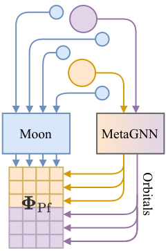
This figure compares the architecture of the Slater determinant and Neural Pfaffian wave functions. The Slater determinant requires exactly N↑ + N↓ orbitals while the Neural Pfaffian uses N° ≥ max{N↑, N↓} orbitals, offering greater flexibility and allowing for overparametrization. The figure highlights the key differences in their structure, emphasizing the advantage of the Neural Pfaffian’s flexibility in handling different numbers of orbitals.
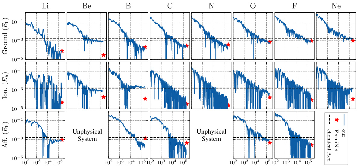
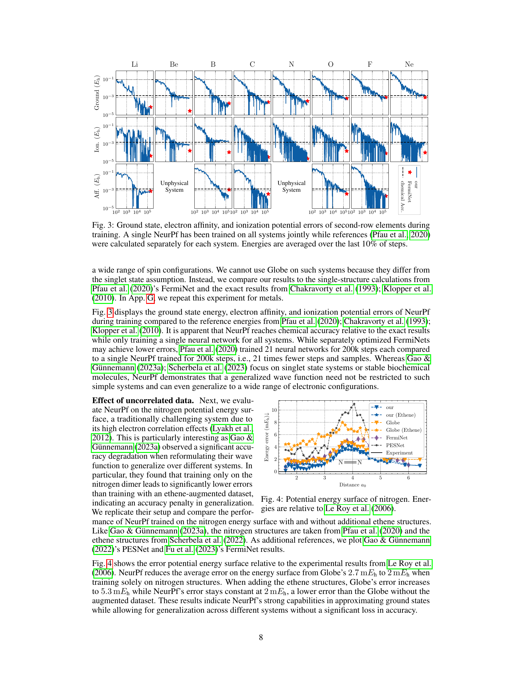
This figure displays the results of training a single Neural Pfaffian (NeurPf) model on second-row elements. The plot shows the errors in ground state energy, electron affinity, and ionization potential during the training process. The key takeaway is that NeurPf achieves chemical accuracy across these properties, even though a single model was trained on all elements simultaneously. This contrasts with previous methods (Pfau et al., 2020) which trained separate models for each element.
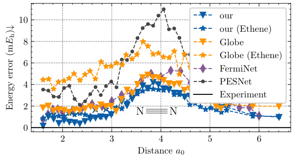
This figure displays the potential energy surface of the nitrogen molecule (N2). It compares the energy errors (in millihartrees, mEh) of different neural network models (NeurPf with and without ethene data augmentation, Globe with and without ethene data, FermiNet, and PESNet) against the experimental data from Le Roy et al. (2006). The x-axis represents the internuclear distance (in units of Bohr radius, a0), and the y-axis represents the energy error. The figure highlights how well the NeurPf model generalizes to different systems even when trained only on the nitrogen dimer, significantly reducing errors compared to other models when incorporating data from additional molecules (ethene) in the training data.
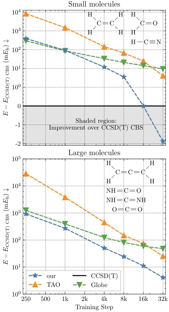
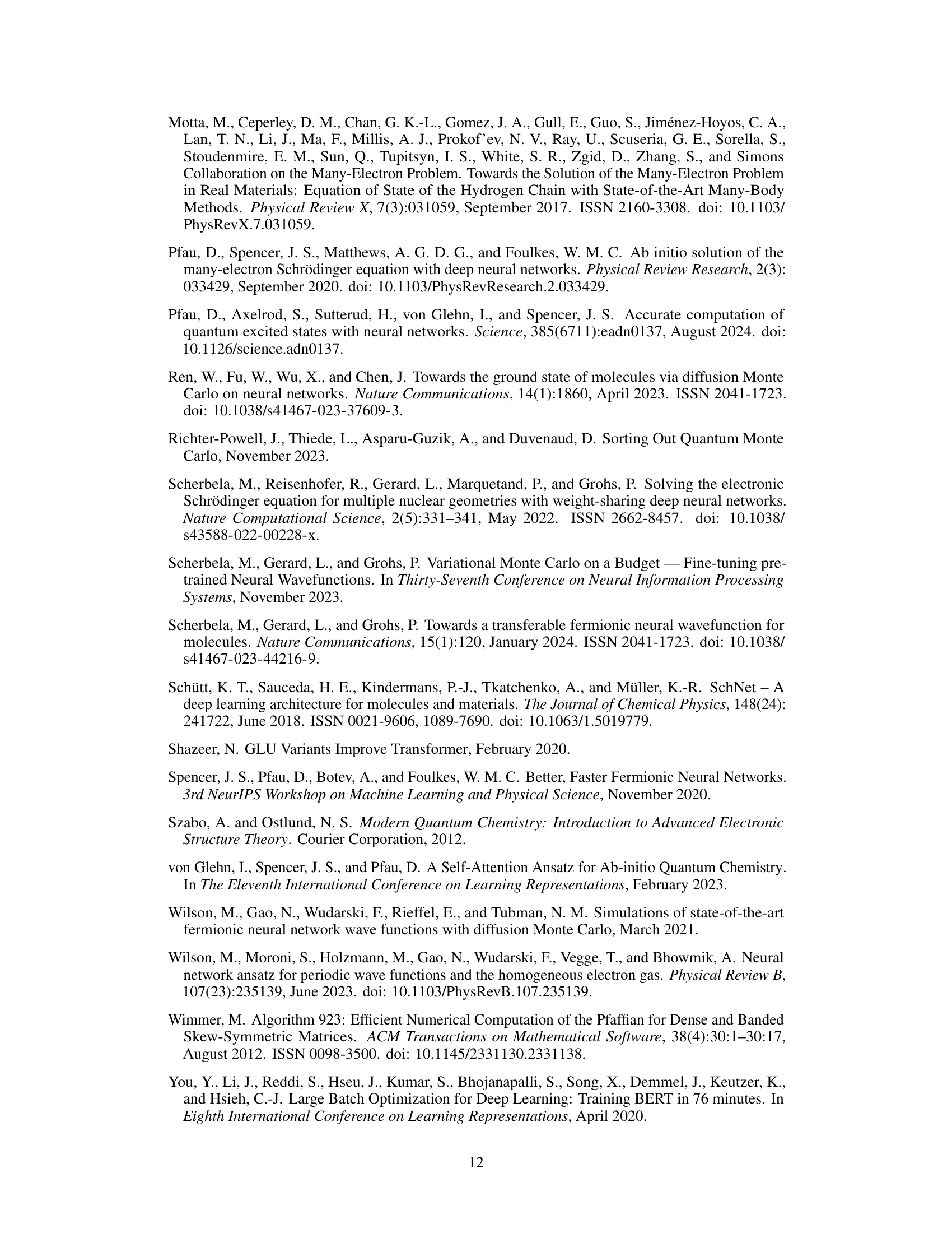
This figure shows the convergence of the mean energy difference on the TinyMol dataset for different models (NeurPf, TAO, Globe) as a function of training steps. The y-axis represents the mean energy difference compared to the CCSD(T) reference energy. The plot is divided into two subplots, one for small molecules and one for large molecules. The shaded region highlights the improvement achieved by NeurPf over the CCSD(T) reference energy. The figure demonstrates that NeurPf converges to lower energy values than the other models and outperforms CCSD(T) for small molecules.
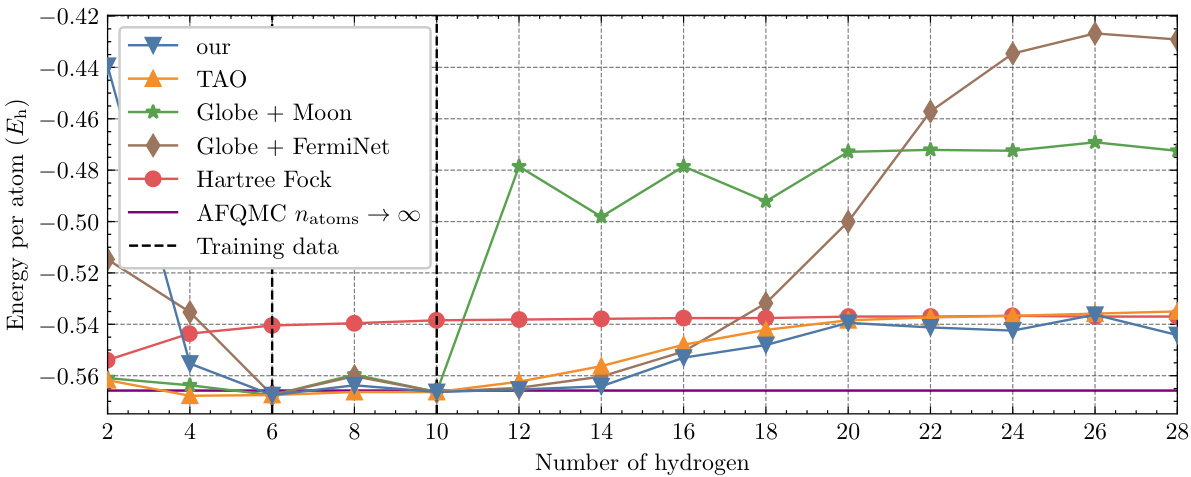
This figure shows the energy per atom of hydrogen chains with varying lengths. A single Neural Pfaffian (NeurPf) model, trained on data from hydrogen chains with 6 and 10 atoms, was used to predict the energy per atom for chains of different lengths. The results are compared against other methods (TAO, Globe + Moon, Globe + FermiNet, Hartree-Fock, and AFQMC), highlighting the NeurPf’s ability to generalize to longer chains not included in its training data.

This figure shows the ionization energy errors for several metal atoms (Na, Mg, Al, K, Ca) during the training of a single Neural Pfaffian (NeurPf) model. The model was trained on both neutral and ionized states of these atoms. The y-axis represents the error in ionization energy, and the x-axis shows the training steps. A horizontal dashed line indicates chemical accuracy. The results demonstrate that NeurPf can accurately predict the ionization energies of these metal atoms, achieving chemical accuracy.
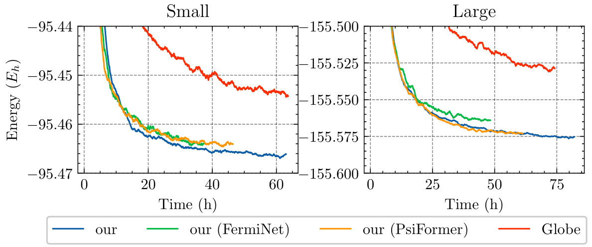
This figure compares the convergence speed of different models on the TinyMol dataset. The left panel shows results for smaller molecules, and the right panel shows results for larger molecules. The x-axis represents training time in hours, and the y-axis represents the total energy. Four different models are compared: NeurPf, NeurPf with FermiNet embedding network, NeurPf with PsiFormer embedding network, and Globe. The results show that NeurPf converges faster and achieves lower energy than the Globe method.
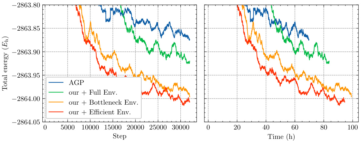
This figure presents an ablation study on the small TinyMol dataset to compare the performance of different envelope functions used within the Neural Pfaffian model. The left graph shows the total energy convergence over training steps, and the right graph shows the convergence over training time. Four model variants are compared: the AGP model, the Neural Pfaffian with full envelopes (from Spencer et al., 2020), the Neural Pfaffian with bottleneck envelopes (from Pfau et al., 2024), and the Neural Pfaffian with the authors’ efficient envelopes. The results illustrate the impact of the different envelope choices on the speed and accuracy of the model’s convergence.
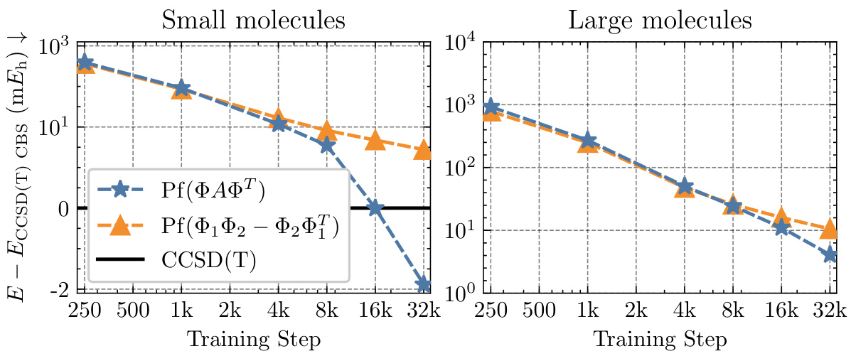
This figure shows the ablation study on the TinyMol dataset with fixed and learnable antisymmetrizers. The results show that using a learnable antisymmetrizer leads to significantly better performance on both the small and large molecules compared to using a fixed antisymmetrizer. The plots show that the mean absolute error decreases significantly faster when using a learnable antisymmetrizer for both small and large datasets, indicating that the model is learning to better approximate the wavefunction.
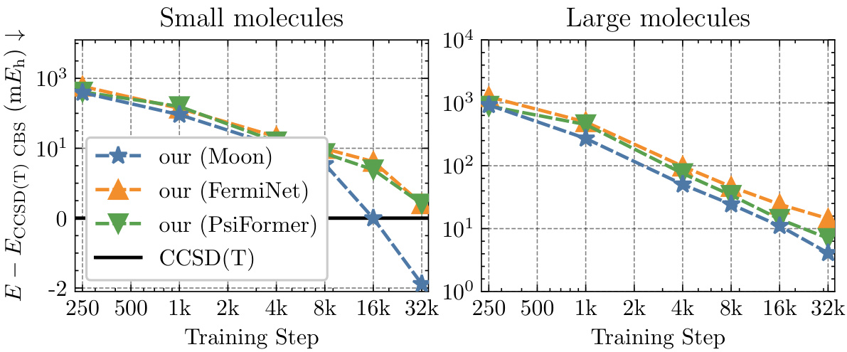
This figure displays the ablation study results on the small TinyMol dataset using different embedding networks. It compares the performance of three different embedding networks: Moon, FermiNet, and PsiFormer, within the Neural Pfaffian framework, and contrasts them against the CCSD(T) reference energies. The plot shows the mean absolute error (MAE) in millihartrees (mEh) against training steps for both small and large molecule sets.
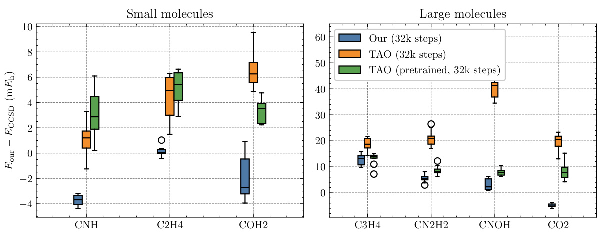
This figure presents box plots comparing the energy per molecule calculated by NeurPf, TAO, and a pretrained version of TAO on the TinyMol dataset. The dataset includes small and large molecule subsets, each containing 10 different molecular structures. The box plots display the median, interquartile range, and 1.5 times the interquartile range of the energy for each molecule, enabling a visual comparison of the performance differences between the methods.
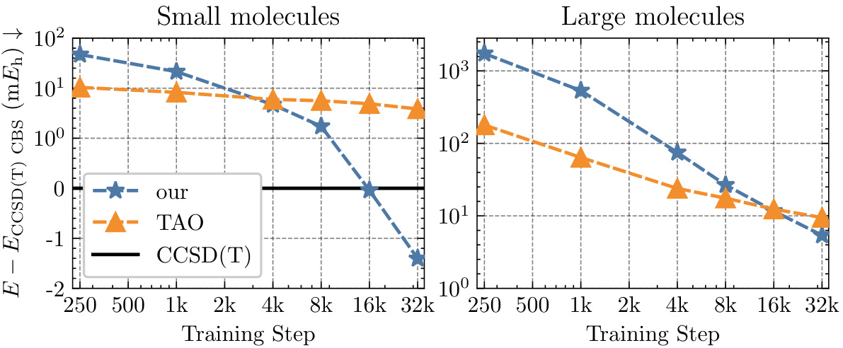
This figure shows the convergence of the mean energy difference between the calculated energies using Neural Pfaffian (NeurPf) and the reference CCSD(T) energies from the TinyMol dataset, as training progresses. The plot includes data for both small and large molecules. The y-axis uses a logarithmic scale for values above 1, and a linear scale for values below 1. The results demonstrate that NeurPf achieves lower energies than the reference CCSD(T) for the small molecules and converges towards more accurate results for the large molecules as training continues. This highlights the efficacy of the Neural Pfaffian approach.
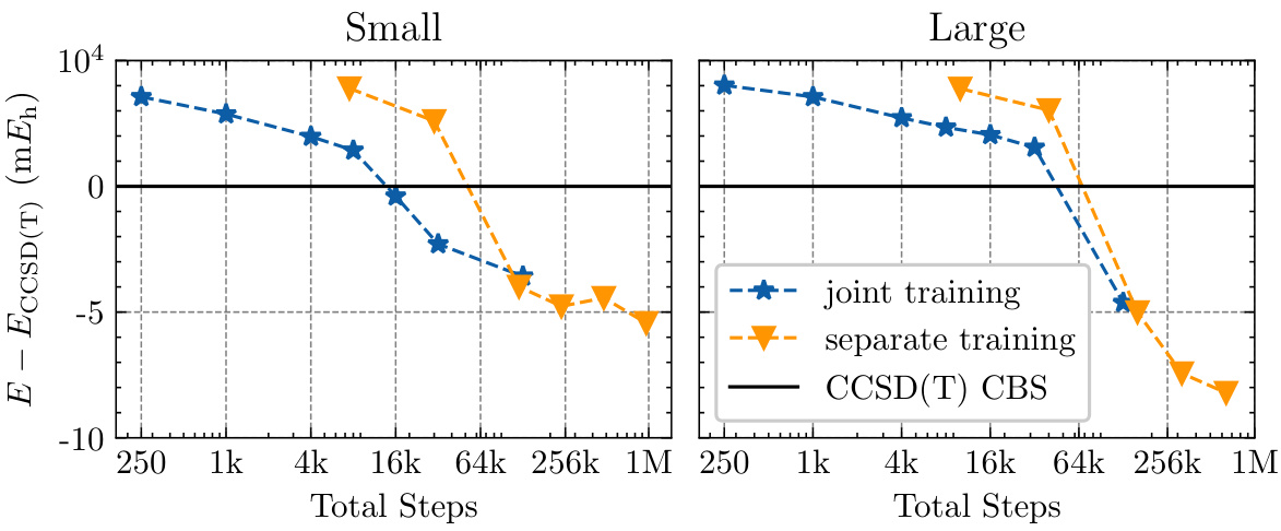
This figure compares the convergence behavior of total energy on the TinyMol dataset using two different training approaches: joint training (a generalized wave function trained on all molecules simultaneously) and separate training (a separate model trained for each molecule). The plot shows the energy error relative to the CCSD(T) CBS reference energy as a function of the total training steps. The results demonstrate the trade-off between training efficiency and accuracy using a generalized model versus a more tailored, but computationally expensive, approach for each molecule.
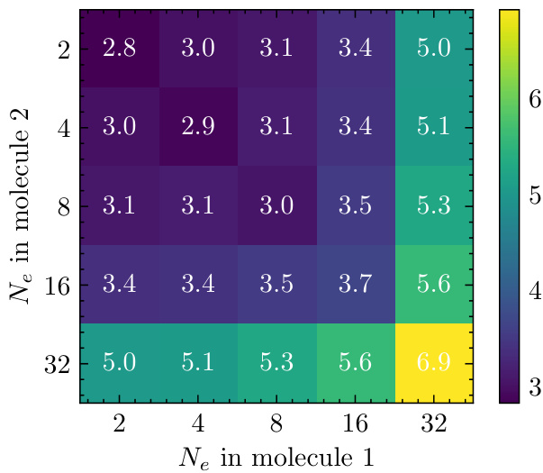
This figure shows a heatmap representing the time taken per training step for various combinations of electron counts in two molecules. The x-axis and y-axis both represent the number of electrons (Ne) in molecule 1 and molecule 2 respectively. Each cell in the heatmap displays the time (in seconds) required per training step for the corresponding combination of electron counts. The color scale indicates the time taken, with darker shades representing shorter times and lighter shades representing longer times. This figure helps in visualizing the impact of the number of electrons on training efficiency. Notably, the diagonal elements (where the number of electrons in both molecules is the same) generally show shorter training times compared to off-diagonal elements, suggesting a potential relationship between computational efficiency and balanced system sizes.
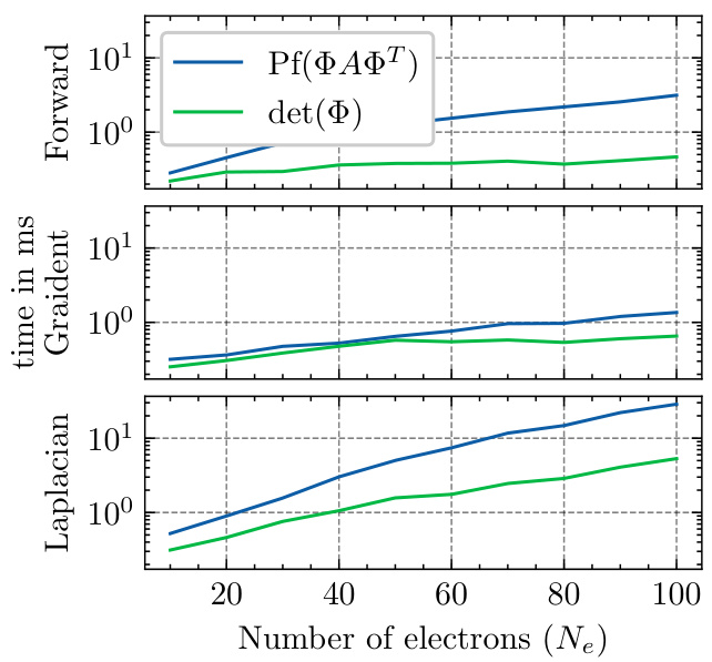
This figure compares the computation time for the forward pass, gradient, and Laplacian of both Slater determinant and Neural Pfaffian wave functions. The x-axis represents the number of electrons (Ne), and the y-axis shows the computation time in milliseconds. It demonstrates that while both have the same complexity O(N³), Neural Pfaffian is approximately 5 times slower than the Slater determinant. This is likely due to the lack of highly optimized CUDA kernels available for the Pfaffian computation.
More on tables
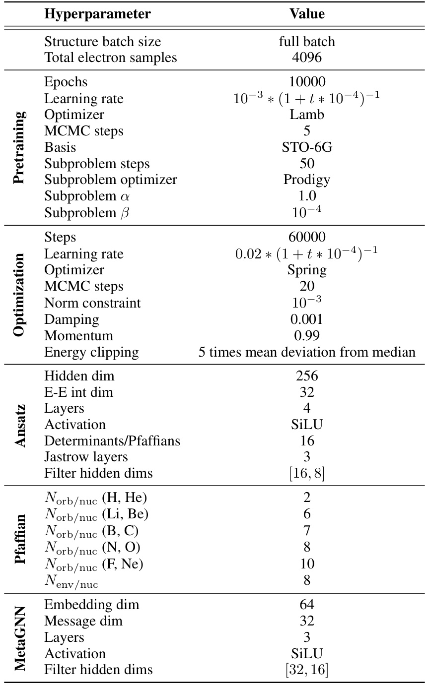
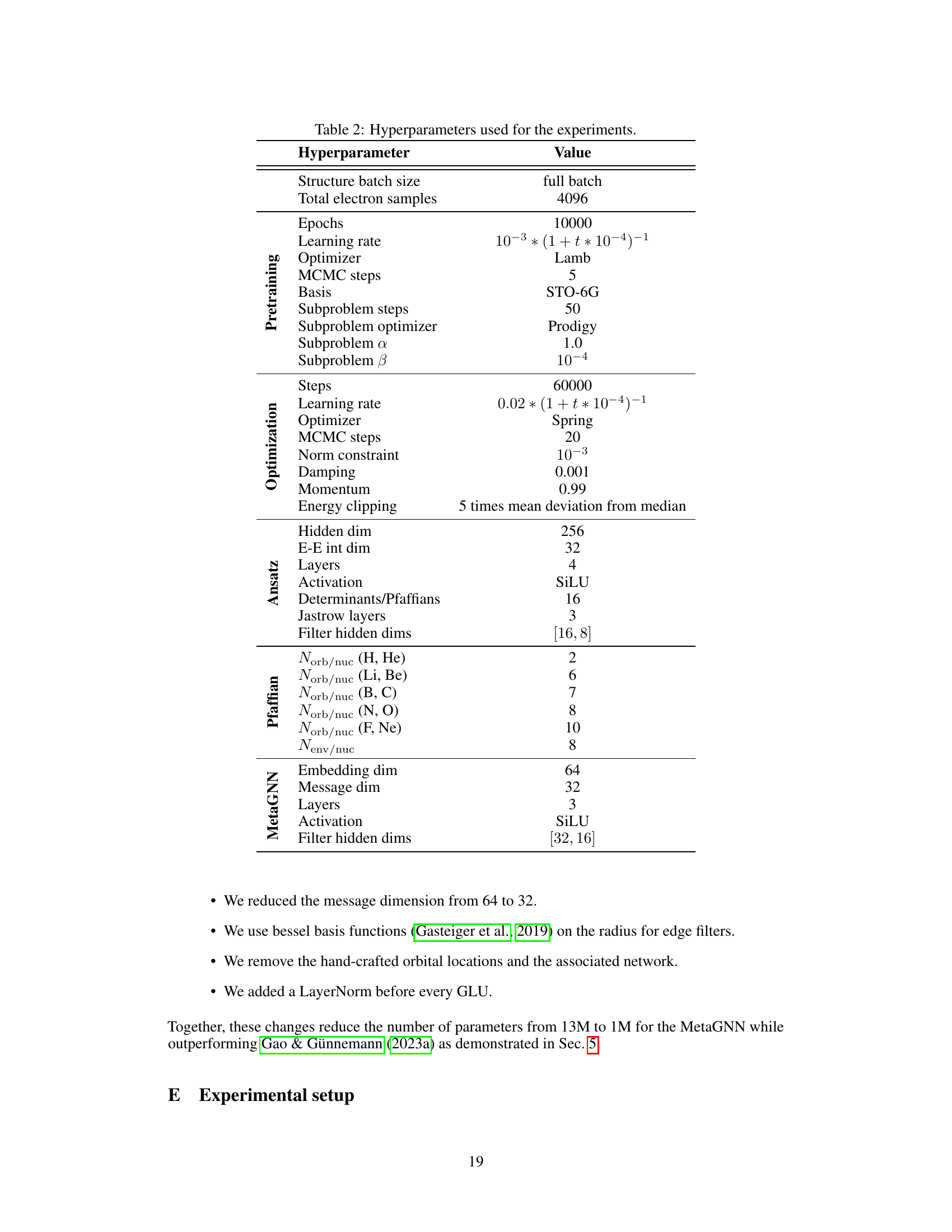
This table lists the hyperparameters used in the experiments described in the paper. It is broken down by category (Pretraining, Optimization, Ansatz, Pfaffian, and MetaGNN) for better readability and provides the value used for each hyperparameter. The hyperparameters relate to various aspects of training the neural network, such as the optimizer used, the learning rate, the number of steps, batch size, activation function and more.
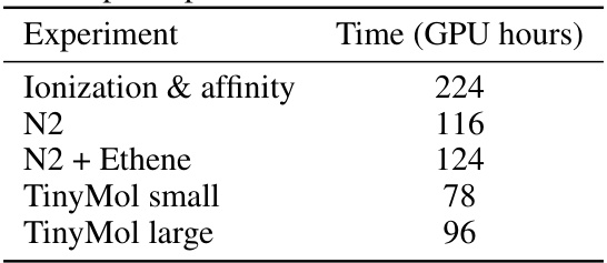
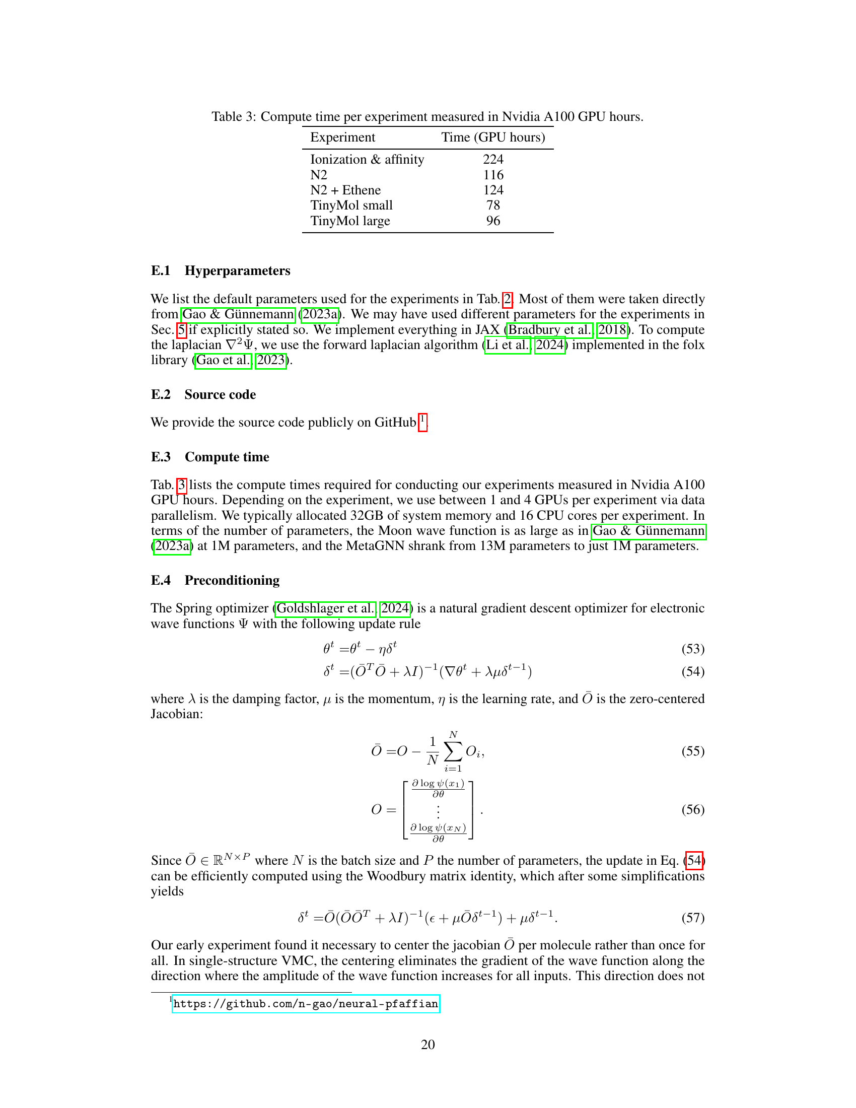
This table presents the computational cost of the experiments performed in the paper, measured in Nvidia A100 GPU hours. The experiments include calculating ionization and electron affinity energies for second-row elements, analyzing the potential energy surface of the nitrogen dimer (with and without additional ethene structures), and evaluating the performance on the TinyMol dataset (small and large subsets). The table provides insights into the computational resource requirements for each task.

This table presents the energy differences (in millihartrees) between the calculated energies using three different methods (Globe, TAO, and the proposed NeurPf method) and the reference CCSD(T) energies for seven small molecules from the TinyMol dataset. The results are shown for two different training step counts (32k and 128k). Negative values indicate that the calculated energy is lower than the reference energy, suggesting higher accuracy.
Full paper#
