↗ OpenReview ↗ NeurIPS Proc. ↗ Hugging Face ↗ Chat
TL;DR#
Existing methods for compressing large language models (LLMs) to 1-2 bits per parameter, while employing fine-tuning, often rely on straight-through estimators (STE) which lack strong theoretical guarantees and can be suboptimal. This research explores and improves quantization-aware fine-tuning strategies, which are crucial given that purely post-training approaches are reaching diminishing returns in accuracy versus bit-width trade-offs.
The paper proposes PV-Tuning, a novel framework that moves beyond STE and provides convergence guarantees in restricted cases. PV-Tuning systematically studies quantization-aware fine-tuning, generalizes and improves upon prior strategies, and achieves the first Pareto-optimal quantization for Llama-2 models at 2 bits per parameter. Experiments demonstrate significant performance improvements over existing methods on various LLM architectures such as Llama and Mistral.
Key Takeaways#
Why does it matter?#
This paper is crucial for researchers in LLM compression and optimization. It introduces PV-Tuning, a novel framework that significantly improves the accuracy of extremely compressed LLMs (1-2 bits/parameter), pushing the boundaries of efficient model deployment. This work addresses limitations of existing fine-tuning techniques, paving the way for more efficient and powerful LLM applications. The Pareto-optimal results for Llama-2 models demonstrate the framework’s practical impact and open new avenues for research in quantization-aware training.
Visual Insights#

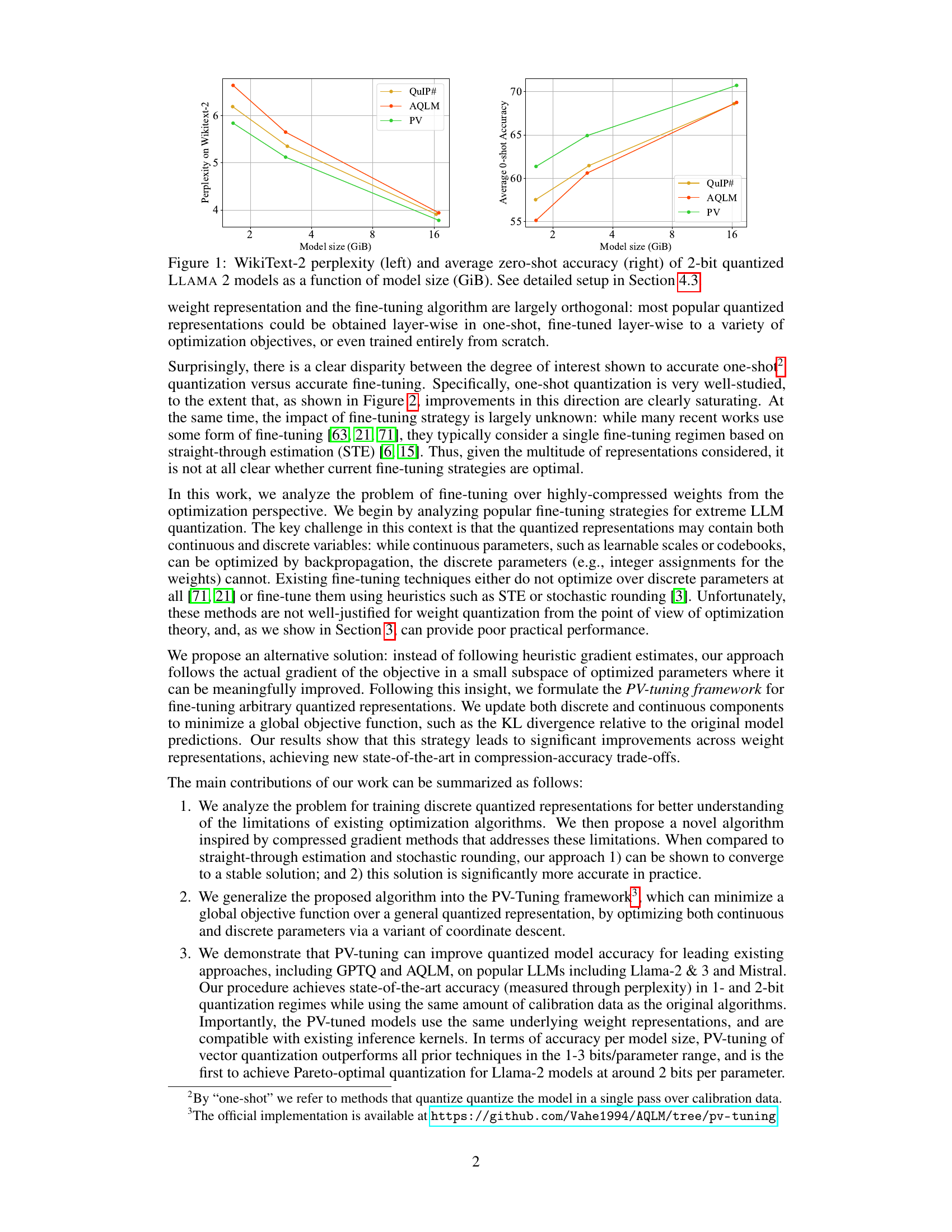
This figure compares the performance of three different 2-bit quantized LLAMA 2 models (QuIP#, AQLM, and PV-Tuning) across various model sizes. The left panel shows the perplexity on the WikiText-2 dataset, a measure of how well the model predicts the next word in a sequence. The right panel shows the average zero-shot accuracy across a set of tasks. Lower perplexity and higher accuracy indicate better performance. The figure demonstrates that PV-Tuning consistently outperforms the other methods across different model sizes.
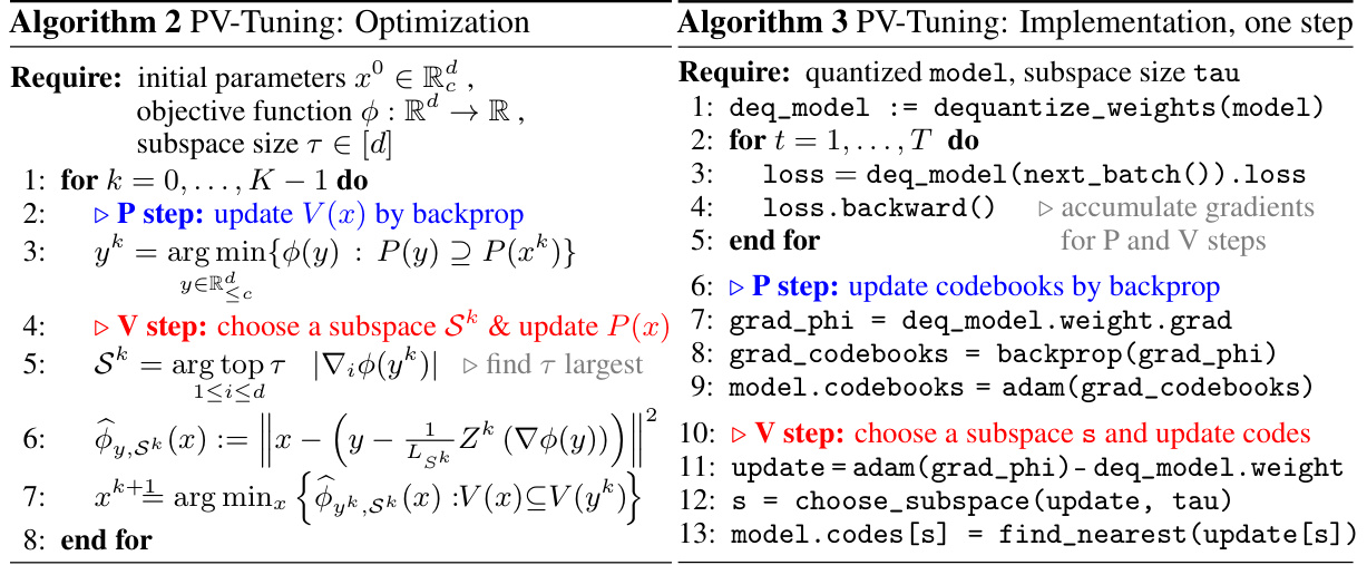
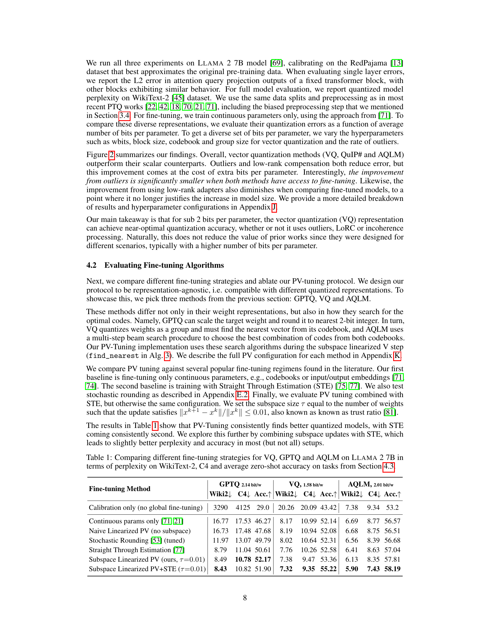
This table compares the performance of different fine-tuning strategies (calibration only, continuous parameters only, naive linearized PV, stochastic rounding, straight-through estimation, subspace linearized PV, and subspace linearized PV + STE) on three different quantized representations (GPTQ, VQ, and AQLM) of the LLAMA 2 7B model. The performance is measured using perplexity on the WikiText-2 and C4 datasets, and average zero-shot accuracy on tasks described in Section 4.3. The table highlights the superior performance of PV-tuning.
In-depth insights#
LLM Extreme Compression#
LLM extreme compression tackles the challenge of significantly reducing the size of large language models (LLMs) while preserving their performance. The primary goal is to make LLMs deployable on resource-constrained devices like mobile phones and edge servers, which typically lack the memory and processing power of cloud-based infrastructure. Approaches involve various quantization techniques, aiming to represent model weights using fewer bits (e.g., 1-2 bits per parameter). This extreme compression necessitates advanced fine-tuning strategies, going beyond simple post-training quantization. Existing methods often rely on straight-through estimators (STE), but these may be suboptimal. Novel approaches like PV-Tuning aim to address these limitations by generalizing and improving fine-tuning strategies, potentially providing convergence guarantees and enhanced performance in extreme compression scenarios. The trade-off between compression level and accuracy remains a critical focus, with research exploring innovative weight representations and optimization techniques to achieve Pareto-optimal results, minimizing the loss in accuracy for a given compression ratio. Ultimately, success in LLM extreme compression promises broader accessibility and affordability of these powerful models.
PV-Tuning Framework#
The PV-Tuning framework introduces a novel approach to fine-tuning quantized large language models (LLMs). It addresses the limitations of existing methods, such as straight-through estimators (STE), which often struggle with extreme compression levels (1-2 bits per parameter). PV-Tuning achieves this by directly optimizing the objective function over both continuous and discrete parameters, avoiding the need for heuristic gradient estimations like STE. The framework uses a coordinate descent strategy that alternates between optimizing continuous parameters (like codebooks) via backpropagation and discrete parameters (like code assignments) through a more principled approach. This enables more accurate updates to the quantized weights, leading to improved performance compared to existing techniques. Its representation-agnostic nature makes it broadly applicable to various quantization methods. The framework provides convergence guarantees in specific cases, further solidifying its theoretical foundation and practical effectiveness.
Quantization Strategies#
This research paper explores various quantization strategies for compressing large language models (LLMs). Post-training quantization (PTQ) methods are analyzed, highlighting their limitations in achieving extreme compression ratios (1-2 bits per parameter). The authors critique the prevalent use of straight-through estimators (STE), arguing it’s suboptimal for extreme compression. Instead, they propose PV-Tuning, a novel framework that goes beyond STE, enabling quantization-aware fine-tuning with convergence guarantees in certain cases. PV-Tuning generalizes existing methods by incorporating a representation-agnostic approach that optimizes both discrete and continuous parameters during fine-tuning. Experimental results on Llama and Mistral models demonstrate that PV-Tuning achieves state-of-the-art results in terms of accuracy-vs-bit-width trade-off. This success is attributed to PV-Tuning’s careful consideration of optimization theory, moving beyond heuristic gradient estimations.
Empirical Results#
An Empirical Results section in a research paper should meticulously document the experimental setup, clearly presenting the methodologies employed and the datasets used. It is crucial to provide comprehensive results, including both quantitative metrics and qualitative observations. The presentation should be structured and easily interpretable, ideally with clear visualization techniques like graphs or tables. The authors must justify the choice of metrics and address the limitations of their experiments, openly acknowledging potential biases. The results should directly support the paper’s claims, with a detailed comparison to relevant baselines or prior works. Furthermore, a discussion of the implications of these findings, alongside any unexpected outcomes, strengthens the study’s impact and invites further investigation. Reproducibility is paramount; therefore, sufficient details on the experimental procedure should be provided to enable independent verification.
Future Research#
The authors suggest several avenues for future work, primarily focusing on improving the PV-Tuning algorithm and extending its application. Improving the subspace selection (Sk) methodology is crucial; while the greedy approach works well, more sophisticated techniques might yield superior results. Applying PV-Tuning to other quantization methods beyond vector quantization, such as those employing low-rank adapters or activation quantization, is a promising area for exploration. Further investigation into alternative loss functions or optimization strategies could also enhance the algorithm’s performance. Finally, they highlight the need for more extensive evaluations, particularly regarding larger LLMs and diverse datasets, to solidify the algorithm’s broader applicability and efficiency. A deeper study into the theoretical properties of the algorithm, especially its convergence behavior under various conditions, would strengthen its foundation. Addressing the increased computational requirements of PV-Tuning compared to simpler fine-tuning strategies is another important area of future work, particularly focusing on developing more efficient implementations suitable for resource-constrained environments.
More visual insights#
More on figures

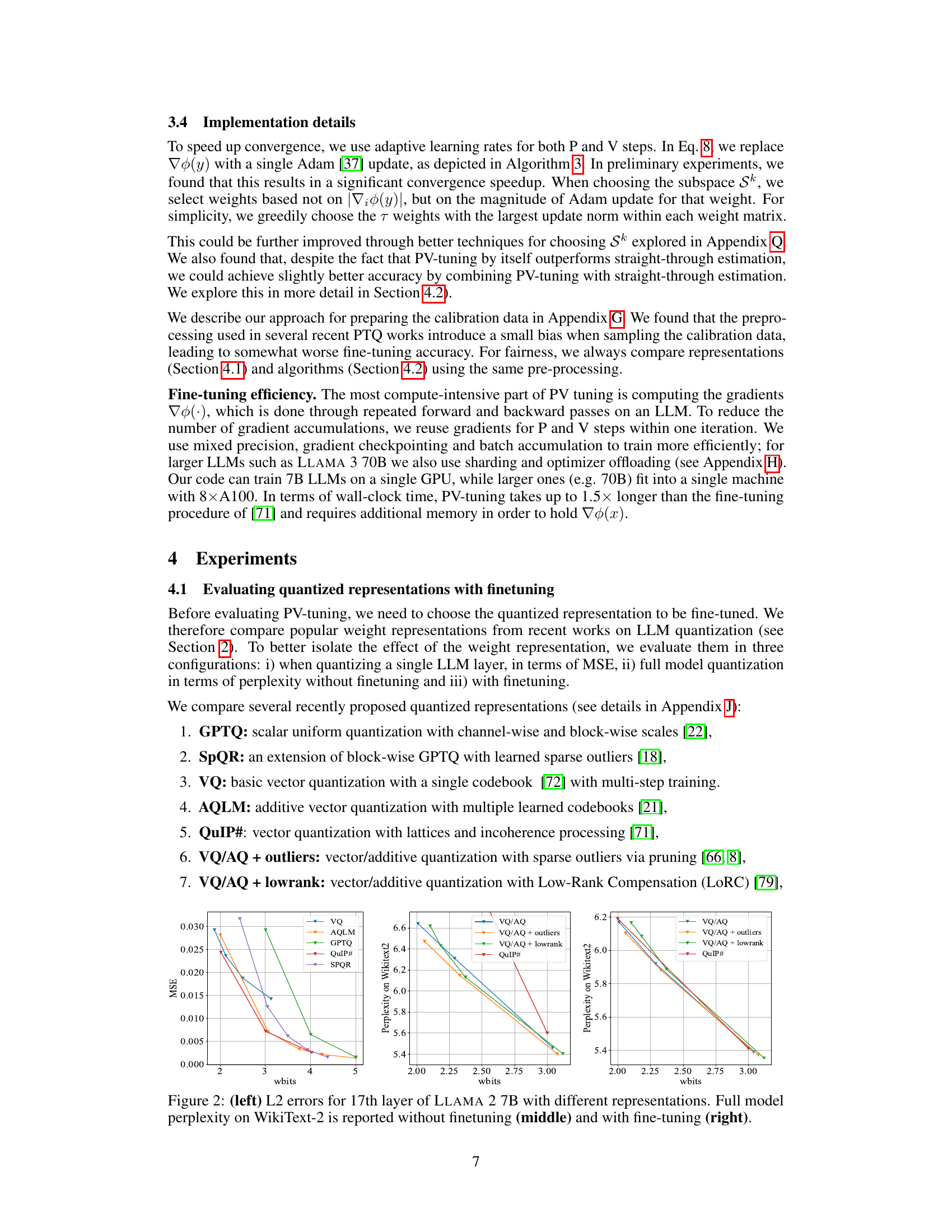
This figure compares several popular weight representations for quantized LLMs. The left panel shows the L2 error for the 17th layer of a Llama 2 7B model after applying different quantization techniques. The middle panel displays the full model’s perplexity on the WikiText-2 benchmark without any further fine-tuning. Finally, the right panel presents the perplexity after applying fine-tuning, demonstrating the impact of fine-tuning on each quantization method. The figure highlights the effectiveness of various representation techniques and the improvement obtained after finetuning.
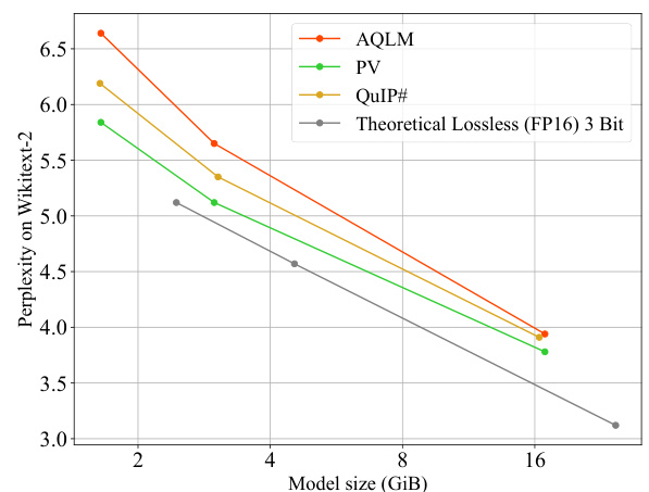
The figure shows the perplexity on the WikiText-2 dataset for 2-bit quantized Llama 2 models with varying sizes. It compares the perplexity of models using different quantization techniques (AQLM, PV-Tuning, QuIP#) against a theoretical lossless baseline (using 3 bits and FP16 precision). The plot demonstrates how perplexity changes with model size and quantization method.

This figure compares different quantization methods in terms of their accuracy-size trade-off. The leftmost plot shows the L2 error for a single layer of a Llama 2 7B model with various quantization techniques. The middle plot presents the perplexity on WikiText-2 for the full models without fine-tuning, and the rightmost plot depicts the same for models after fine-tuning. The figure highlights the performance gains achieved through PV-Tuning, especially in the low-bit regime.

This figure shows the learning curves of PV-Tuning (subspace 0.01) and Straight-Through Estimation (STE) when fine-tuning a TinyLlama model. The model uses 2x8g8 AQLM quantization, meaning it has 2 codebooks with 8 bits each, and the input groups are of size 8. The y-axis represents the perplexity on the WikiText2 dataset, and the x-axis represents the training step. The shaded areas represent the standard deviation across multiple runs. The plot illustrates the convergence behavior of both methods and the relative performance in terms of perplexity.
This figure compares three different methods (QuIP#, AQLM, and PV-Tuning) for 2-bit quantization of LLAMA 2 models of varying sizes, evaluating their performance on the WikiText-2 perplexity benchmark and average zero-shot accuracy. It visually demonstrates the relative performance gains of PV-Tuning over existing methods in terms of both perplexity (lower is better) and zero-shot accuracy (higher is better) as the model size increases. Detailed experimental setup is described in Section 4.3 of the paper.
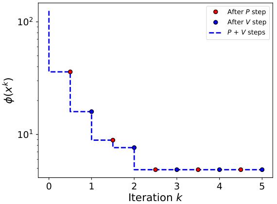
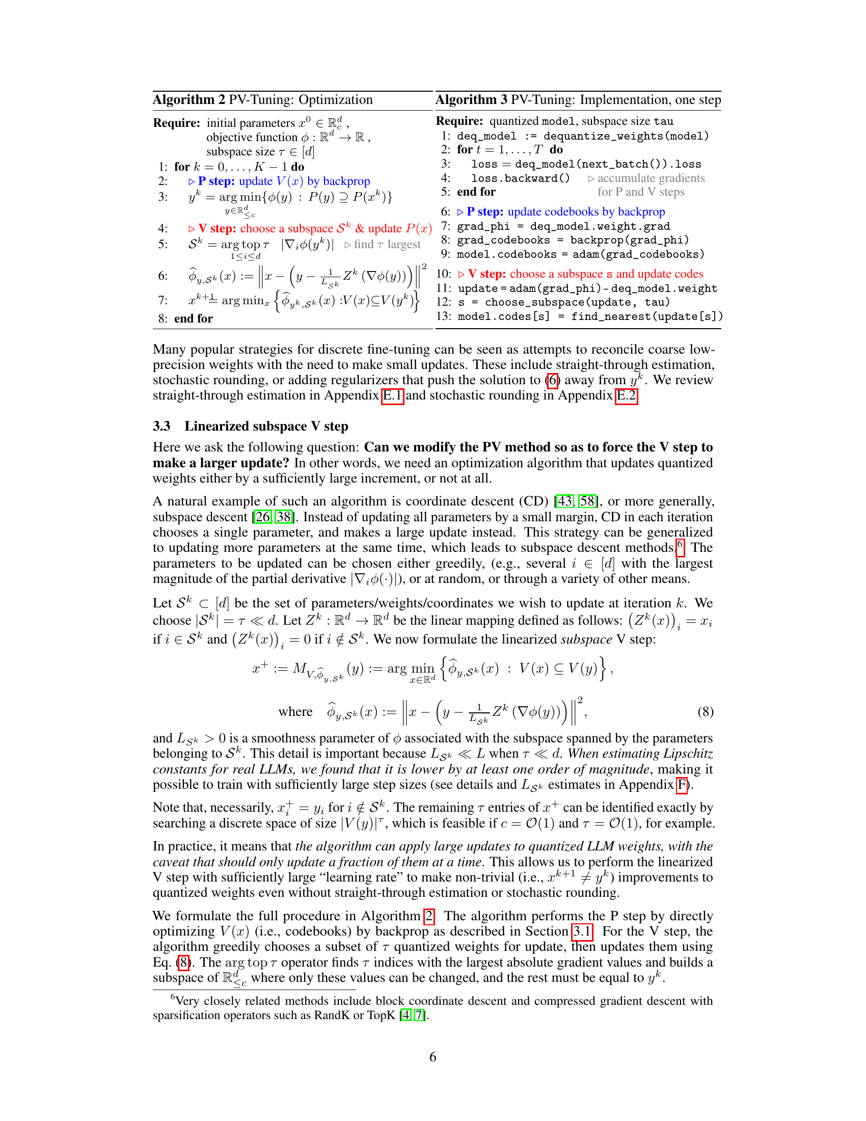
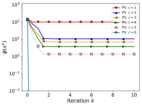
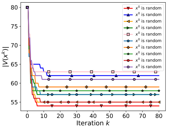
This figure shows the results of applying the PV algorithm to a small-scale problem with a 6-dimensional quadratic objective function. The algorithm’s performance is evaluated for different numbers of unique values (c) in the weight vectors. The starting point for each run is randomly chosen using Algorithm 6, ensuring variation in initial conditions. Subplots illustrate the algorithm’s convergence for various values of c and the effect of separate P and V steps on loss function.

This figure shows the performance of 2-bit quantized Llama 2 models on two tasks: WikiText-2 perplexity and average zero-shot accuracy. The x-axis represents the model size in GiBs, demonstrating how performance changes with varying model sizes after 2-bit quantization. The results compare three different methods: QuIP#, AQLM, and PV-Tuning.
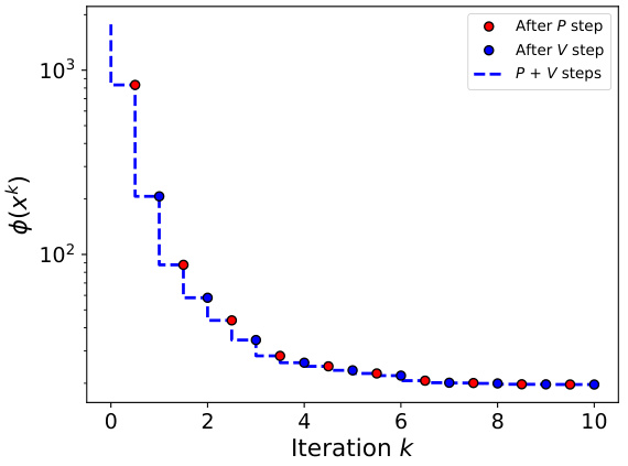
This figure shows the results of applying the PV algorithm to a small-scale problem (d=6, c=[1,6]) with a quadratic objective function. The algorithm is run multiple times (r=50) with different random starting points to show its behavior and convergence properties. The subplots demonstrate: (a) convergence curves for different values of ‘c’, representing varying levels of compression; (b) the effect of P and V steps on the objective function for c=3. The results highlight the algorithm’s convergence and the iterative nature of P and V steps, showing that both are needed to find an accurate solution. The scale in (a) is logarithmic, explaining why the line for c=6 is not visible, as it is very close to the minimum loss (0).

This figure shows the results of experiments using the Linearized PV algorithm with different numbers of iterations (T) for the linearized V-step. Subfigure (a) compares the convergence rates of the Linearized PV algorithm with different values of T, showing that increasing T leads to faster convergence but similar final accuracy. Subfigure (b) illustrates the influence of P and V steps on the loss function for a specific value of T (T=2), demonstrating the iterative improvement achieved by alternating between these steps.
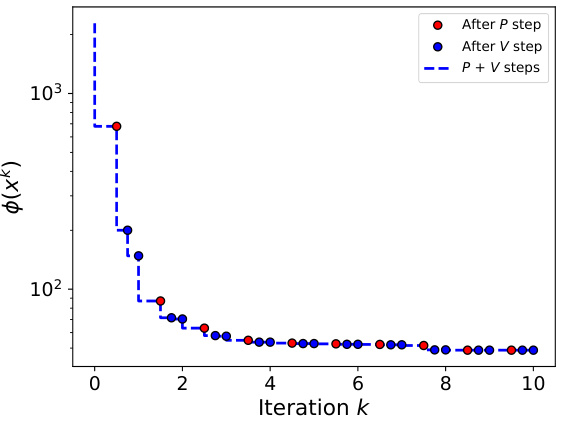
This figure shows the results of applying the PV algorithm to a small-scale problem with a quadratic objective function. The dimensionality (d) is 6, and the maximum number of unique values (c) is varied from 1 to 6. The algorithm is run 50 times with different randomly chosen starting points to demonstrate its behavior. The subplots illustrate the convergence of the algorithm for different values of c and show the impact of the P and V steps on the loss function.

This figure compares three different algorithms for optimizing a quantized model: the exact PV algorithm, the linearized PV algorithm, and the linearized PV algorithm with sparse updates. The x-axis represents the iteration number, and the y-axis shows the objective function value (loss). The results demonstrate that the linearized PV algorithm converges to a lower accuracy compared to the exact PV algorithm. However, incorporating sparse updates into the linearized PV algorithm leads to a significant improvement in accuracy, converging to a value close to that of the exact PV algorithm. There is also a trade-off; the convergence speed is slower with sparse updates compared to the linearized PV algorithm alone.
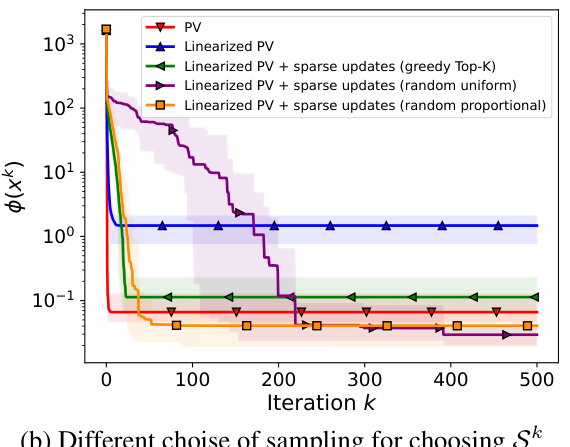
This figure compares three different algorithms in terms of their convergence behavior and final accuracy. The algorithms are: the exact PV algorithm, the linearized PV algorithm, and the linearized PV algorithm with sparse updates. The results show that the exact PV algorithm converges to the best accuracy, while the linearized PV algorithm converges to a worse accuracy. The linearized PV algorithm with sparse updates converges to an accuracy that is in between the other two algorithms.
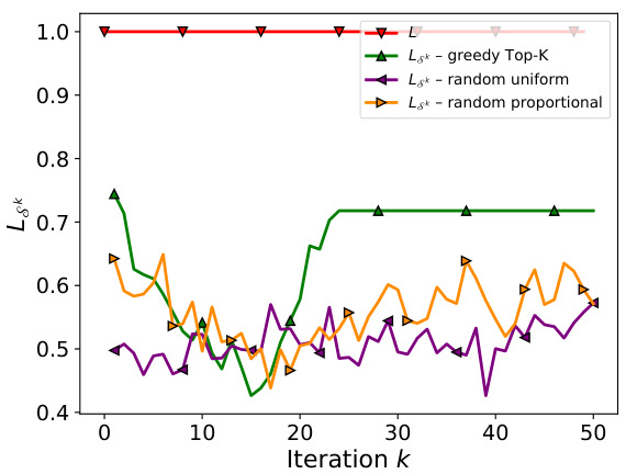
This figure compares the performance of three PV algorithms: the exact PV algorithm, the linearized PV algorithm, and the linearized PV algorithm with sparse updates. The x-axis represents the iteration number, and the y-axis represents the value of LSkk (a measure of the smoothness of the objective function in the sparse subspace). The figure shows that the exact PV algorithm converges to the best accuracy, but the linearized PV algorithm with sparse updates converges to a better accuracy than the linearized PV algorithm alone, although it takes more iterations to converge. Different methods for selecting the sparse subspace (greedy Top-K, random uniform, and random proportional) are also shown, demonstrating that the greedy Top-K method generally yields the fastest convergence.
This figure compares the performance of three different 2-bit quantized LLAMA 2 models (QuIP#, AQLM, and PV-Tuning) across various model sizes. The left panel shows the perplexity on the WikiText-2 benchmark, a measure of how well the model predicts the next word in a sequence. The right panel displays the average zero-shot accuracy across a range of tasks. The results indicate that PV-Tuning consistently outperforms QuIP# and AQLM in terms of both perplexity and zero-shot accuracy, particularly as the model size increases.
More on tables

This table compares the performance of different fine-tuning strategies (Calibration only, Continuous params only, Naive Linearized PV, Stochastic Rounding, Straight Through Estimation, Subspace Linearized PV, Subspace Linearized PV+STE) on three different quantized representations (VQ, GPTQ, AQLM) of the LLAMA 2 7B model. The performance is measured using perplexity on WikiText-2 and C4 datasets, as well as average zero-shot accuracy across multiple tasks (as defined in Section 4.3). The table highlights the relative improvements achieved by each fine-tuning method compared to others.
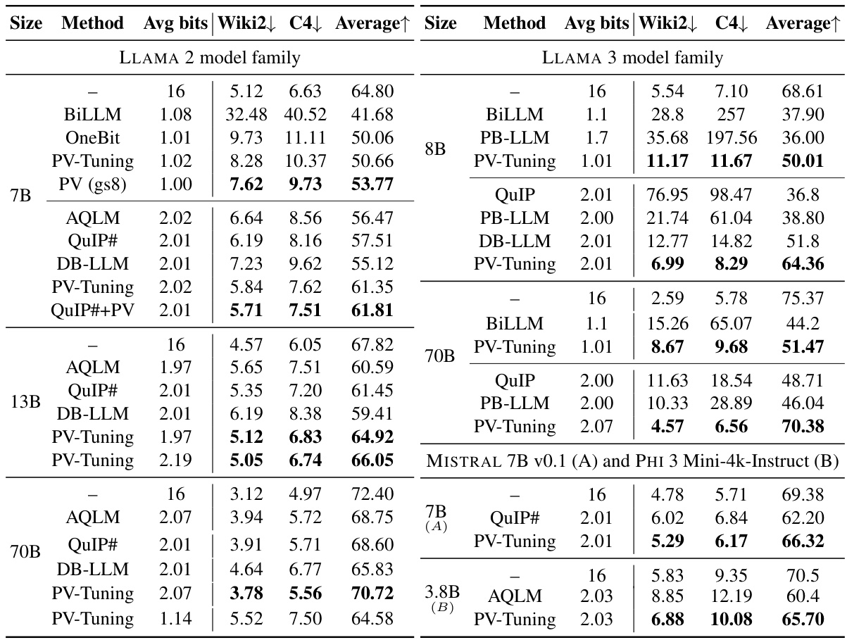
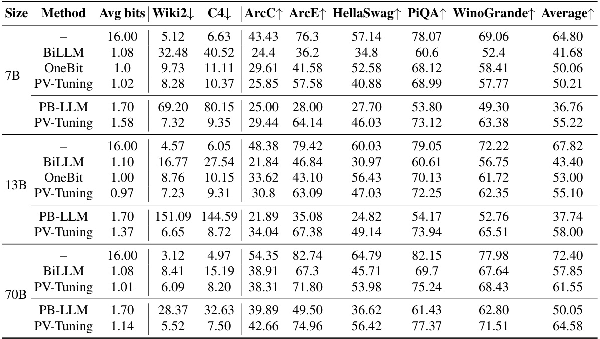
This table presents a comparison of various large language models (LLMs) after quantization using different methods. It shows the perplexity scores on the WikiText-2 and C4 datasets, along with the average zero-shot accuracy across five tasks. The models are grouped by size (7B, 13B, 70B), and the results are shown for different average bits per parameter, demonstrating the trade-off between model size and accuracy after quantization.

This table compares the performance of three different fine-tuning strategies (continuous parameters only, straight-through estimation, and stochastic rounding) across three different quantized representations (VQ, GPTQ, and AQLM) of the Llama 2 7B model. The performance is measured using perplexity on the WikiText-2 and C4 datasets, as well as average zero-shot accuracy across several tasks described in section 4.3 of the paper. The table aims to show the effectiveness of each fine-tuning approach on achieving a balance between accuracy and compression.
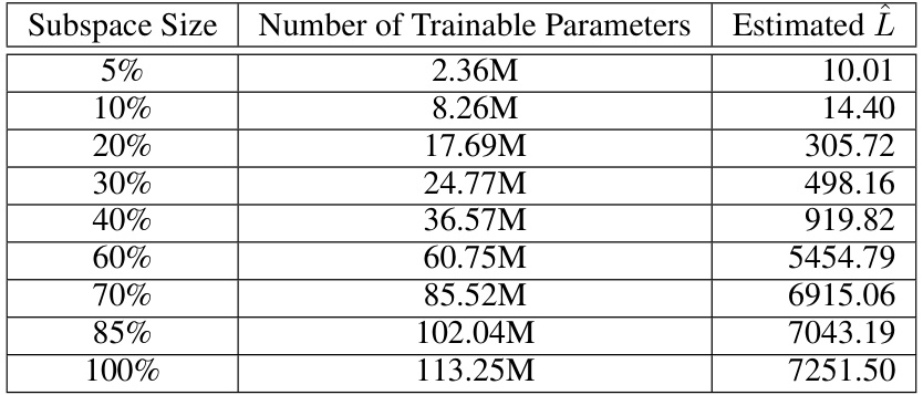
This table presents the estimated L-smoothness constant (L) for the Llama-160m model along the gradient descent (GD) trajectory using Schema I. Different subspace sizes (5%, 10%, 20%, 30%, 40%, 60%, 70%, 85%, 100%) are considered, showing the number of trainable parameters for each subspace and the corresponding estimated L value. The table illustrates the non-increasing property of the L-smooth constant when restricting the subspace of training variables, demonstrating a significant decrease in L as the subspace size reduces.
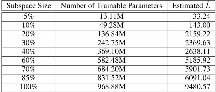
This table presents the estimated L-smoothness constant (L) for the TinyLlama-1.1B language model using two different schemas. The L-smoothness constant is a measure of how curved the objective function is. Lower values indicate a smoother, more easily optimized function. The table shows how L changes as the size of the subspace used for gradient descent is varied. The subspace size is represented as a percentage (5%, 10%, etc.), indicating the proportion of trainable parameters updated in each iteration of the optimization process. The ‘Number of Trainable Parameters’ column shows the number of parameters being optimized within the specified subspace. The ‘Estimated L’ column shows the estimated L-smoothness constant for that subspace size, obtained through gradient descent. Schema I refers to a specific method for estimating L that does not fully capture local curvature of the objective function.

This table presents the estimated L-smoothness constant (L) along the gradient descent (GD) trajectory for the LLama-160m model using Schema I. The L-smoothness constant is calculated for different subspace sizes (5%, 10%, 20%, 30%, 40%, 60%, 70%, 85%, and 100%), which represents the percentage of trainable parameters considered. The table shows the number of trainable parameters within each subspace and the corresponding estimated L value. Schema I is an estimation method that doesn’t capture local curvature, providing an upper bound estimate of the true L-smoothness constant along the GD trajectory.

This table presents the estimated L-smoothness constant ((\hat{L})) for the TinyLlama-1.1B language model using two different schemas (Schema I and II) along the gradient descent (GD) trajectory. The table shows how the estimated (\hat{L}) changes as the size of the subspace used in GD varies from 5% to 100% of the total trainable parameters. Schema I estimates (\hat{L}) without considering local curvature, while Schema II captures local curvature by utilizing an approximate hessian-vector product.

This table compares the WikiText-2 perplexity of different quantization methods applied to the Llama 2 7B model, both with and without fine-tuning. It shows the average bits per weight used by each method and the resulting perplexity scores before and after fine-tuning. The setup for each method is consistent with Section 4.1 of the paper. The table allows for a comparison of the effectiveness of various quantization techniques and the impact of fine-tuning on model performance.

This table compares the performance of different fine-tuning strategies (calibration only, continuous parameters only, naive linearized PV, stochastic rounding, straight-through estimation, subspace linearized PV, and subspace linearized PV+STE) on three different quantized representations (GPTQ, VQ, and AQLM) of the LLAMA 2 7B model. The evaluation metrics include perplexity on WikiText-2 and C4 datasets, and average zero-shot accuracy across multiple downstream tasks. The table highlights the superior performance of subspace linearized PV and its combination with STE across various representations, showcasing its robustness and effectiveness.

This table presents a comparison of different fine-tuning strategies applied to the Llama-2 7B model quantized using the QuIP# algorithm. It shows the performance in terms of perplexity (WikiText-2 and C4 datasets) and average zero-shot accuracy across five tasks. The comparison includes QuIP# without fine-tuning, QuIP# with the built-in fine-tuning method, an improved version of the built-in fine-tuning, and finally QuIP# combined with PV-Tuning. The primary metrics considered are WikiText-2 perplexity, C4 perplexity, and average zero-shot accuracy.

This table presents the results of experiments conducted to evaluate the impact of varying group size and codebook size on the performance of the Vector Quantization with PV-Tuning method. It shows the WikiText-2 and C4 perplexity scores, as well as the average zero-shot accuracy across five different tasks, for various combinations of group size and codebook size. The goal is to determine the optimal settings that balance model size and performance.
This table compares different fine-tuning strategies (Calibration only, Continuous params only, Naive Linearized PV, Stochastic Rounding, Straight Through Estimation, Subspace Linearized PV, and Subspace Linearized PV+STE) across three different quantized weight representations (GPTQ, VQ, and AQLM) on the Llama 2 7B model. The performance metrics include perplexity on the WikiText-2 and C4 datasets and average zero-shot accuracy across several tasks. The table helps to analyze the effectiveness of different fine-tuning algorithms and highlight the superior performance of PV-Tuning in achieving optimal compression-accuracy trade-offs.
This table presents a comparison of various large language models (LLMs) compressed to different bitwidths using different quantization methods. It shows the perplexity scores on the WikiText-2 and C4 datasets, as well as the average accuracy across five zero-shot tasks. The models include Llama 2 and 3, Mistral, and Phi-3 Mini-4k-Instruct. The table helps to understand the trade-off between model size (bits per parameter) and performance across different models and quantization techniques. Lower perplexity and higher accuracy are better.

This table presents a large-scale evaluation of the PV-Tuning algorithm across different large language models (LLMs) and bitwidths. It compares the performance of PV-Tuning against existing quantization methods (QuIP, BiLLM, PB-LLM, DB-LLM, AQLM, OneBit, and QuIP#) in terms of perplexity on the WikiText-2 and C4 benchmark datasets, as well as average zero-shot accuracy across five different tasks (WinoGrande, PiQA, HellaSwag, ARC-easy, and ARC-challenge). The table shows the model size, the quantization method used, the average number of bits per weight parameter, and the resulting perplexity and accuracy scores. The arrows indicate whether a higher or lower value is better for each metric. The results demonstrate that PV-Tuning achieves state-of-the-art performance across various models and bitwidths.

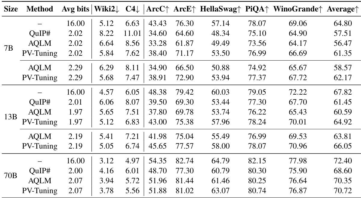
This table presents the results of quantizing Llama 2 models to 2-2.3 bits per weight using different methods. It shows the perplexity scores on WikiText-2 and C4 datasets and the average accuracy across five zero-shot tasks for each method and bit-width. The table allows comparison of different quantization methods in terms of their accuracy-compression trade-off.

This table presents a comparison of different LLM quantization methods across various model sizes and bit-widths. The metrics used for comparison are perplexity scores on the WikiText-2 and C4 datasets, along with average accuracy across five zero-shot tasks (WinoGrande, PiQA, HellaSwag, ARC-easy, ARC-challenge). Lower perplexity and higher accuracy are preferred. The table helps to assess the trade-off between model size, bit-width (bits per parameter), and the performance achieved by each method. It showcases the performance of PV-Tuning in comparison to several state-of-the-art quantization techniques, demonstrating its superior performance particularly at low bit-widths (1-2 bits/parameter).

This table compares the performance of three different fine-tuning strategies (continuous parameters only, straight-through estimation, and stochastic rounding) across three different quantized representations (VQ, GPTQ, and AQLM) for a Llama 2 7B model. The results are measured in terms of perplexity on the WikiText-2 and C4 datasets and average zero-shot accuracy across a set of tasks. This table helps to assess the effectiveness of various fine-tuning approaches in improving the accuracy of quantized LLMs.
Full paper#
