↗ OpenReview ↗ NeurIPS Proc. ↗ Hugging Face ↗ Chat
TL;DR#
Many machine learning optimization techniques depend on learning rate schedules. However, these schedules necessitate determining the training duration beforehand, which limits their applicability. Moreover, the theoretical guarantees often don’t translate to real-world performance, creating a theory-practice gap. This paper focuses on addressing these shortcomings.
This research introduces ‘Schedule-Free’ optimization, a novel approach that completely forgoes learning rate schedules while maintaining state-of-the-art performance across various tasks. The core contribution is a unified theoretical framework linking iterate averaging and learning rate schedules, leading to a new momentum-based algorithm. This approach matches and often surpasses schedule-based approaches in practice, demonstrating significant improvement in efficiency and usability.
Key Takeaways#
Why does it matter?#
This paper is crucial because it addresses a significant gap between optimization theory and practical applications in machine learning. Current methods rely on learning rate schedules requiring prior knowledge of the training duration. The Schedule-Free approach eliminates this need, achieving state-of-the-art performance across diverse problems. This offers researchers a more efficient, theoretically sound method, and opens new avenues in large-scale optimization.
Visual Insights#

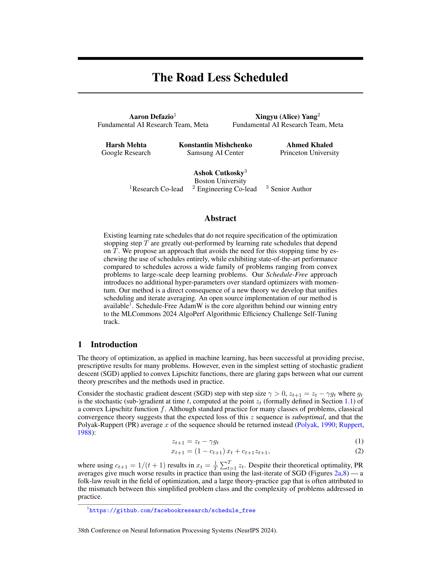
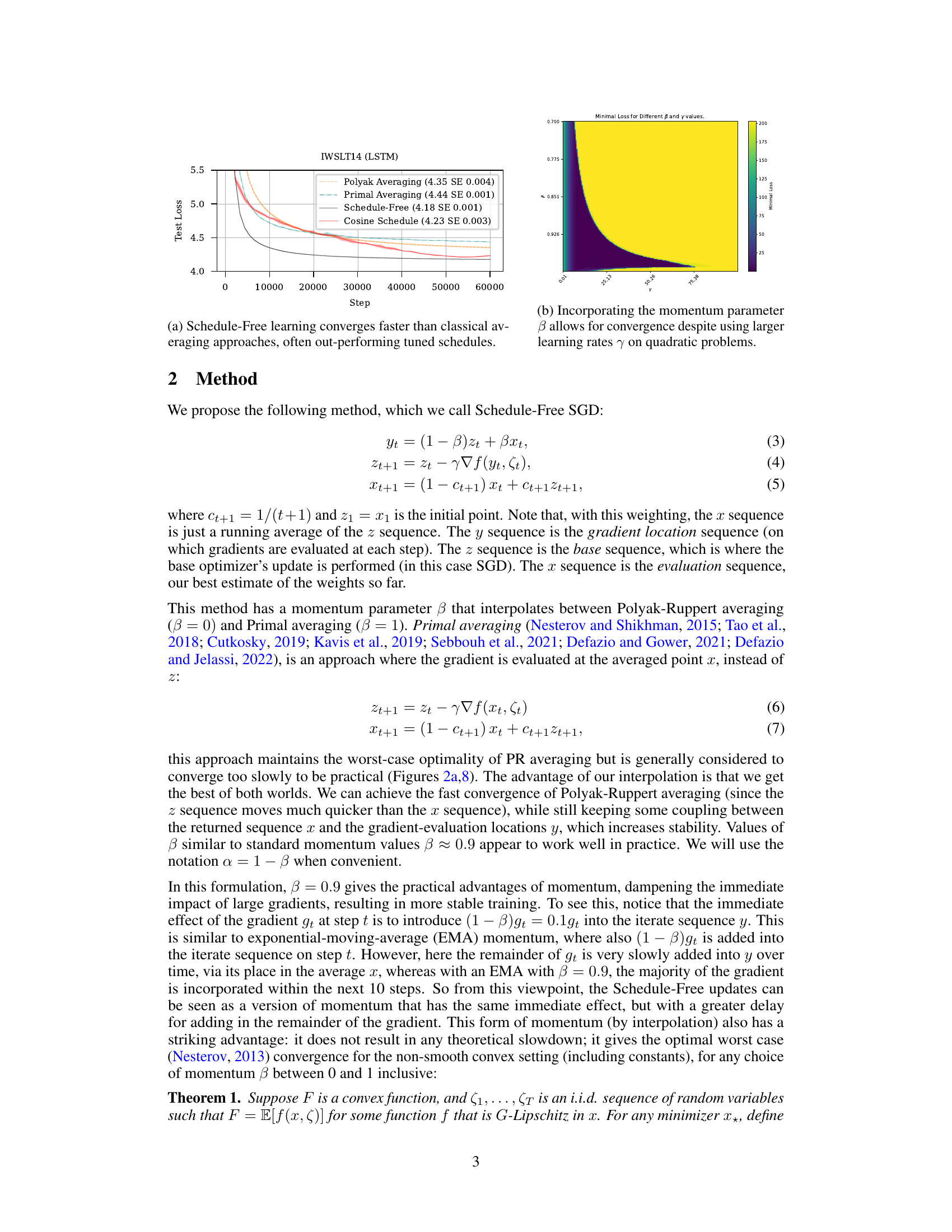
This figure shows the training performance of Schedule-Free SGD and Schedule-Free AdamW compared to traditional cosine learning rate schedules. The black lines represent the Schedule-Free methods, demonstrating that they closely follow the Pareto frontier (optimal balance between loss and training time). The red lines represent cosine schedules with different lengths. The results show that Schedule-Free methods perform comparably to or better than the tuned cosine schedules, even without requiring the specification of the optimization stopping time.
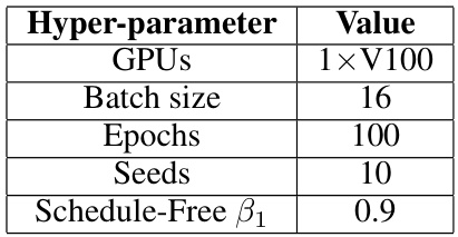
This table shows the hyperparameter settings used for the convex problem experiments in the paper. It lists the number of GPUs used, batch size, number of epochs, number of random seeds used, and the beta1 parameter for the Schedule-Free optimizer.
In-depth insights#
Schedule-Free Optimizers#
Schedule-free optimizers represent a significant departure from traditional optimization approaches by eliminating the need for pre-defined learning rate schedules. This innovative strategy offers several key advantages. Firstly, it simplifies the optimization process by removing the hyperparameter tuning burden associated with selecting and configuring schedules. Secondly, by removing the reliance on a pre-defined schedule, the training process becomes more adaptive, adjusting its learning rate dynamically based on the current state of the optimization. This adaptability can lead to improved performance and faster convergence, especially for complex, non-convex problems. Thirdly, schedule-free optimizers often demonstrate improved efficiency, achieving comparable or even superior results with less hyperparameter tuning, potentially reducing computational costs and time.
Large Learning Rates#
The section on “Large Learning Rates” challenges conventional wisdom in optimization theory. Classical theory suggests that using large learning rates leads to suboptimal convergence. However, empirical results consistently show that larger learning rates yield superior performance, contradicting theoretical predictions. The authors investigate a specific case where large learning rates achieve optimal convergence rates up to constant factors. This finding is significant because it bridges the gap between theory and practice, demonstrating that current theoretical frameworks may be insufficient to fully capture the complexities of modern machine learning optimization. This work also highlights the need for more nuanced theoretical models that can explain the effectiveness of large learning rates in various problem settings and algorithms.
Theoretical Unification#
A theoretical unification in machine learning typically involves connecting seemingly disparate concepts or algorithms under a single, overarching framework. This often reveals hidden relationships, improves understanding, and enables the development of more powerful and generalizable methods. In the context of optimization, such a unification might connect learning rate schedules and iterate averaging, perhaps by showing that one can be derived from or is a special case of the other. This unified perspective could lead to improved optimization algorithms, ones that automatically adapt to problem characteristics without requiring manual tuning of hyperparameters like the learning rate schedule. A strong unification would not only explain existing methods but also suggest new, improved ones, potentially bridging the gap between theoretical optimality and practical performance often seen in machine learning. Furthermore, a successful unification would streamline the field by presenting a coherent and simplified theoretical landscape.
Empirical Evaluation#
An Empirical Evaluation section in a research paper would ideally present a robust and detailed examination of the proposed method’s performance. It should go beyond simply reporting metrics; instead, it should offer insightful analysis of the results, exploring various aspects such as the method’s sensitivity to hyperparameters, its generalizability across different datasets or problem instances, and comparisons to existing state-of-the-art techniques. A strong emphasis on clear visualizations and well-chosen metrics is vital for effective communication. The discussion should carefully consider potential limitations and biases, providing a balanced and nuanced perspective. Statistical significance testing should be applied, where appropriate, to validate the observed differences in performance. Ideally, the experiments would be carefully designed to control confounding variables and ensure the reliability of the findings. In short, a well-crafted Empirical Evaluation section builds trust in the proposed method by demonstrating its effectiveness and offering valuable insights for future research.
Future Research#
Future research directions stemming from this Schedule-Free optimization approach could explore several promising avenues. Extending the theoretical framework to encompass broader classes of problems beyond convex and Lipschitz functions is crucial. This involves investigating the behavior and convergence properties of Schedule-Free methods in non-convex settings and under various noise models, potentially leveraging tools from non-convex optimization theory. Empirical evaluations on a wider range of deep learning architectures and datasets would strengthen the claims of generalizability. This includes exploring the impact of varying model sizes and complexities, comparing its performance against other state-of-the-art optimizers across diverse benchmarks, and analyzing performance on resource-constrained settings. Investigating the underlying reasons for the superior empirical performance observed despite theoretically suboptimal learning rates warrants in-depth analysis. This involves a deeper examination of the interplay between momentum, averaging, and learning rate schedules, potentially uncovering novel insights into optimization dynamics. Finally, developing practical strategies for hyperparameter tuning could significantly enhance the usability of the method, with a focus on automated techniques to achieve near-optimal performance across various problem instances.
More visual insights#
More on figures
This figure shows the performance of Schedule-Free SGD and Schedule-Free AdamW compared to cosine learning rate schedules. Both Schedule-Free methods track the Pareto frontier (optimal balance between training time and loss) closely. In both the left and right panels, the Schedule-Free method matches or surpasses the performance of the cosine schedules.
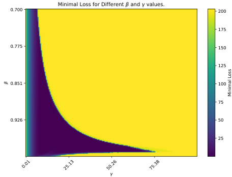
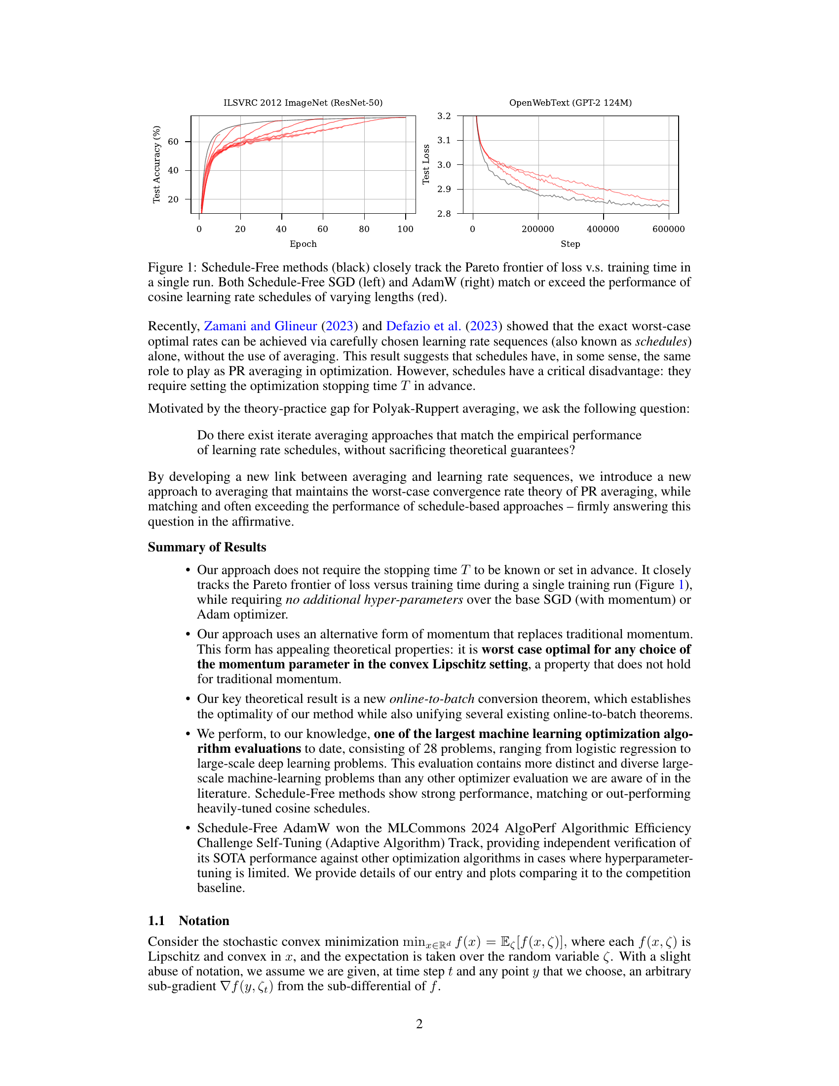
The figure is a heatmap showing the minimal loss achieved as a function of the two parameters β (momentum parameter) and γ (learning rate). The x-axis represents different values of γ, and the y-axis represents different values of β. The color of each cell in the heatmap indicates the minimal loss achieved for the given values of β and γ. The heatmap reveals that when the learning rate γ is small, the value of β has little effect on the convergence of the algorithm. However, when γ is large, choosing β < 1 becomes crucial for achieving convergence.
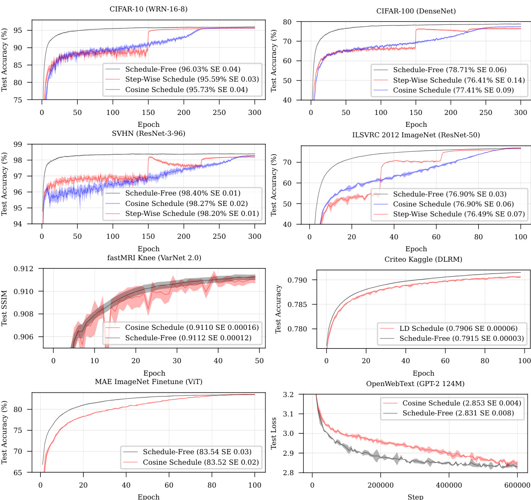
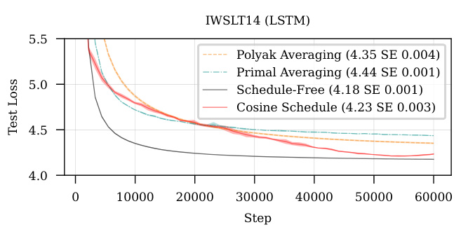
This figure presents the results of deep learning experiments comparing the performance of Schedule-Free methods against traditional cosine learning rate schedules and step-wise schedules across various benchmark datasets and architectures. The results demonstrate that Schedule-Free methods consistently match or exceed the performance of the other methods, highlighting the efficacy of the proposed approach. The datasets include CIFAR-10, CIFAR-100, SVHN, ImageNet, IWSLT14, fastMRI, Criteo Kaggle, and OpenWebText. The architectures range from relatively simple convolutional neural networks to complex Transformers.
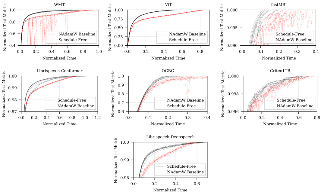
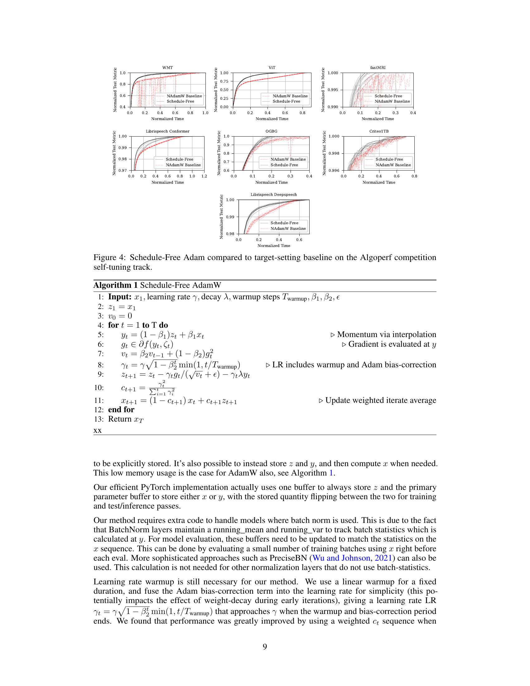
This figure compares the performance of Schedule-Free AdamW against the NAdamW baseline in the MLCommons AlgoPerf Algorithmic Efficiency Challenge Self-Tuning track. The figure presents normalized test metrics (y-axis) against normalized time (x-axis) across eight different deep learning tasks: WMT, ViT, fastMRI, Librispeech Conformer, OGBG, Criteo1TB, Librispeech Deepspeech. Each task is presented as a separate subplot. The black lines represent the performance of Schedule-Free AdamW across ten different random seeds. The red dotted line shows the NAdamW baseline. The results indicate that Schedule-Free AdamW generally matches or exceeds the performance of the NAdamW baseline across various tasks.

This figure compares the performance of Schedule-Free methods against cosine learning rate schedules and step-wise schedules on various deep learning tasks. The results show that Schedule-Free methods closely track the Pareto frontier of loss vs. training time, often matching or exceeding the performance of tuned schedules across a range of problems, including image classification, translation, and natural language processing.
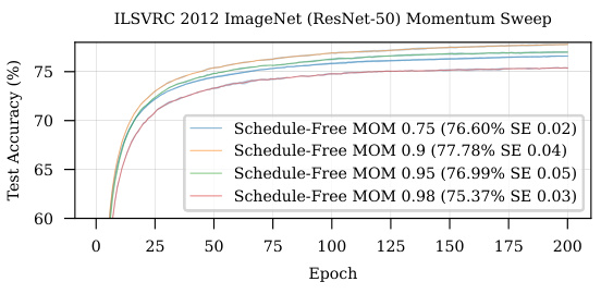
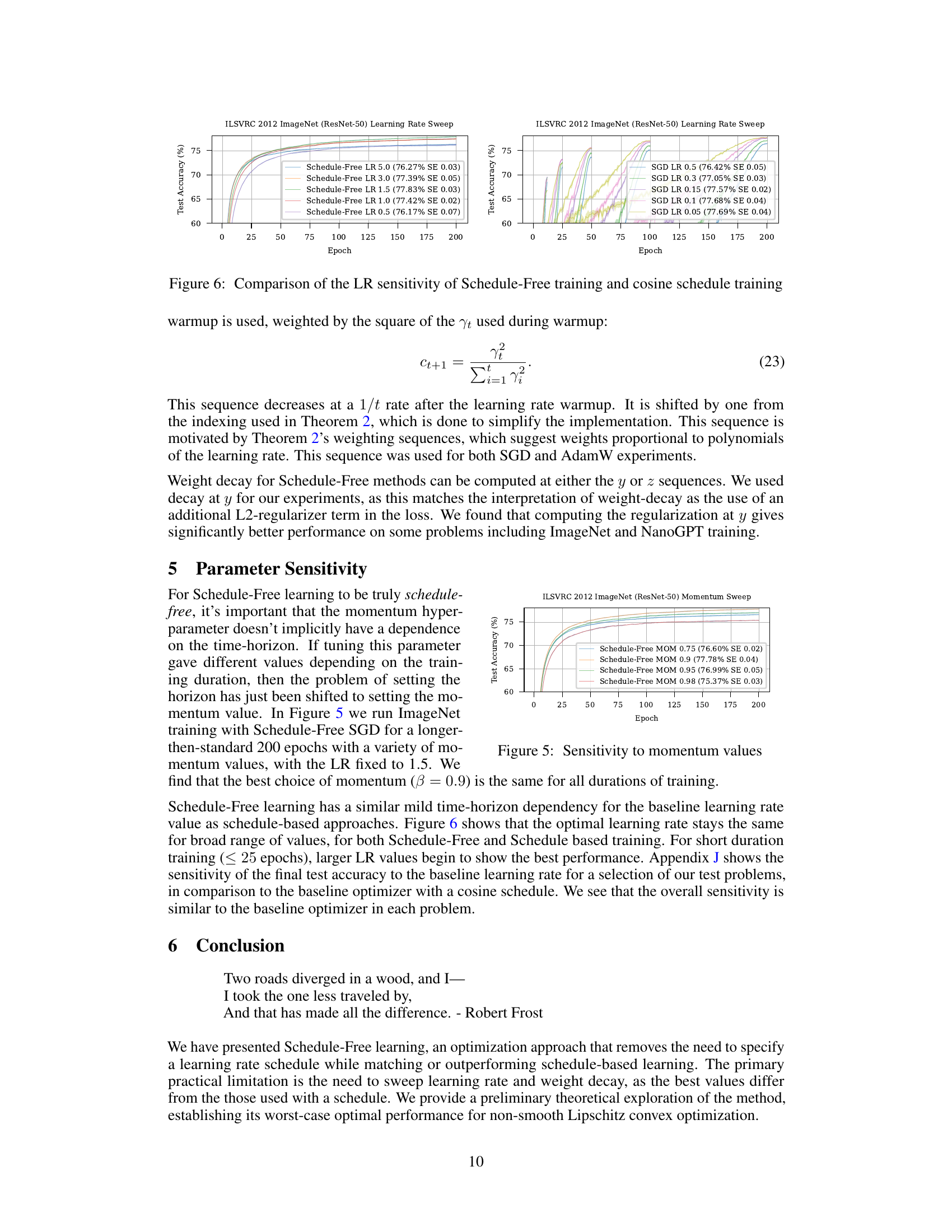
The figure shows the impact of different momentum values (β) on the convergence of the Schedule-Free method. It uses ImageNet ResNet-50 training for 200 epochs with a fixed learning rate of 1.5. The results indicate that the optimal momentum value (β=0.9) remains consistent across different training durations, demonstrating the time-horizon independence of this hyperparameter in Schedule-Free learning.
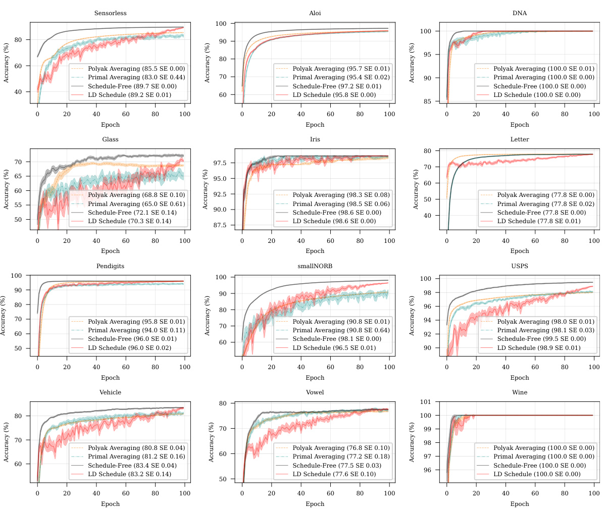
This figure shows the results of stochastic logistic regression experiments, comparing the performance of Polyak averaging, primal averaging, Schedule-Free, and a linear decay schedule across twelve different datasets. Each subplot represents a dataset and shows the accuracy over epochs for each method. The results visually demonstrate the superior performance of the Schedule-Free approach across several datasets.
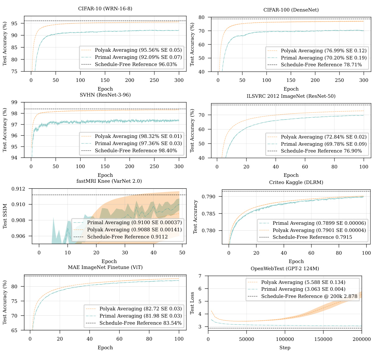
This figure compares the performance of Polyak averaging, primal averaging, and the Schedule-Free method on various deep learning tasks. Each subplot shows the test accuracy or loss over epochs for a specific task. The results demonstrate that the Schedule-Free method generally matches or exceeds the performance of the other averaging methods, indicating its effectiveness across diverse machine learning problems.
The figure shows the performance comparison of Schedule-Free methods against cosine learning rate schedules and step-wise schedules on various deep learning tasks, including CIFAR-10, CIFAR-100, SVHN, ImageNet, IWSLT14, fastMRI, Criteo DLRM, and OpenWebText. The results demonstrate that Schedule-Free methods closely track the Pareto frontier of loss versus training time and often outperform tuned schedules.
More on tables
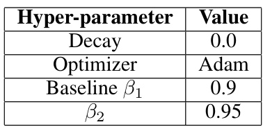
This table presents the hyperparameter settings used in the convex experiments. It shows the values used for the decay, optimizer, and beta parameters (β1 and β2). These parameters are crucial components of the optimization algorithms used in the paper, and their settings influence the performance and convergence.

This table presents the results of deep learning experiments comparing Schedule-Free AdamW against the baseline methods and cosine schedule for various tasks like CIFAR-10, CIFAR-100, SVHN, ImageNet, IWSLT14, fastMRI, Criteo, and OpenWebText. It demonstrates that Schedule-Free methods often outperforms other methods in terms of test accuracy or loss.

This table shows the hyperparameters used for the CIFAR-100 experiment. It includes architectural details (DenseNet), training parameters (epochs, GPUs, batch size, warmup percentage), optimization settings (Schedule-Free β, learning rates for both Schedule-Free and Cosine approaches, decay, momentum), and other details like the number of seeds used.

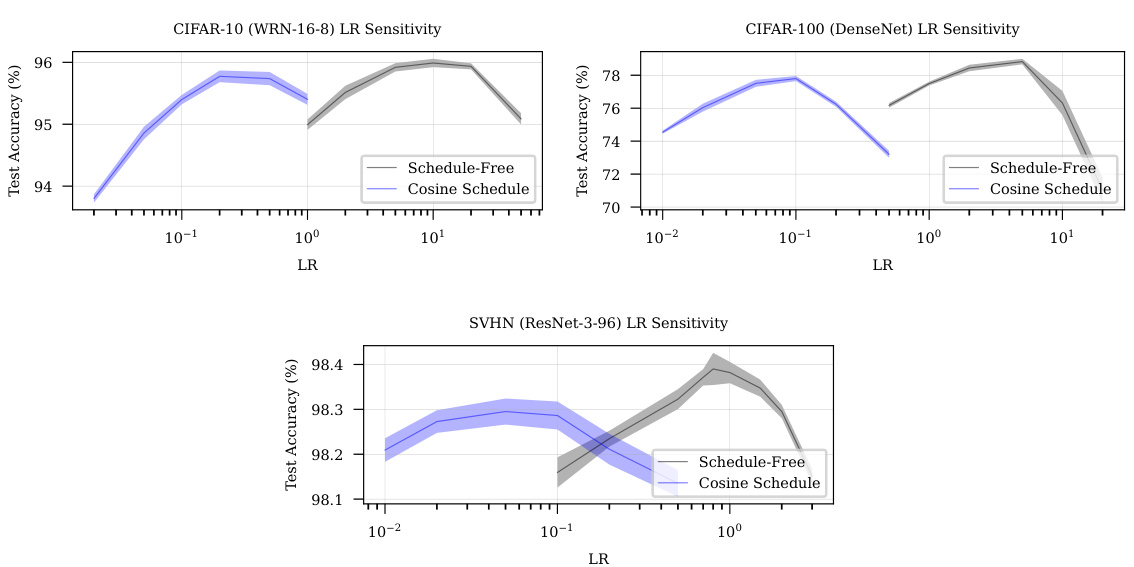
This table compares the sensitivity of learning rate for Schedule-Free training and cosine schedule training on the ImageNet dataset using ResNet-50 architecture. It shows the test accuracy obtained at different learning rates (0.5, 1.0, 1.5, 3.0, 5.0) for both approaches over 200 epochs. The results highlight that schedule-free training displays a broader range of optimal learning rates, indicating robustness and less sensitivity to hyperparameter tuning.

This table compares the sensitivity of the learning rate (LR) for Schedule-Free training and cosine schedule training. It shows how different learning rates affect the performance of both methods. The comparison is important for understanding how the hyperparameters of the two methods affect their performance.
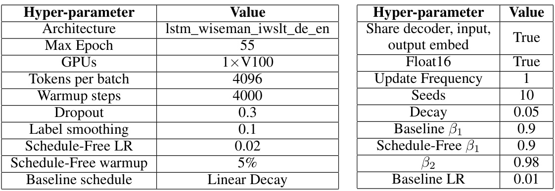
This table compares the sensitivity of Schedule-Free and Cosine training methods to different learning rates. It shows how the test accuracy changes for both methods with variations in the learning rate across several epochs, illustrating the relative robustness and optimal learning rate ranges for each approach.
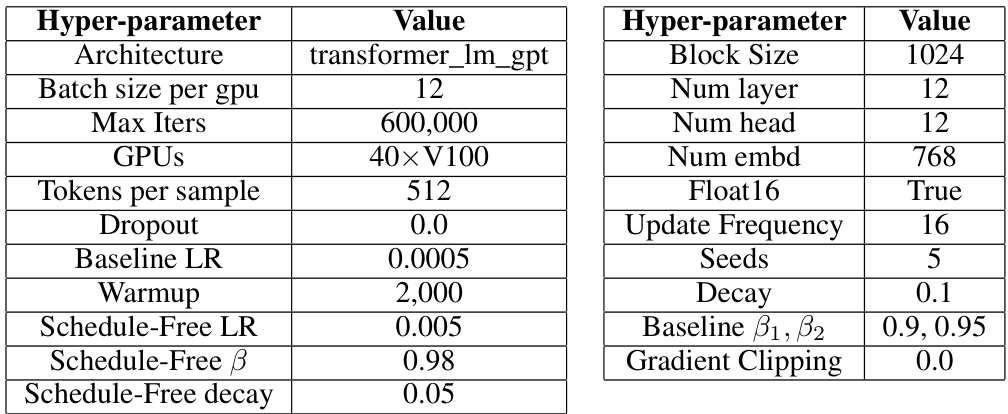
This figure compares the performance of Schedule-Free AdamW against a target-setting NAdamW baseline across various tasks in the MLCommons AlgoPerf Algorithmic Efficiency Challenge Self-Tuning track. The plots show the normalized test metric (y-axis) against normalized time (x-axis) for each task, illustrating the relative performance of both algorithms in terms of achieving target metrics within a given timeframe.

This table shows the sensitivity analysis of learning rate for both the Schedule-Free training and cosine schedule training on ImageNet dataset. The results are presented in terms of test accuracy with respect to various learning rates. The data demonstrates the performance of both methods across a range of learning rates, highlighting the relative robustness and effectiveness of each approach.

This figure shows the sensitivity of Schedule-Free SGD performance on ImageNet to different momentum values (β). The experiment uses a fixed learning rate of 1.5 and trains for 200 epochs. It demonstrates that the optimal momentum parameter is consistent across various training durations, indicating that it is not implicitly dependent on the training horizon.

This table shows the hyperparameter settings used for the MRI experiment. It lists the architecture, epochs, GPUs used, batch size per GPU, acceleration factor, baseline schedule, baseline learning rate, beta2 value, low frequency lines, mask type, seeds, decay, baseline beta1, Schedule-Free learning rate, and Schedule-Free beta values.

This table shows the hyperparameter settings used for the Schedule-Free AdamW submission to the MLCommons AlgoPerf Algorithmic Efficiency Challenge Self-Tuning track. It lists the values for learning rate, one-minus Beta1, Beta2 (default), weight decay (default), dropout rate, warmup percentage, label smoothing, and polynomial in ct average.
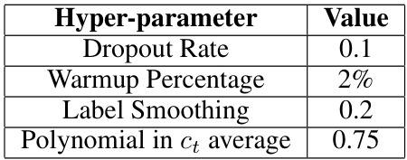
This table lists the hyper-parameters used for the Schedule-Free AdamW submission to the MLCommons 2024 AlgoPerf Algorithmic Efficiency Challenge Self-Tuning track. The self-tuning track required that a single set of hyper-parameters be used for all problems, making the choice of good defaults especially important. The hyper-parameters listed represent a good default configuration for a broad range of deep learning problems.
Full paper#
