↗ OpenReview ↗ NeurIPS Proc. ↗ Chat
TL;DR#
Training neural networks with loss functions involving high-dimensional and high-order differential operators is computationally expensive due to the scaling of derivative tensor size and computation graph. Existing methods like Stochastic Dimension Gradient Descent (SDGD) address this through randomization, while high-order auto-differentiation (AD) handles the exponential scaling for univariate functions. However, neither method effectively handles both high dimensionality and high-order derivatives simultaneously.
This paper introduces the Stochastic Taylor Derivative Estimator (STDE), which efficiently addresses these challenges. STDE leverages univariate high-order AD by intelligently constructing input tangents, allowing for efficient contraction of derivative tensors and randomization of arbitrary differential operators. The method demonstrates significant speedup and memory reduction over existing techniques when applied to Physics-Informed Neural Networks (PINNs), solving 1-million-dimensional PDEs in just 8 minutes on a single GPU.
Key Takeaways#
Why does it matter?#
This paper is crucial for researchers working with high-dimensional and high-order differential operators, especially in areas like physics-informed machine learning. It provides a significant speedup and memory reduction, opening avenues for tackling complex real-world problems previously intractable due to computational limitations. The method presented, STDE, is applicable to various differential operators, furthering the development of efficient techniques for solving PDEs in high-dimensional settings. This work directly addresses current challenges in scientific computing and machine learning, paving the way for new solutions and innovations.
Visual Insights#

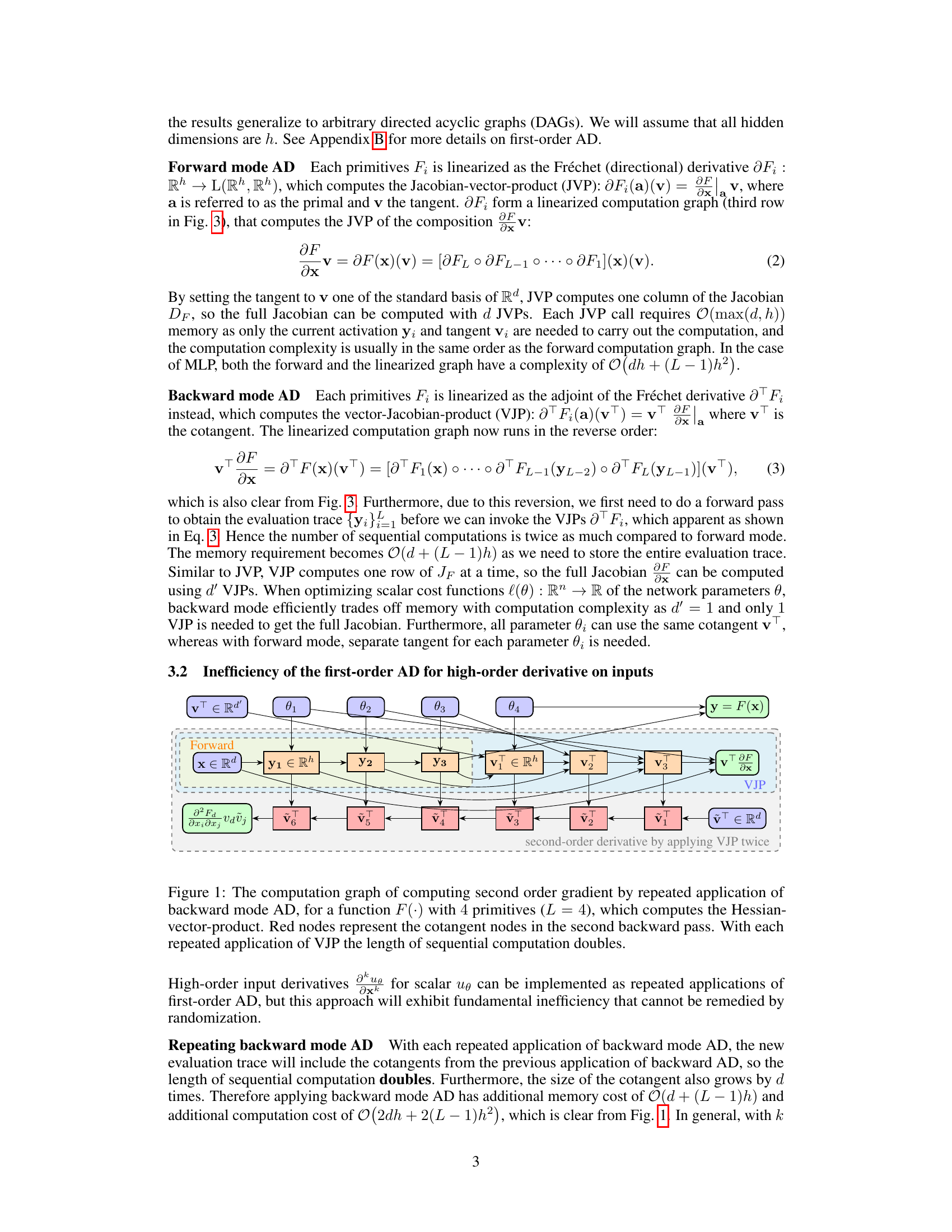
This figure illustrates the inefficiency of using repeated backward mode automatic differentiation (AD) for higher-order derivatives. It shows that with each repeated application of the backward pass (VJP), the computation graph grows exponentially in length and memory usage. The red nodes highlight the accumulating cotangents in the second backward pass, emphasizing the computational cost increase.

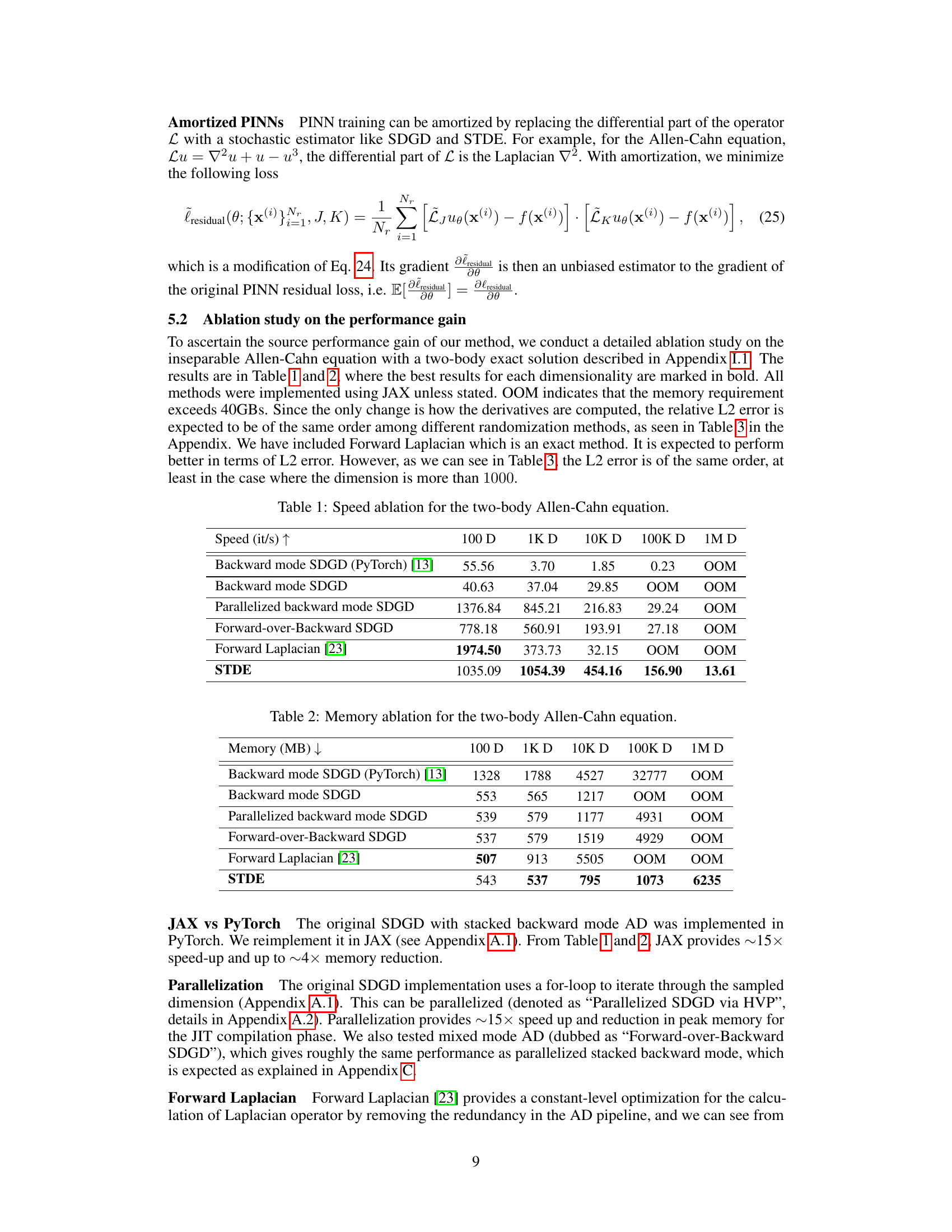
This table presents a speed comparison of different methods for solving the two-body Allen-Cahn equation across varying dimensions (100D to 1M D). The methods compared include backward mode SDGD (using PyTorch and JAX), parallelized backward mode SDGD, forward-over-backward SDGD, forward Laplacian, and the proposed STDE. The table shows the iterations per second (it/s) achieved by each method for each dimension, highlighting the significant speedup achieved by STDE, particularly in higher dimensions.
In-depth insights#
STDE: Efficient Amortization#
The concept of “STDE: Efficient Amortization” centers on addressing the computational challenges of optimizing neural networks with loss functions involving high-dimensional and high-order differential operators. Traditional backpropagation methods suffer from exponential scaling in both dimensionality and derivative order. STDE mitigates this by amortizing the computation of these expensive operators over the optimization process through randomization. This clever approach leverages high-order automatic differentiation (AD) to efficiently contract derivative tensors, even for multivariate functions. The method cleverly constructs input tangents for univariate high-order AD, enabling the efficient randomization of arbitrary differential operators. The core innovation lies in using properly constructed input tangents to univariate high-order AD to achieve efficient contraction of higher-order derivative tensors for multivariate functions. This is a significant improvement over existing methods, offering substantial speed-ups and memory savings, as demonstrated by its application to Physics-Informed Neural Networks (PINNs), where it enabled solving previously intractable 1-million-dimensional PDEs. STDE generalizes and subsumes previous methods, unifying seemingly disparate approaches under a single framework. The efficacy of the method and the source of its performance gain is well-validated through a comprehensive experimental ablation study.
High-Order AD Application#
High-order automatic differentiation (AD) offers a powerful technique for efficiently computing higher-order derivatives, which are crucial in various applications involving complex functions. Its application to solving high-dimensional partial differential equations (PDEs) is particularly impactful, as traditional methods often struggle with the computational cost and memory requirements associated with high dimensionality and high-order derivatives. High-order AD enables the approximation of these derivatives directly within neural networks, accelerating the optimization process. This is especially beneficial when dealing with loss functions incorporating high-order differential operators, like those found in physics-informed neural networks (PINNs). However, challenges remain in scaling high-order AD to very high-dimensional problems, due to the exponential growth in computational complexity. Techniques like randomization and sparse tensor computations are vital in mitigating this issue, allowing for the practical application of high-order AD in large-scale scientific computing and machine learning tasks. Further research should focus on developing more efficient and scalable algorithms, particularly for handling complex, non-linear differential operators common in real-world applications.
STDE Generalization#
The concept of “STDE Generalization” in the context of a research paper likely refers to the extent to which the Stochastic Taylor Derivative Estimator (STDE) method can be applied to a broader range of problems beyond those initially demonstrated. A thoughtful exploration would analyze how the core principles of STDE, efficiently contracting high-order derivative tensors via properly constructed input tangents to univariate high-order AD, can be extended. This involves examining its adaptability to diverse differential operators, going beyond simple examples, and assessing its performance across varying problem dimensions and complexities. Generalization would also include considering different types of PDEs and their associated operators, exploring the impact of varying levels of sparsity and non-linearity in the operator on STDE’s efficiency and accuracy. Furthermore, a key aspect would be evaluating the impact of the chosen randomization strategies on the overall estimator’s variance, aiming to minimize error while maintaining computational efficiency. A generalized STDE would ideally offer a robust and versatile framework for high-dimensional and high-order differential equation solutions, paving the way for its utilization in a significantly wider range of scientific and engineering applications.
PINN Speedup#
The concept of “PINN Speedup” in the context of a research paper likely revolves around enhancing the computational efficiency of Physics-Informed Neural Networks (PINNs). PINNs, while powerful for solving partial differential equations (PDEs), often suffer from high computational costs, especially when dealing with high-dimensional problems. A significant speedup would likely be achieved by employing techniques that accelerate the training process. This could involve optimizing the neural network architecture, perhaps through specialized layers or connections designed for PDEs. Another approach might be to leverage advanced optimization algorithms that converge faster. Stochastic methods, such as those employing random sampling, are also viable options for reducing computational complexity by approximating difficult-to-compute quantities. Importantly, a speedup claim must be supported by empirical evidence showing a substantial reduction in training time or computational resources compared to a suitable baseline method. The level of speedup achieved should also be carefully contextualized considering factors like problem dimensionality, the specific PDE being solved, and the hardware used.
Future Work: Variance#
Analyzing variance in stochastic methods is crucial for reliable estimations. Future work should investigate variance reduction techniques applicable to the Stochastic Taylor Derivative Estimator (STDE), such as control variates or importance sampling. The impact of batch size on variance needs further study; smaller batches offer computational advantages but may increase variance, necessitating a careful trade-off analysis. Theoretical bounds on the variance of STDE for various operators and input distributions would provide valuable insights into its reliability and efficiency. Furthermore, comparing the variance of STDE with other methods like SDGD and Hutchinson’s trace estimator across different problem settings and scales will reveal its strengths and weaknesses. Such a comprehensive analysis would strengthen the practical applicability of STDE and guide future improvements.
More visual insights#
More on figures

This figure illustrates the computation graph for calculating the second-order Fréchet derivative (d²F) of a function F composed of four primitives (F1 to F4). The input is a 2-jet, which contains the primal (x) and two tangents (v(1) and v(2)). Each primitive’s second-order derivative is applied sequentially, pushing the 2-jet forward through the computation graph. The key point is that each row of the computation can be done in parallel, unlike traditional methods, and no evaluation trace needs to be stored, making this approach significantly more memory-efficient and computationally faster.

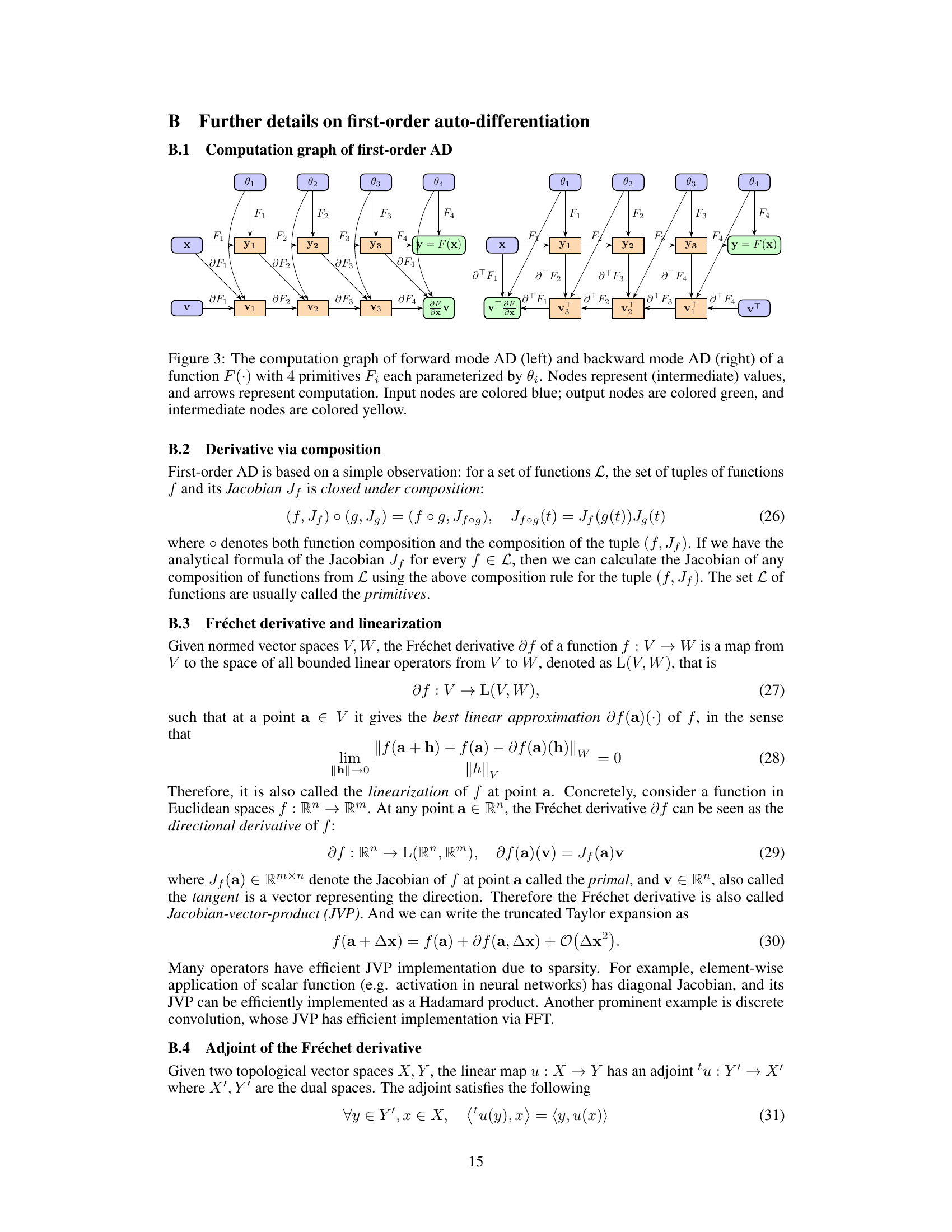
This figure illustrates the computation graphs for both forward and backward mode automatic differentiation (AD). The forward mode computes the Jacobian-vector product (JVP) by propagating a tangent vector through the linearized computation graph. The backward mode computes the vector-Jacobian product (VJP) by propagating a cotangent vector backward through the adjoint linearized graph. The figure highlights the differences in computational flow and memory requirements between the two methods.
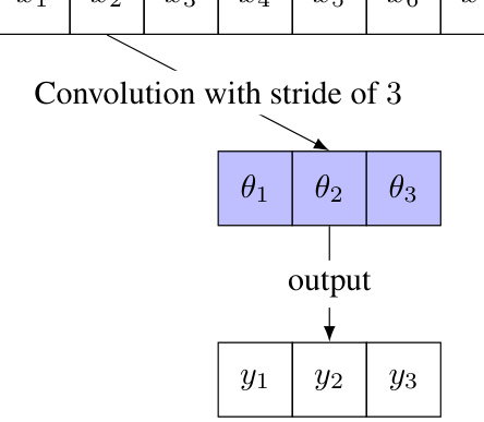
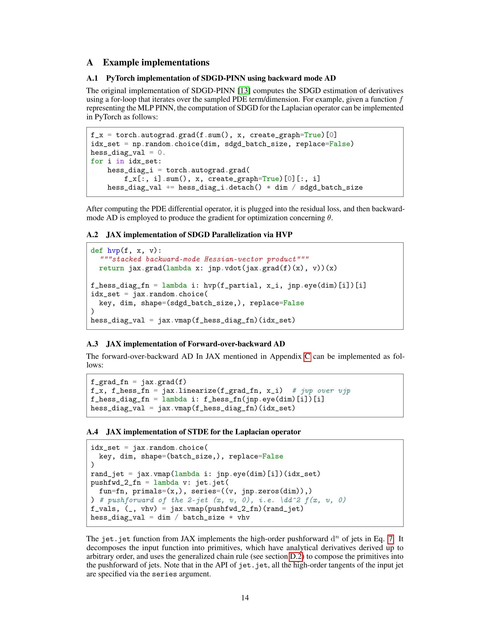
This figure illustrates the concept of convolutional weight sharing in the first layer of a neural network. The input has a dimension of 9. A 1D convolution with a filter size of 3 and a stride of 3 is applied. This reduces the number of parameters, since the same weights (θ₁, θ₂, θ₃) are used across multiple input elements (x₁, x₂, x₃; x₄, x₅, x₆; x₇, x₈, x₉). The output of the convolution are three elements (y₁, y₂, y₃). This technique is employed to handle high-dimensional input data efficiently, reducing the memory footprint during the training process.
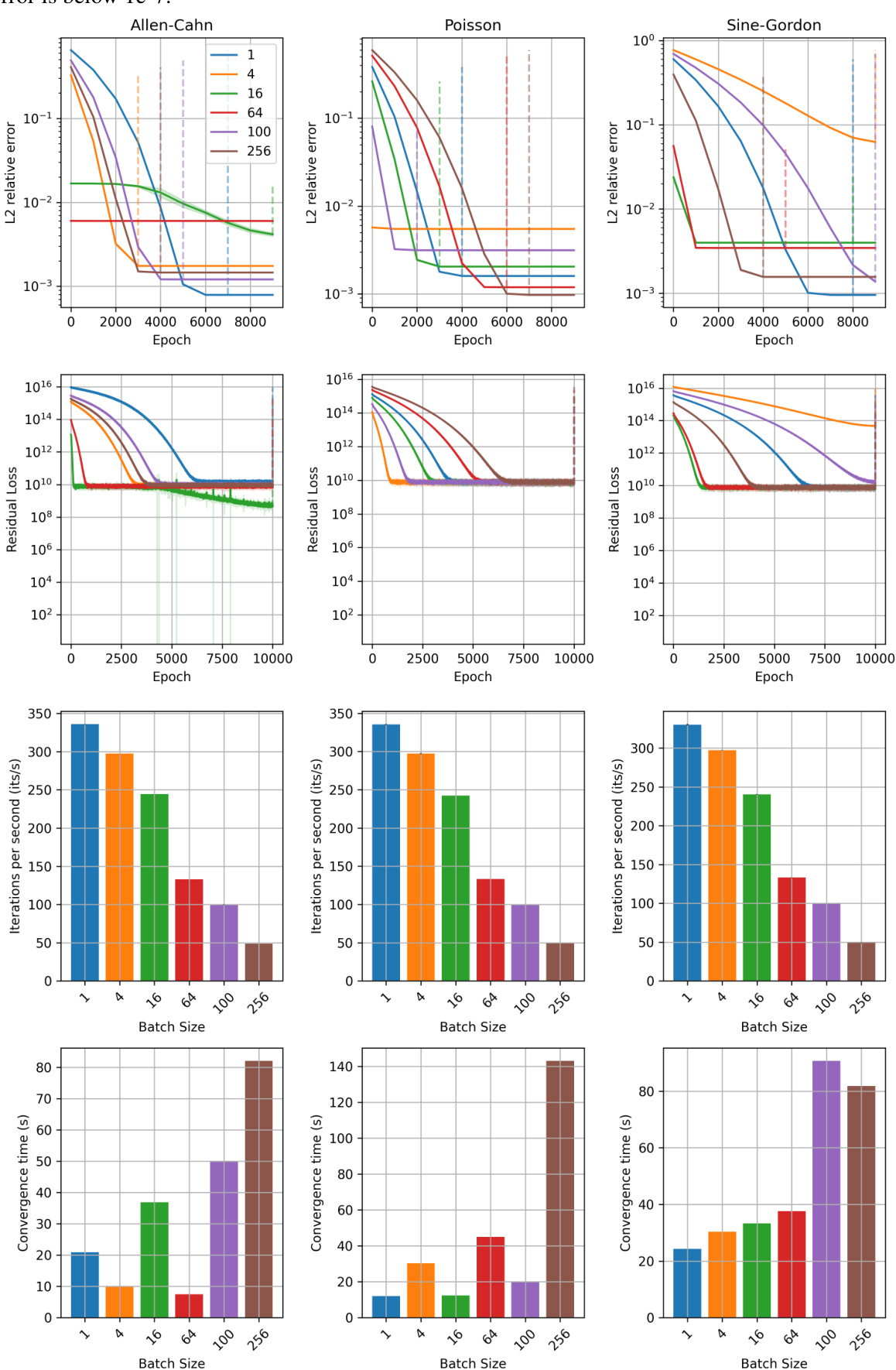
This figure displays ablation studies on the impact of randomization batch size on the performance of the proposed method (STDE) for solving three different types of PDEs: Allen-Cahn, Poisson, and Sine-Gordon. The results are shown across various metrics including L2 relative error, residual loss, iterations per second, and convergence time. Each sub-figure presents these metrics for a specific PDE, demonstrating how changes in batch size affect the model’s convergence behavior and overall efficiency. The consistent pattern across PDE types emphasizes the impact of this hyperparameter.
More on tables

This table shows the memory usage (in MB) of different methods for solving the two-body Allen-Cahn equation with varying dimensionality (100D, 1K D, 10K D, 100K D, 1M D). The methods compared include Backward mode SDGD using PyTorch and JAX, Parallelized backward mode SDGD, Forward-over-Backward SDGD, Forward Laplacian, and STDE. The table highlights the significant memory reduction achieved by STDE, especially as the dimensionality increases.

This table presents a comparison of different methods for solving the Inseparable Allen-Cahn equation with a two-body exact solution. It compares the speed (iterations per second), memory usage (in MB), and error (L2 relative error) for several methods: Backward mode SDGD (using PyTorch and JAX), Parallelized backward mode SDGD, Forward-over-Backward SDGD, Forward Laplacian, and STDE (with and without a batch size of 16). The results are shown for different input dimensions (100D, 1K D, 10K D, 100K D, and 1M D), illustrating the performance and scalability of each method. The table highlights the significant speedup and memory reduction achieved by the STDE method, especially at higher dimensions.

This table presents a comparison of different methods for solving the Inseparable Allen-Cahn equation using PINNs. The methods compared include backward mode SDGD (both PyTorch and JAX implementations), parallelized backward mode SDGD, forward-over-backward SDGD, forward Laplacian, and STDE (with and without a smaller batch size). The table shows the speed (iterations per second), memory usage (in MB), and L2 relative error for each method across different dimensions (100D, 1K D, 10K D, 100K D, and 1M D). The results highlight the significant speed and memory improvements achieved by STDE, particularly at higher dimensions, compared to the other methods. Note that OOM indicates that the memory requirement exceeded 40GB. The results demonstrate the effectiveness and scalability of STDE for solving high-dimensional PDEs.

This table presents the computational results for the Inseparable Allen-Cahn equation using different methods. It compares the speed (iterations per second), memory usage (in MB), and error (L2 relative error) for various dimensionalities (100D, 1K D, 10K D, 100K D, 1M D) using Backward mode SDGD (PyTorch and JAX), Parallelized backward mode SDGD, Forward-over-Backward SDGD, Forward Laplacian, and STDE (with and without batch size = 16). The results show STDE’s superior performance in terms of both speed and memory efficiency compared to other methods, especially at higher dimensions.
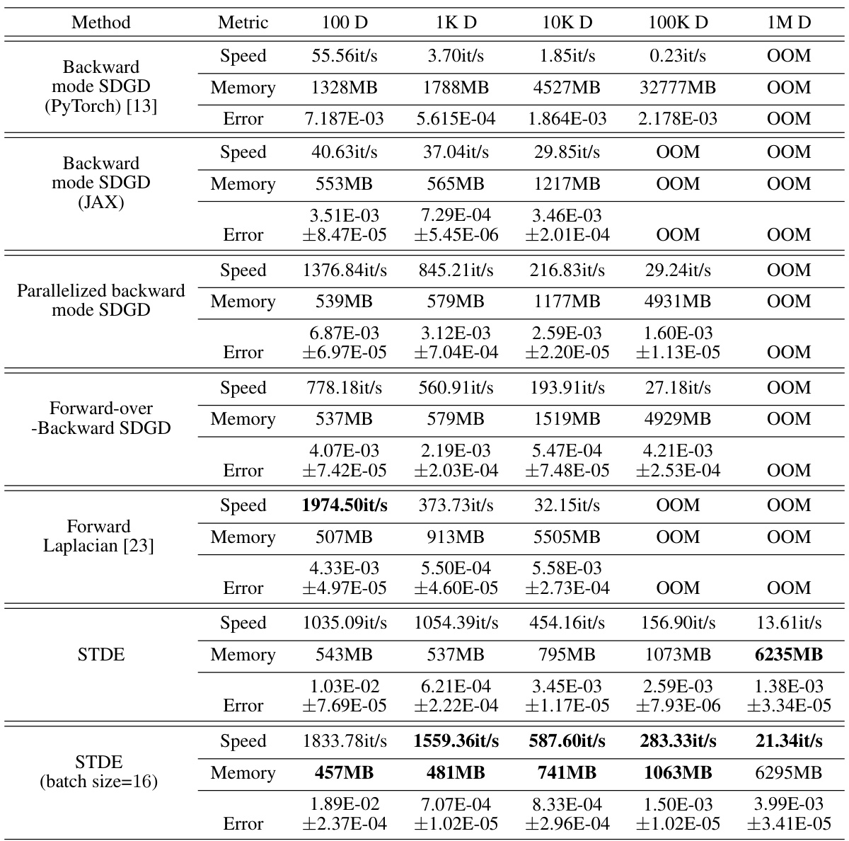
This table presents the computational results for the Inseparable Allen-Cahn equation using different methods. It compares the speed (iterations per second), memory usage (in MB), and error (L2 relative error with standard deviation) across various dimensionalities (100D, 1K D, 10K D, 100K D, 1M D). The methods compared include backward mode SDGD (using PyTorch and JAX), parallelized backward mode SDGD, forward-over-backward SDGD, forward Laplacian, and STDE (with and without a smaller batch size). The table highlights the efficiency gains of STDE, especially at higher dimensions.

This table presents a comparison of different methods for solving the Inseparable Allen-Cahn equation with a two-body exact solution. It shows the speed (iterations per second), memory usage (MB), and error (L2 relative error) for various dimensionalities (100D, 1K D, 10K D, 100K D, 1M D). The methods compared include Backward mode SDGD (using PyTorch and JAX), Parallelized backward mode SDGD, Forward-over-Backward SDGD, Forward Laplacian, and STDE (with and without a batch size of 16). The results highlight the efficiency gains of STDE, particularly in higher dimensions.

This table presents a comparison of different methods for solving the Inseparable Allen-Cahn equation with a two-body exact solution. The methods compared include Backward mode SDGD (using PyTorch and JAX), Parallelized backward mode SDGD, Forward-over-Backward SDGD, Forward Laplacian, and STDE (with and without a smaller batch size). For each method, the table shows the speed (iterations per second), memory usage (in MB), and the L2 relative error. The results are shown for different input dimensions (100D, 1K D, 10K D, 100K D, and 1M D).
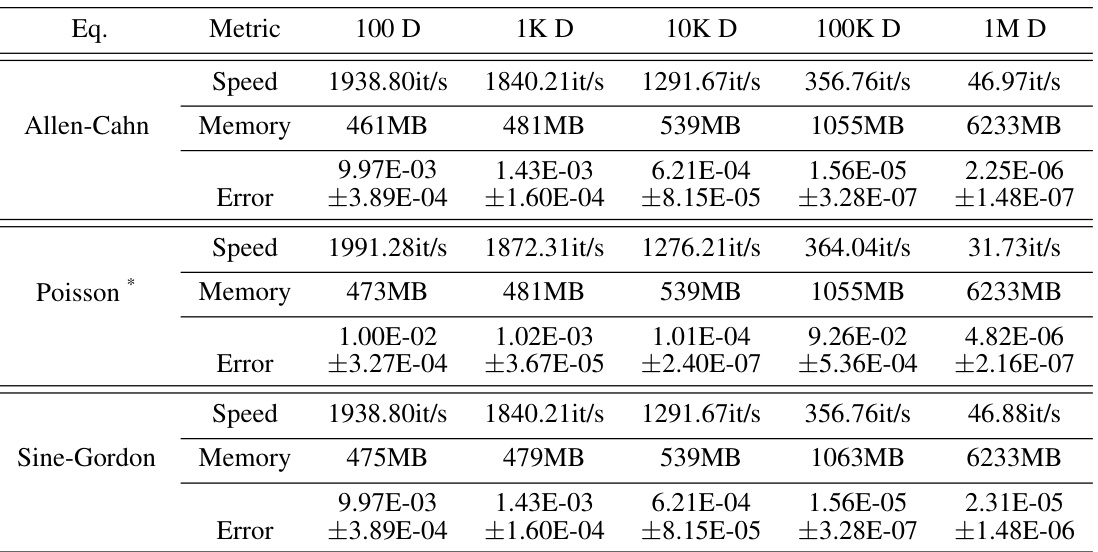
This table presents a comparison of different methods for solving the Inseparable Allen-Cahn equation with a two-body exact solution. The methods compared include Backward mode SDGD (using PyTorch and JAX), Parallelized backward mode SDGD, Forward-over-Backward SDGD, Forward Laplacian, and STDE (with and without a batch size of 16). The table shows the speed (iterations per second), memory usage (in MB), and the relative L2 error for each method across different input dimensions (100D, 1K D, 10K D, 100K D, and 1M D). The results highlight the performance improvements achieved by STDE, particularly in terms of speed and memory efficiency, especially as the dimensionality of the problem increases.
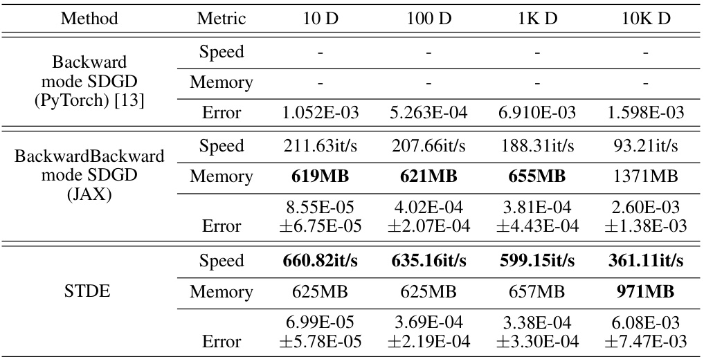
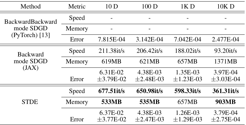
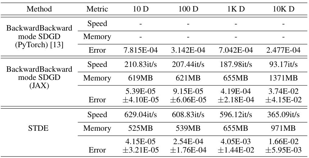
This table presents the results of the Time-dependent Semilinear Heat equation experiments. It compares the performance of three methods: Backward mode SDGD (PyTorch), Backward mode SDGD (JAX), and STDE. The metrics shown are speed, memory usage, and error. The number of sampled dimensions for SDGD is consistently set to 10, allowing for a comparison across different dimensionalities (10D, 100D, 1KD, 10KD).
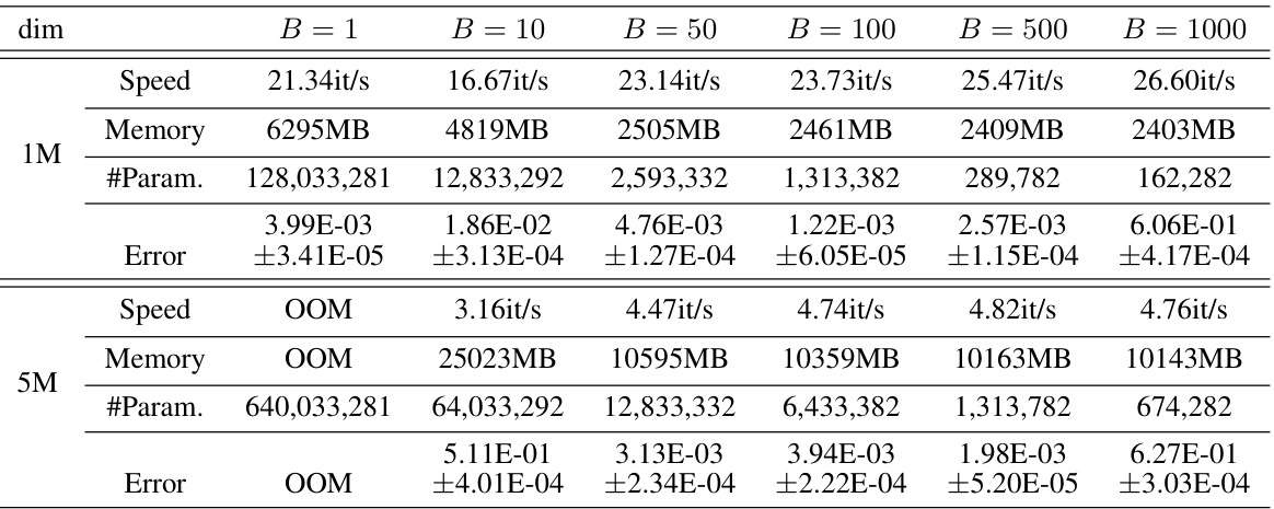
This table presents a comparison of different methods for solving the Inseparable Allen-Cahn equation with a two-body exact solution. The methods compared include Backward mode SDGD (using both PyTorch and JAX), Parallelized backward mode SDGD, Forward-over-Backward SDGD, Forward Laplacian, and STDE (with and without a smaller batch size). The table shows the speed (iterations per second), memory usage (in MB), and L2 relative error for each method across different input dimensions (100D, 1K D, 10K D, 100K D, and 1M D). The results highlight the superior performance of STDE in terms of both speed and memory efficiency, especially as the dimensionality of the problem increases.
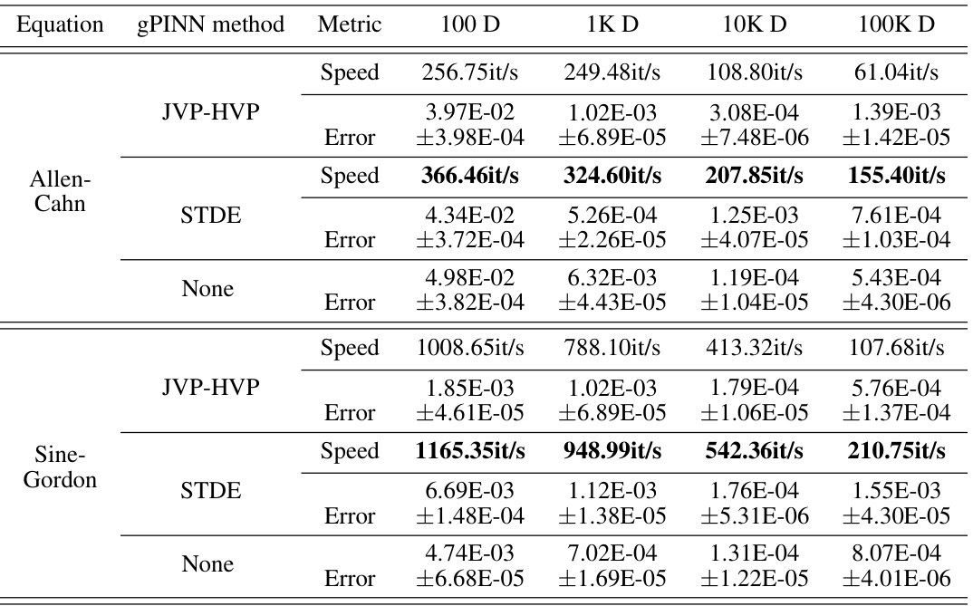
This table presents a comparison of different methods for solving the Inseparable Allen-Cahn equation using PINNs. The methods compared include various versions of SDGD (with and without parallelization and using PyTorch or JAX) and the proposed STDE method. The table shows the speed (iterations per second), memory usage, and error (L2 relative error) for each method at different input dimensions (100D, 1K D, 10K D, 100K D, 1M D). The results demonstrate that STDE significantly outperforms the baseline SDGD methods in terms of both speed and memory efficiency, while maintaining comparable accuracy. The effect of using a smaller batch size for STDE is also shown.
This table presents a comparison of different methods for solving the Inseparable Allen-Cahn equation, focusing on computational speed, memory usage, and error rate. The methods compared include backward mode SDGD (using both PyTorch and JAX), parallelized backward mode SDGD, forward-over-backward SDGD, forward Laplacian, and STDE (with and without a smaller batch size). The results are shown for various input dimensions (100D, 1K D, 10K D, 100K D, and 1M D), demonstrating the performance scaling of each method with increasing dimensionality. The table highlights STDE’s superior performance in terms of speed and memory efficiency, especially in higher dimensions, while maintaining accuracy comparable to other methods.

This table presents the speed (iterations per second) achieved by different methods (backward mode AD, STDE, and STDE*) for training three different PDEs (2D KdV, 2D KP, and 1D g-KdV) with varying network sizes. The ‘Base’ column shows the speed for the base network (L=4, h=128). The other columns show speedups when increasing network depth (L) and width (h). STDE* represents an alternative approach to STDE using lower-order pushforwards. The table demonstrates the speed advantage of STDE and STDE* over standard backward mode AD, particularly as network complexity increases.
This table presents a comparison of different methods for solving the Inseparable Allen-Cahn equation using PINNs. The methods compared include backward mode SDGD (both in PyTorch and JAX implementations), parallelized backward mode SDGD, forward-over-backward SDGD, forward Laplacian, and STDE (with and without a reduced batch size). For each method, the table shows the speed (iterations per second), memory usage, and the L2 relative error for various input dimensions (100D, 1K D, 10K D, 100K D, and 1M D). The results highlight the performance improvements achieved by STDE, particularly in terms of speed and memory efficiency as the dimensionality of the problem increases. The error bars represent standard deviation.
Full paper#
