↗ OpenReview ↗ NeurIPS Proc. ↗ Chat
TL;DR#
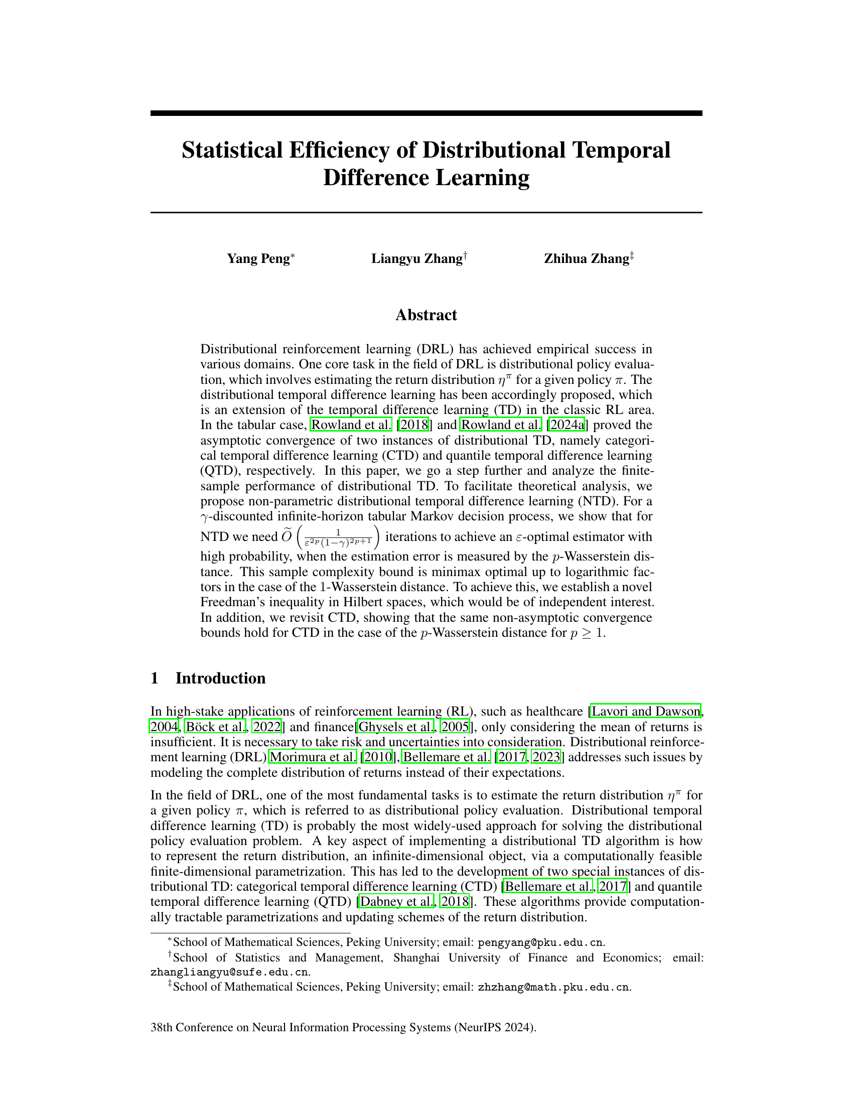
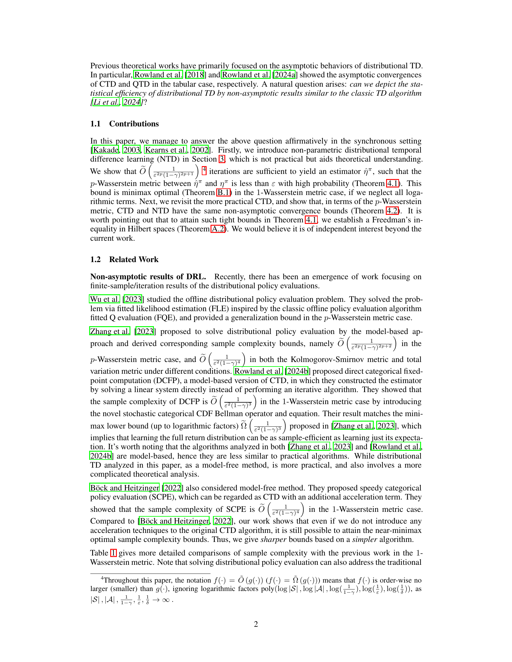
Distributional reinforcement learning (DRL) aims to model the entire distribution of rewards, not just the average, offering a more nuanced approach to decision-making. However, understanding the sample efficiency of DRL algorithms, particularly distributional temporal difference learning (distributional TD), has been limited by a focus on asymptotic analysis. This paper tackles this challenge by providing finite-sample performance analysis which has been lacking.
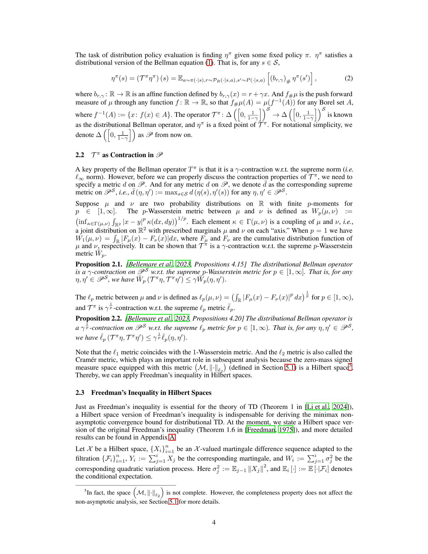
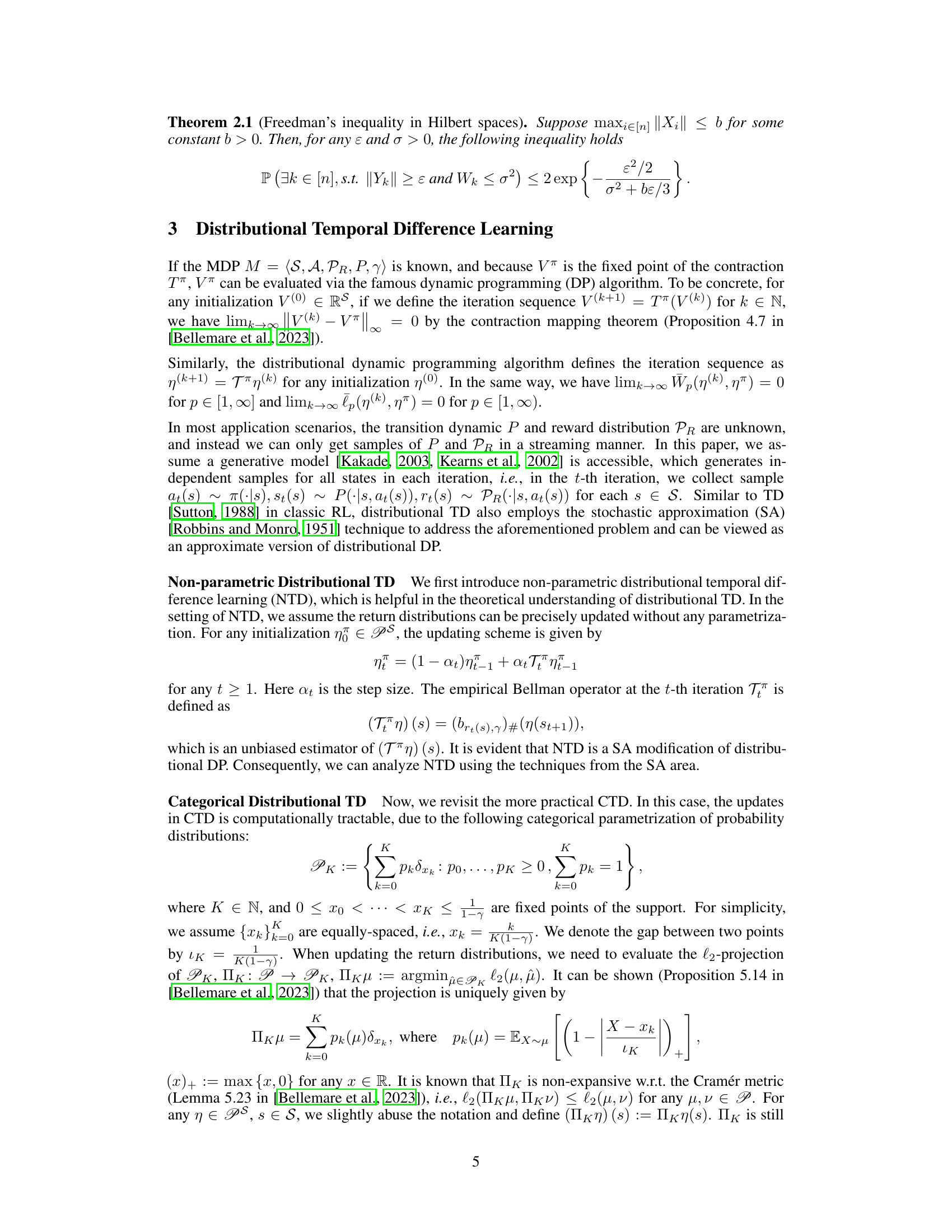
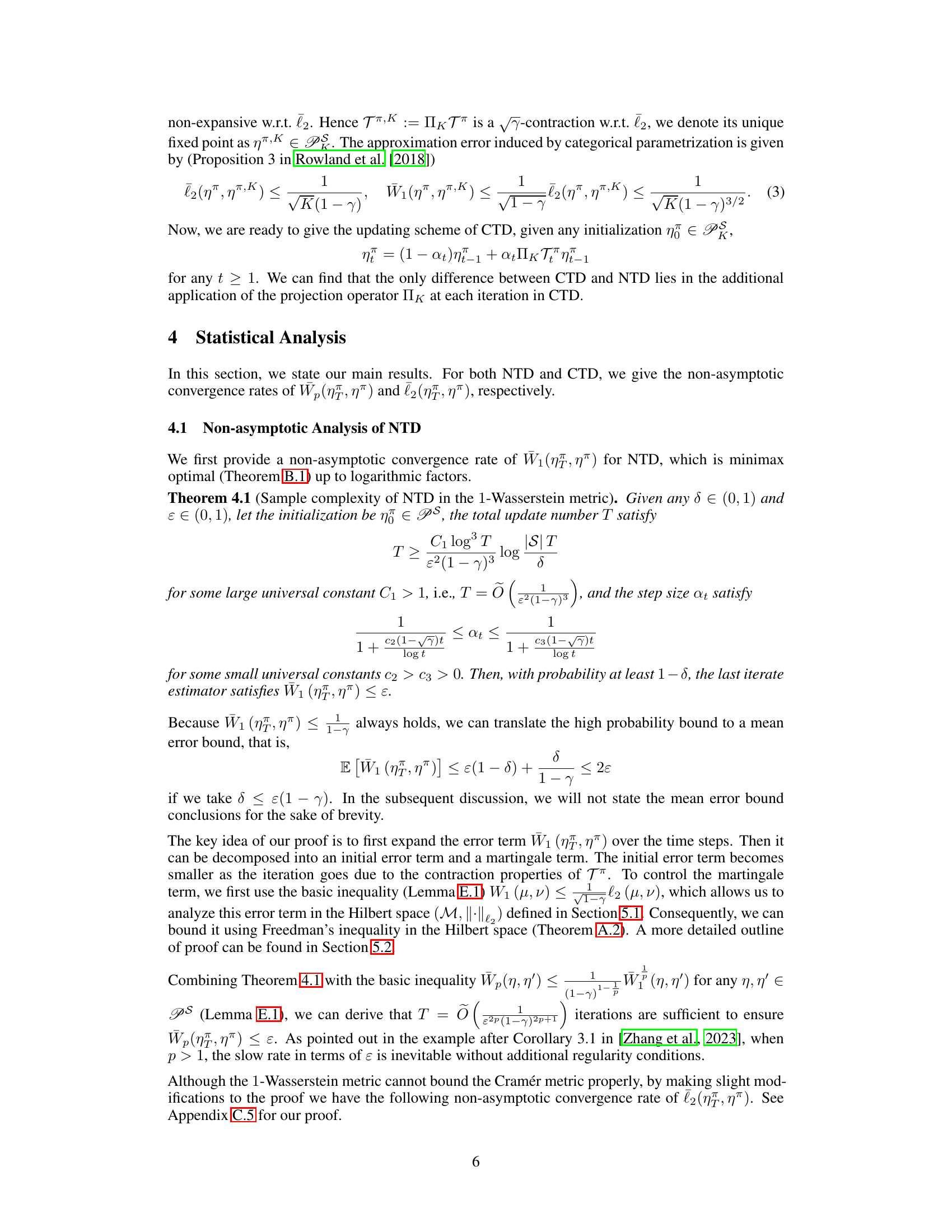
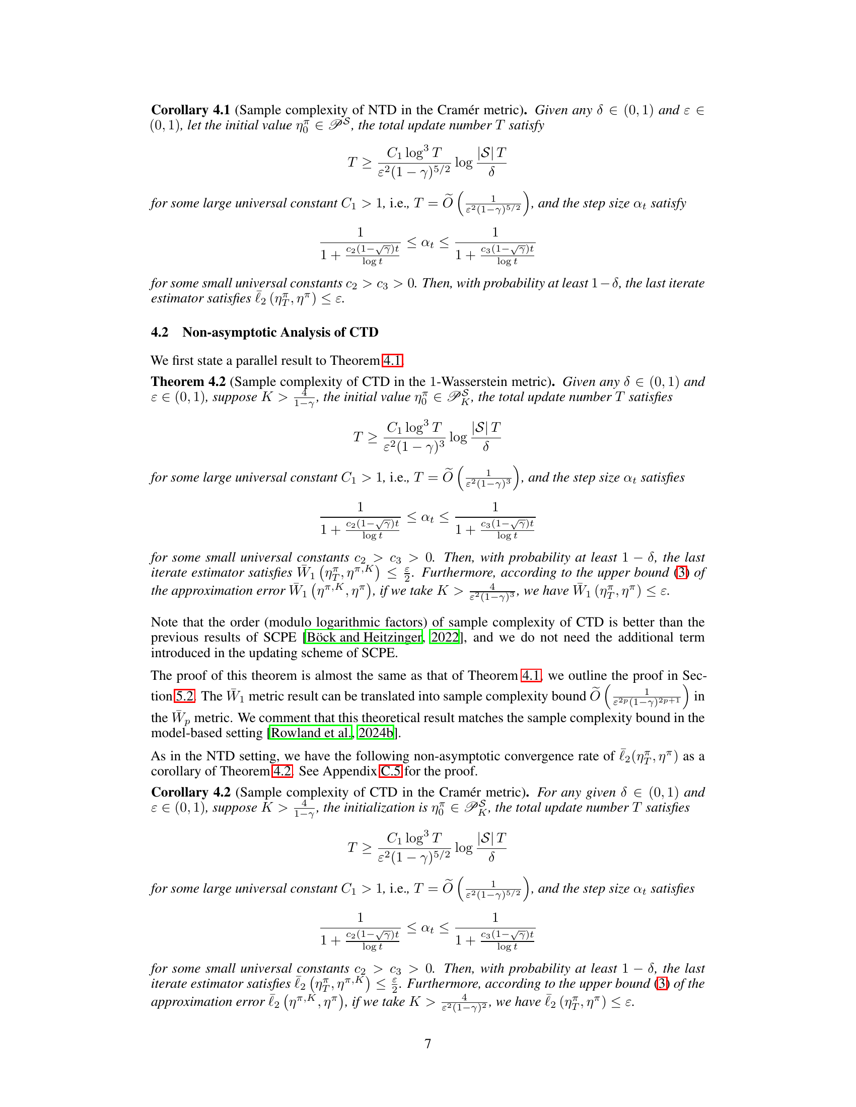
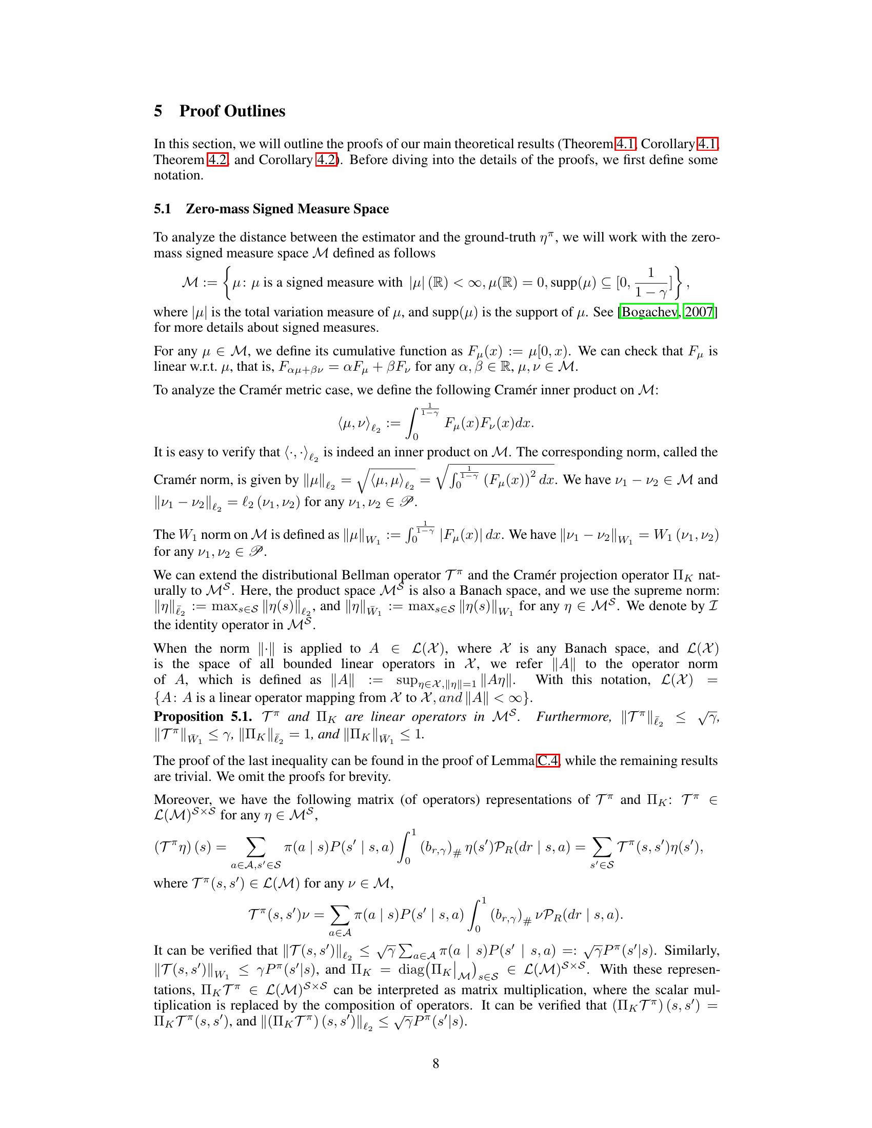
The researchers address this by introducing a novel non-parametric distributional TD, facilitating theoretical analysis. They prove minimax optimal sample complexity bounds under the 1-Wasserstein metric. Importantly, these bounds also apply to the practical categorical TD, showing that tight bounds are achievable without computationally expensive enhancements. Their work is further strengthened by establishing a novel Freedman’s inequality in Hilbert spaces, a result of independent interest beyond the context of DRL.
Key Takeaways#
Why does it matter?#
This paper is crucial for researchers in reinforcement learning as it provides minimax optimal sample complexity bounds for distributional temporal difference learning. This bridges the gap between theory and practice, guiding the development of more efficient algorithms. The novel Freedman’s inequality in Hilbert spaces is also a significant contribution to the broader field of machine learning.
Visual Insights#
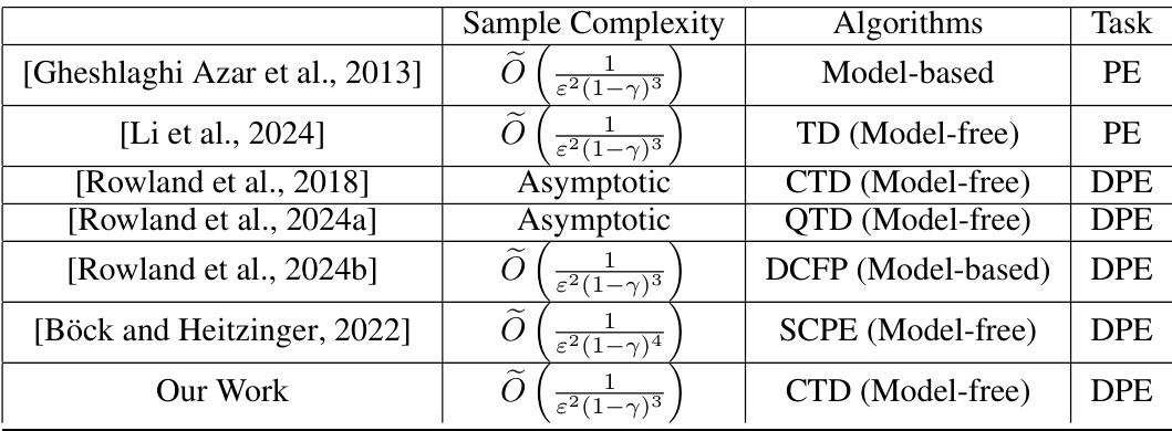
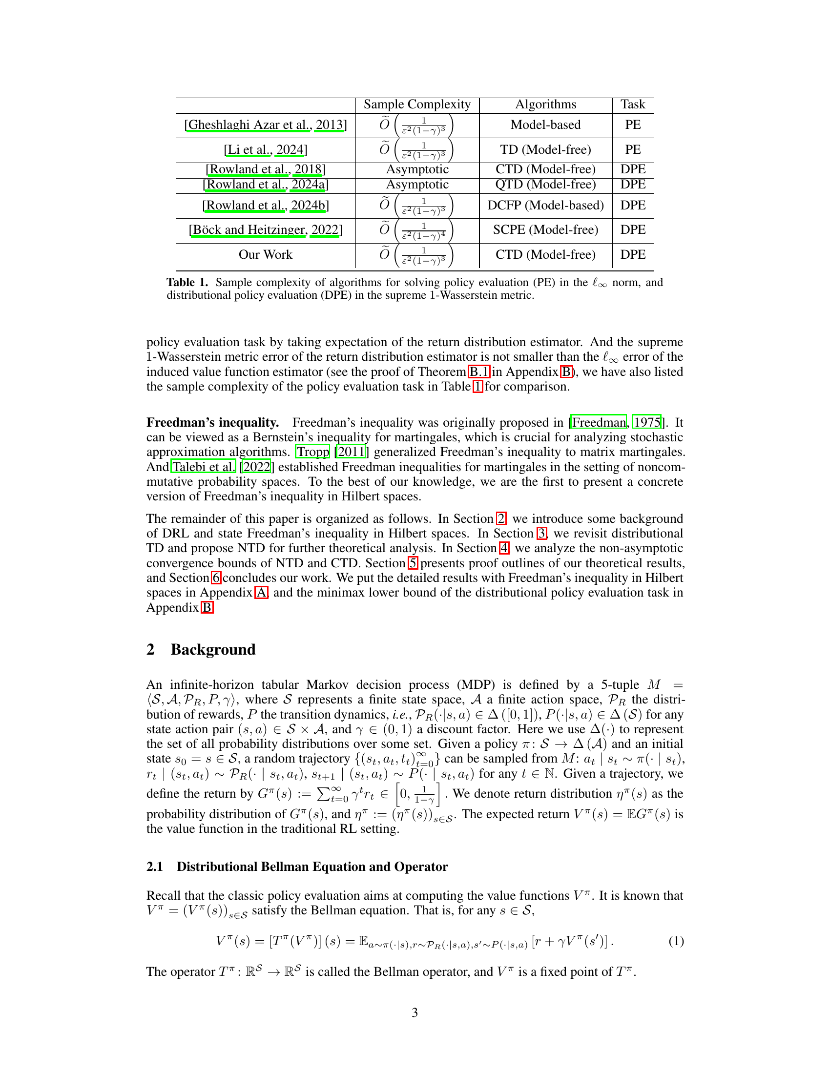
This table compares the sample complexity for solving policy evaluation and distributional policy evaluation problems using different algorithms. The sample complexity is given in terms of the error bound (ε) and the discount factor (γ). Model-based methods typically have lower sample complexity compared to model-free methods. The table shows that our work achieves a near-minimax optimal sample complexity.
Full paper#
