Testing Calibration in Nearly-Linear Time

↗ arXiv ↗ Hugging Face

TL;DR

#

Key Takeaways

#

Why does it matter?

#

This paper is crucial because it tackles the computationally expensive challenge of evaluating model calibration, a critical aspect of machine learning and decision-making. By introducing efficient algorithms, it enables researchers to assess calibration more effectively in large-scale applications and opens new avenues for studying the theoretical aspects of calibration testing.

Visual Insights

#

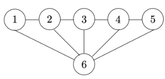
🔼 This figure is a graph with 6 vertices and 9 edges. Vertices 1 through 5 are connected in a line, and each of these vertices is connected to vertex 6. This graph structure is used to reformulate a linear program related to the smooth calibration error (smCE) as a minimum-cost flow problem. This reformulation is crucial to the development of a fast algorithm for calibration testing.

read the caption

Figure 1: Example graph G for n = 5 with n + 1 = 6 vertices and 2n − 1 = 9 edges.

🔼 This table shows the smallest calibration threshold (epsilon) at which the calibration testers (smCE, dCE, ConvECE) correctly identify the calibrated distribution in at least half of the 100 experimental runs. The column index n represents the number of samples used in the experiments. The ground truth calibration error is 0.01.

read the caption

Table 1: Calibration testing thresholds (smallest passed on half of 100 runs).

In-depth insights

#

Calibration Testing

#

Calibration testing, a crucial aspect of evaluating probabilistic prediction models, focuses on assessing whether a model’s predicted probabilities accurately reflect the true likelihood of an event. The core challenge lies in efficiently distinguishing between well-calibrated models and those that are significantly miscalibrated. Traditional methods often rely on binning, but this approach suffers from increased complexity and sensitivity to parameter choices. The paper proposes a novel framework for calibration testing using property testing, offering a more robust and theoretically grounded approach. By leveraging insights from the smooth calibration error, which approximates the lower distance to calibration, the authors design an algorithm that achieves nearly-linear time complexity, providing significant improvements over existing linear programming solutions. Further contributions include analyzing tolerant variants of the problem and establishing sample complexity lower bounds for alternative calibration measures, ultimately demonstrating the effectiveness and efficiency of their proposed framework.

Algorithmic Advances

#

This research significantly advances calibration testing algorithms. A novel, nearly-linear time algorithm for calibration testing is presented, improving upon existing methods with quadratic runtime. This is achieved by reformulating the problem as a minimum-cost flow problem and leveraging a new dynamic programming solver. The work also introduces tolerant variants of the calibration testing problem and provides corresponding algorithms. Furthermore, the paper establishes sample complexity lower bounds for alternative calibration measures, demonstrating the advantages of the proposed approach. The experimental results confirm the practical efficiency and effectiveness of the new algorithms, highlighting significant improvements over existing linear programming solvers. Overall, the paper makes substantial contributions to the algorithmic understanding and practical application of calibration testing in machine learning.

Empirical Evaluation

#

An Empirical Evaluation section in a research paper would ideally present a robust and detailed examination of the proposed methods. It should begin by clearly defining the metrics used to evaluate performance, justifying their selection and appropriateness for the task. A strong emphasis should be placed on the experimental setup, including a description of the datasets used, how they were preprocessed (if any), the training and testing procedures followed, and the hyperparameters chosen for all algorithms. The results should be presented clearly and concisely, using tables, figures, and statistical measures where appropriate. Error bars or confidence intervals would demonstrate the reliability of the results. The discussion should thoroughly analyze the results, relating them back to the stated goals and hypotheses, noting any unexpected outcomes or limitations of the approach. Importantly, the analysis needs to compare results with existing state-of-the-art methods, showing clear improvement or a compelling justification if this is not possible. The overall goal is to provide convincing evidence for the claims made in the paper, leaving no doubt about the effectiveness of the proposed method in the contexts tested.

Lower Bounds

#

The Lower Bounds section of a research paper would typically explore the theoretical limitations of a problem or algorithm. It aims to establish provable limits on what is achievable, often demonstrating that no algorithm can perform better than a certain threshold, regardless of its design. This is crucial because it provides a benchmark against which to evaluate existing algorithms and to guide the development of future ones. In the context of calibration testing, for example, lower bounds would show the minimum number of samples needed to reliably distinguish between a calibrated model and one that is far from calibrated, given a certain error tolerance. These bounds inform the sample complexity of the problem, highlighting the inherent difficulty of achieving high accuracy and showing the fundamental limits imposed by statistical uncertainty. Establishing tight lower bounds requires sophisticated techniques and often involves constructing adversarial examples or using information-theoretic arguments to prove that no algorithm can achieve better performance. Tight lower bounds would offer a strong theoretical guarantee on the optimality (or near-optimality) of developed algorithms and highlight potential avenues for future research.

Future Work

#

Future research directions stemming from this work could explore extending the calibration testing framework to more complex prediction settings, such as multi-class classification and regression. Investigating the impact of different calibration measures and their associated sample complexities on the effectiveness of testing would be valuable. Furthermore, developing more efficient algorithms for computing and approximating calibration measures is a crucial area for future work, especially for large datasets. The development of novel calibration measures that are both statistically sound and computationally tractable warrants further investigation. Exploring the theoretical limits of calibration testing and determining the necessary sample complexity for achieving desired accuracy levels are important open problems. Finally, applying these calibration testing techniques to real-world applications, evaluating their impact, and developing practical tools for assessing calibration in industrial settings would significantly contribute to the broader machine learning community.

More visual insights

#

More on figures

🔼 This figure compares the performance of three different calibration error measures (smCE, dCE, and ConvECE) in detecting miscalibration in synthetic datasets. The x-axis represents the dataset size (2^x+1), and the y-axis represents the median error of the three methods, with error bars showing the 25th and 75th percentiles across 100 runs. The results demonstrate that smCE and dCE are more reliable in estimating the true calibration error than ConvECE, especially as the sample size increases.

read the caption

Figure 2: The 25% quantile, median, and 75% quantile (over 100 runs) for smCE, dCE and CECE respectively. The x-axis is for dataset with size 2^x + 1.

🔼 This figure is a graph showing an example of the graph structure used in the dynamic programming algorithm to solve the smooth calibration linear program in the paper. It has 6 vertices and 9 edges. The structure is designed to efficiently represent the constraints in the linear program, making the problem amenable to a dynamic programming solution. The vertices represent the variables, and the edges represent relationships between these variables (constraints). The graph’s particular arrangement allows for an efficient algorithm to compute the minimum-cost flow, which corresponds to the solution of the linear program.

read the caption

Figure 1: Example graph G for n = 5 with n + 1 = 6 vertices and 2n − 1 = 9 edges.

More on tables

🔼 This table presents the empirical smooth calibration error (smCE) for three different distributions obtained by post-processing the predictions of a DenseNet40 model trained on the CIFAR-100 dataset. The three distributions are: Dbase (original model predictions), Diso (predictions after isotonic regression), and Dtemp (predictions after temperature scaling). The median smCE across 20 runs is reported for each distribution. The results show that temperature scaling leads to lower smooth calibration error than the original model and isotonic regression.

read the caption

Table 2: Empirical smCE on postprocessed DenseNet40 predictions (median over 20 runs)

🔼 This table compares the runtime performance of four different solvers for computing the value of equation (3) in the paper, which is a linear program representing the smooth calibration error. The solvers compared are CVXPY’s linear program solver, Gurobi’s minimum-cost flow solver, a custom dynamic programming solver from Corollary 1 in the paper, and the custom solver further optimized with PyPy. The table shows how the runtime of each solver scales with increasing sample size (n), demonstrating the efficiency gains achieved by the custom dynamic programming solver, especially when combined with PyPy.

read the caption

Table 3: Runtimes (in seconds) for computing the value of (3), using various solvers

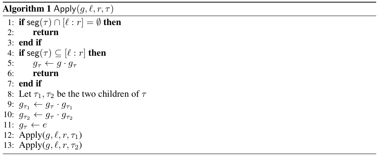
🔼 This table presents the results of calibration testing experiments using three different calibration measures: smCE, dCE, and ConvECE. The goal was to determine the smallest threshold epsilon for each measure that correctly identifies a miscalibrated distribution (i.e., a distribution with non-zero distance to calibration) in at least half of 100 trials. The number of samples (n) was varied, and the ground truth distance to calibration (0.01) is also shown. The results indicate the relative performance of these calibration measures for calibration testing, highlighting the reliability of smCE and dCE compared to ConvECE.

read the caption

Table 1: Calibration testing thresholds (smallest passed on half of 100 runs).

🔼 This table presents the results of calibration testing experiments using three different calibration measures: smooth calibration error (smCE), lower distance to calibration (dCE), and convolved ECE (ConvECE). For various sample sizes (n), the table shows the smallest threshold (ε) such that a majority of 100 runs of an ε-tester reported ‘yes’, indicating that the distribution is calibrated. This is compared to the ground truth calibration error of 0.01. The table demonstrates that smCE and dCE testers are more reliable estimators of the ground truth calibration error than ConvECE.

read the caption

Table 1: Calibration testing thresholds (smallest passed on half of 100 runs).

Full paper

#