TL;DR#
Many machine learning applications rely on sparse models, which require identifying a small subset of the most important features or parameters from a vast dataset. Iterative Hard Thresholding (IHT) is a common method for this task, but it can be computationally expensive, especially for large datasets. This often limits its usage when dealing with big data.
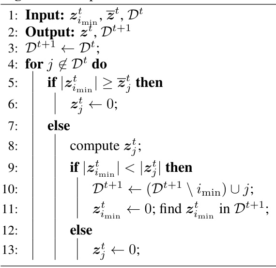
This research introduces a novel method that significantly speeds up IHT. It achieves this by cleverly avoiding unnecessary calculations during the optimization process. The method carefully identifies and ignores parameters that are unlikely to contribute significantly to the final solution. The researchers demonstrate that their improved IHT is up to 73 times faster than the standard IHT, without compromising accuracy. Crucially, the new method doesn’t require manual tuning of hyperparameters, making it more user-friendly and efficient.
Key Takeaways#
Why does it matter?#
This paper is crucial for researchers working on sparse optimization and high-dimensional data analysis. It offers a significant speedup for a widely used method, impacting various fields that rely on sparse models. The safe pruning strategy is particularly valuable, ensuring accuracy is not compromised, while the automatic hyperparameter determination simplifies application and broadens accessibility. Further research could explore extending the method to other optimization problems or incorporating different sparsity-inducing penalties.
Visual Insights#
🔼 This figure compares the performance of the proposed FastIHT method against three other methods (IHT, RegIHT, and AccIHT) across five datasets and various values of k (sparsity level). Subfigures (a) through (e) show the log processing times for each dataset. Subfigure (f) shows the number of gradient computations for the gisette dataset, highlighting the significant reduction achieved by FastIHT. Subfigure (g) demonstrates the performance of FastIHT with a larger step size on the gisette dataset.
read the caption
Figure 1: (a)-(e): Comparisons of log processing times for each dataset and k. (f): Comparison of number of gradient computations on gisette. (g): Comparisons of log processing times for gisette with a large step size. Some results of AccIHT are omitted since they could not converge.

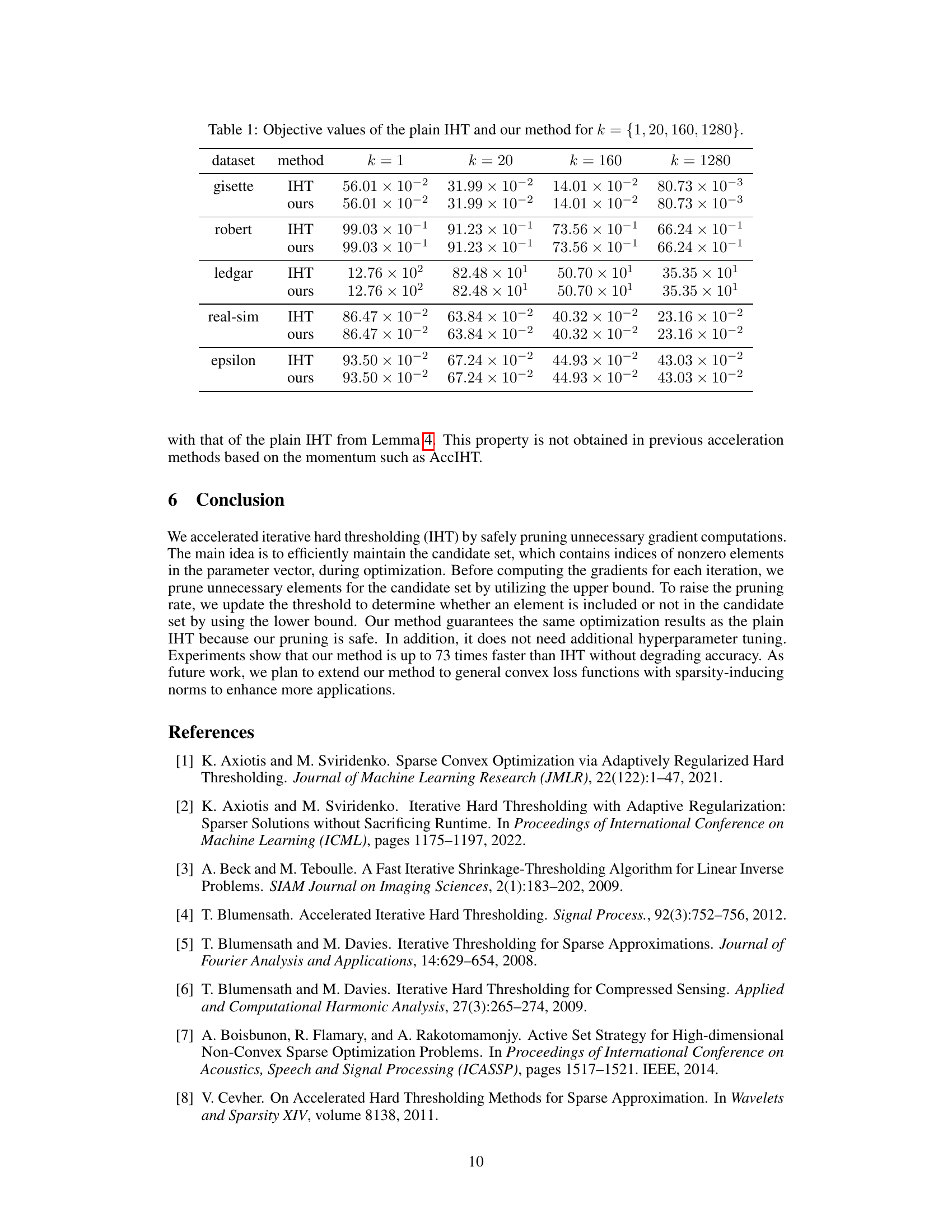
🔼 This table compares the objective values achieved by the plain IHT and the proposed Fast IHT method for different sparsity levels (k). The results demonstrate that both methods achieve the same objective values, confirming the theoretical guarantee that the proposed method does not compromise accuracy while significantly reducing computation time.
read the caption
Table 1: Objective values of the plain IHT and our method for k ∈ {1, 20, 160, 1280}
In-depth insights#
IHT Acceleration#
IHT acceleration techniques significantly improve the efficiency of sparse parameter recovery in linear regression. Traditional IHT’s main computational bottleneck is gradient calculation. Methods focusing on IHT acceleration often target this step. Pruning strategies, such as those explored in the provided research, identify and eliminate unnecessary gradient computations by leveraging upper and lower bounds on parameter values. This selectively updates only the most promising parameters, significantly reducing processing time. Other approaches incorporate momentum techniques from other optimization algorithms, accelerating convergence towards the sparse solution and thus reducing the number of iterations needed. The success of IHT acceleration hinges on a careful balance between computational savings and the accuracy of the final sparse vector. While aggressive pruning can dramatically reduce time, it may compromise solution quality. Therefore, sophisticated strategies often employ adaptive methods to adjust pruning intensity or momentum strength based on the optimization progress. The overall goal is to achieve a substantial speedup without compromising the crucial sparsity or accuracy properties of the IHT algorithm.
Gradient Pruning#
Gradient pruning is a technique aimed at accelerating gradient-based optimization algorithms by selectively reducing the number of gradient computations. The core idea is to identify and disregard gradients that are deemed insignificant or redundant to the overall optimization process. This can significantly reduce the computational cost, especially for high-dimensional problems. Effective gradient pruning strategies often employ heuristics or approximations to estimate gradient significance without explicitly calculating all gradients. This involves balancing the trade-off between computational savings and the potential loss of accuracy resulting from omitting gradients. Successful gradient pruning techniques usually incorporate mechanisms for dynamically adapting pruning criteria based on the optimization progress. This adaptive approach helps to avoid premature or excessive pruning that might hinder convergence. Ultimately, the effectiveness of gradient pruning depends on the specific algorithm, the problem’s characteristics, and the sophistication of the pruning strategy.
Candidate Set#
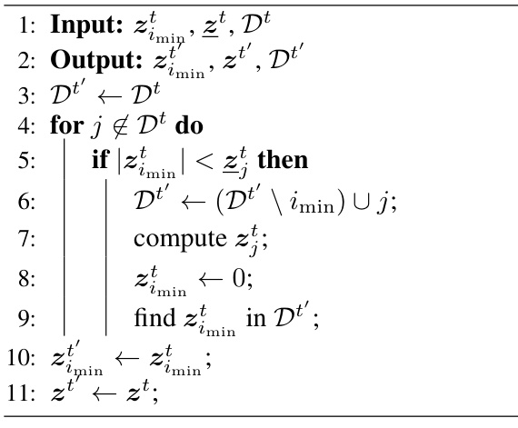
The concept of a ‘Candidate Set’ in the context of sparse optimization algorithms, like the Iterative Hard Thresholding (IHT) method discussed in the paper, is crucial for efficiency. It represents a carefully selected subset of the parameter vector’s indices, containing only those elements likely to be non-zero in the final solution. Constructing this set efficiently is key, as it allows the algorithm to focus computations on the most promising elements, significantly reducing the processing time. The paper’s approach to constructing the candidate set involves using upper and lower bounds on the absolute values of parameters, allowing for the safe pruning of unnecessary gradient computations. This clever technique ensures that the final solution is not compromised while gaining significant computational speedups. The efficiency of the candidate set’s construction and its role in pruning gradient computations are central to the paper’s claim of a substantially faster IHT method.
Upper/Lower Bounds#
The concept of upper and lower bounds is crucial for the algorithm’s efficiency. Upper bounds on the absolute values of parameters allow for the safe pruning of gradient computations. By establishing that a parameter’s upper bound is below a certain threshold, the algorithm avoids calculating gradients for that parameter, significantly speeding up the process. Conversely, lower bounds play a vital role in determining this threshold dynamically. The algorithm leverages the lower bound to ensure that it only prunes computations for parameters that are genuinely unimportant for the current iteration. The interplay between these bounds is key: the upper bound enables the pruning, while the lower bound safeguards against premature or inaccurate pruning. The effectiveness of this method hinges on the tightness of these bounds—tighter bounds lead to more efficient pruning without sacrificing accuracy. The dynamic adjustment of the threshold, based on the interplay of upper and lower bounds, is a key innovation that allows for an adaptive pruning strategy optimized for each iteration.
Future Work#
The “Future Work” section of this research paper on accelerating iterative hard thresholding (IHT) would logically focus on extending the algorithm’s capabilities and addressing limitations. A crucial direction would be to generalize the pruning strategy to handle other convex loss functions and sparsity-inducing norms, moving beyond the linear regression model with the l0-norm constraint. This would significantly broaden the algorithm’s applicability to a wider range of machine learning problems. Another important area is to investigate the theoretical properties of the algorithm with non-convex loss functions, potentially developing convergence guarantees under certain conditions. Further exploration into the optimal selection of the step size and threshold parameters, perhaps using adaptive methods or learning techniques, could improve the algorithm’s efficiency and robustness. Finally, thorough empirical evaluations on diverse datasets are needed to demonstrate the effectiveness and scalability of the generalized algorithm across various problem settings. Investigating the practical trade-offs between pruning efficiency and convergence rate for different dataset characteristics would be particularly insightful. Lastly, exploring the algorithm’s performance with very large-scale datasets (using distributed computing techniques) is a highly practical aspect meriting further research.
More visual insights#
More on figures
🔼 This figure compares the performance of the proposed FastIHT method against several baselines (IHT, RegIHT, and AccIHT) across five datasets (gisette, robert, ledgar, real-sim, and epsilon) and various values of k (sparsity level). Subfigures (a) through (e) show log processing times for each dataset, demonstrating that FastIHT is significantly faster. Subfigure (f) specifically illustrates the substantial reduction in the number of gradient computations achieved by FastIHT on the gisette dataset. Finally, subfigure (g) shows the consistent speed advantage of FastIHT even when using a larger step size. Note that some results for AccIHT are missing due to failure to converge in those instances.
read the caption
Figure 1: (a)-(e): Comparisons of log processing times for each dataset and k. (f): Comparison of number of gradient computations on gisette. (g): Comparisons of log processing times for gisette with a large step size. Some results of AccIHT are omitted since they could not converge.
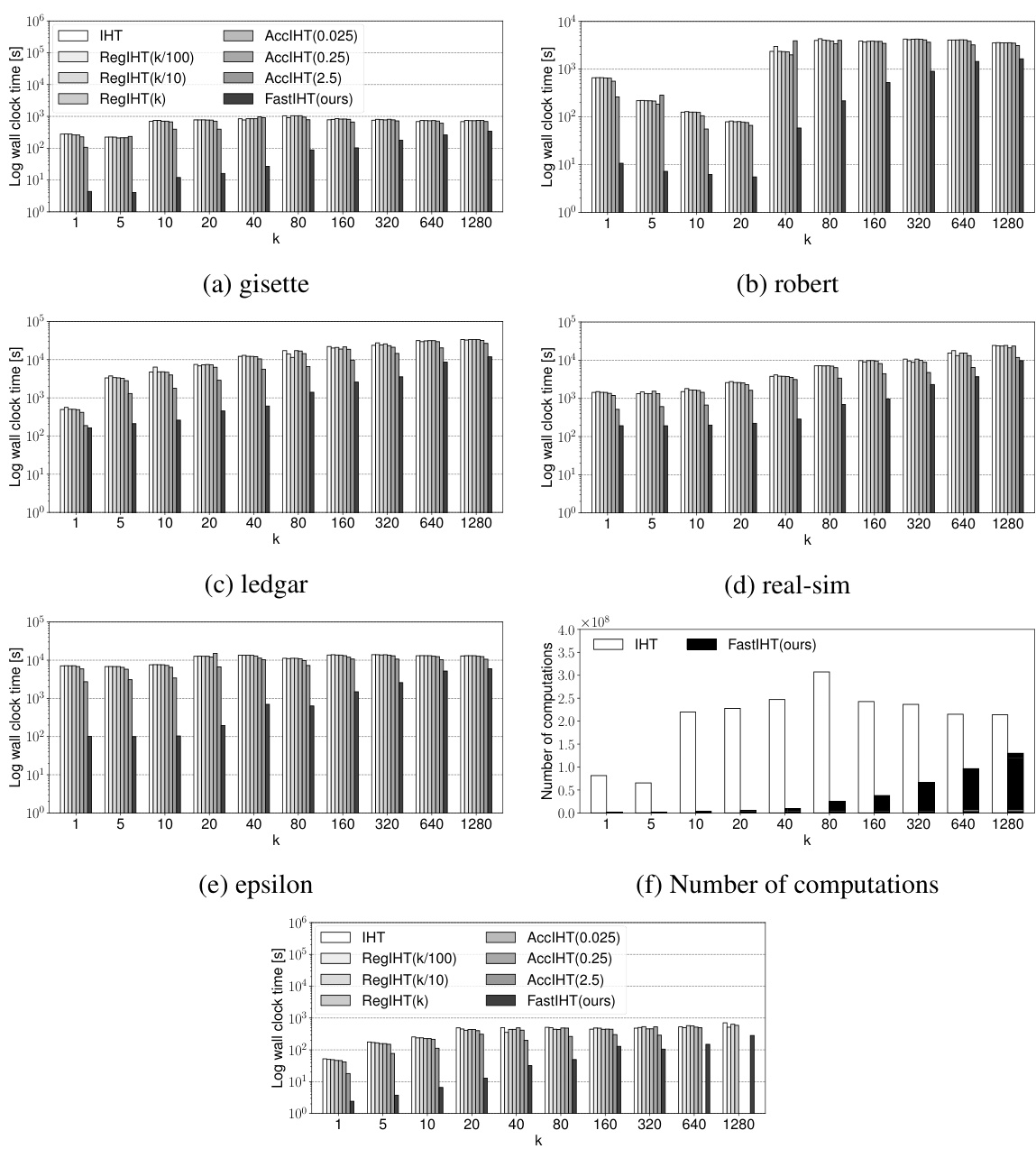
🔼 This figure compares the performance of different algorithms for feature selection tasks. Subfigures (a) through (e) show the log processing time of five datasets (gisette, robert, ledgar, real-sim, and epsilon) for different values of k (the number of selected features). Subfigure (f) shows the number of gradient computations required by the proposed method (FastIHT) and plain IHT for the gisette dataset. Subfigure (g) shows log processing times for the gisette dataset when the step size is increased. The results show that the proposed method is significantly faster than existing methods for all datasets and k values, and its performance is robust even with a larger step size.
read the caption
Figure 1: (a)-(e): Comparisons of log processing times for each dataset and k. (f): Comparison of number of gradient computations on gisette. (g): Comparisons of log processing times for gisette with a large step size. Some results of AccIHT are omitted since they could not converge.
More on tables
🔼 This table presents a comparison of objective values achieved by the plain IHT and the proposed fast IHT method for different sparsity levels (k). The objective function is the mean squared error in the linear regression model. The results demonstrate that both methods achieve practically identical objective values across various datasets and sparsity levels, thereby validating the claim that the proposed method maintains accuracy while improving speed.
read the caption
Table 1: Objective values of the plain IHT and our method for k ∈ {1, 20, 160, 1280}
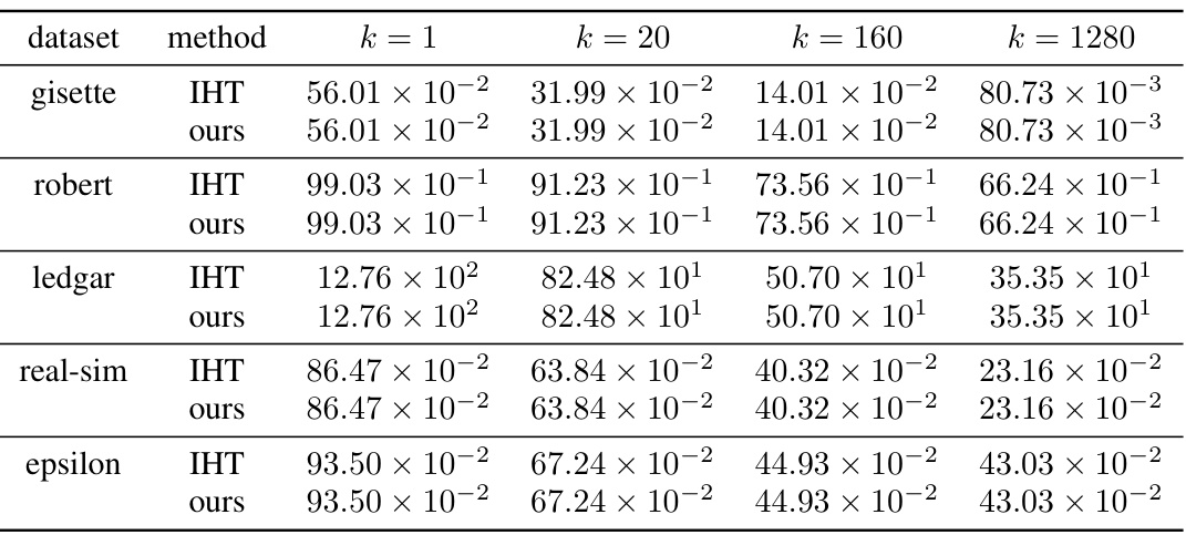
🔼 This table presents a comparison of objective values obtained using the plain Iterative Hard Thresholding (IHT) method and the proposed fast IHT method for various values of k (the number of non-zero elements in the parameter vector). The results are shown for four different datasets: gisette, robert, ledgar, real-sim, and epsilon. Each row represents a dataset, while the columns represent the objective function values achieved by the plain IHT and the proposed method for different values of k. The table demonstrates that the proposed method achieves the same objective values as the plain IHT, showing its accuracy and effectiveness.
read the caption
Table 1: Objective values of the plain IHT and our method for k ∈ {1, 20, 160, 1280}.
Full paper#
