TL;DR#
Many scientific applications involve estimating the distribution of parameters that best match observed data. This is challenging because many parameter distributions can lead to nearly identical data. Existing methods often struggle with this ill-posedness, and those that use likelihood-based approaches are not applicable to simulators with intractable likelihoods.
This paper introduces Sourcerer, a new method that uses the maximum entropy principle. Sourcerer works directly from samples generated from the simulator and doesn’t require computing likelihoods, overcoming the limitations of existing approaches. Sourcerer successfully recovers source distributions with significantly higher entropy without compromising simulation accuracy across various benchmark tasks, including a real-world electrophysiology dataset.
Key Takeaways#
Why does it matter?#
This paper is crucial for researchers working with complex simulators, especially those with intractable likelihoods. It offers a principled method for inferring source distributions, maximizing entropy to retain uncertainty while ensuring simulation fidelity. This is highly relevant to various scientific fields, opening avenues for enhanced inference and model exploration.
Visual Insights#
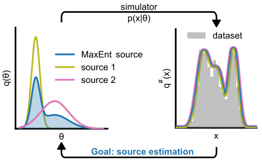
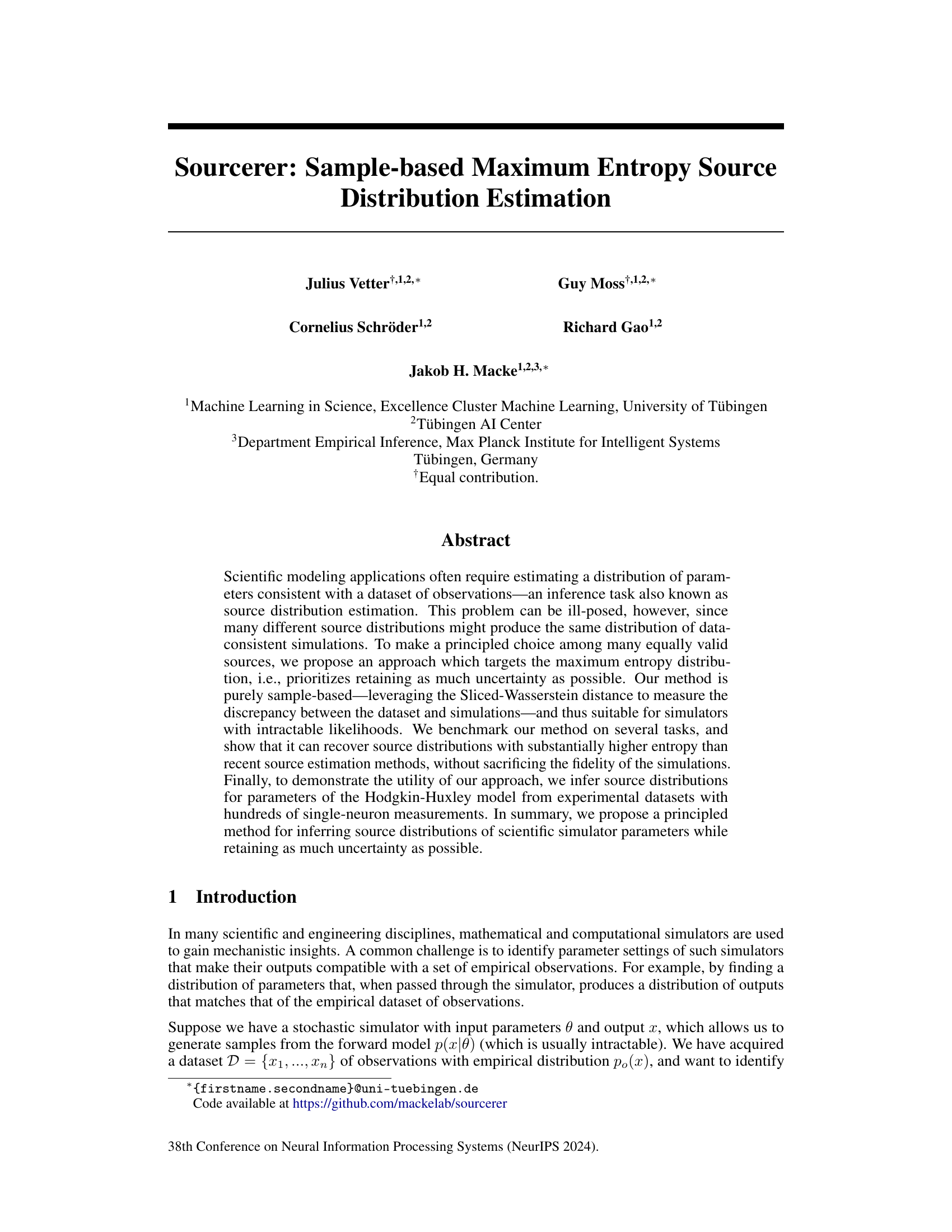
🔼 The figure illustrates the concept of maximum entropy source distribution estimation. It shows that multiple different source distributions q(θ) can produce the same data distribution q#(x) after being passed through a simulator p(x|θ). This is a problem because the inference task (source distribution estimation) becomes ill-posed; there isn’t a unique solution. The solution proposed in the paper is to select the maximum entropy source distribution, which is guaranteed to be unique.
read the caption
Figure 1: Maximum entropy source distribution estimation. Given an observed dataset D = {x1,...,xn} from some data distribution p₀(x), the source distribution estimation problem is to find the parameter distribution q(θ) that reproduces p₀(x) when passed through the simulator p(x|θ), i.e. q#(x) = ∫ p(x|θ)q(θ)dθ = p(x) for all x. This problem can be ill-posed, as there might be more than one distinct source distribution. We resolve this by targeting the maximum entropy distribution, which is unique.
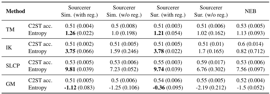
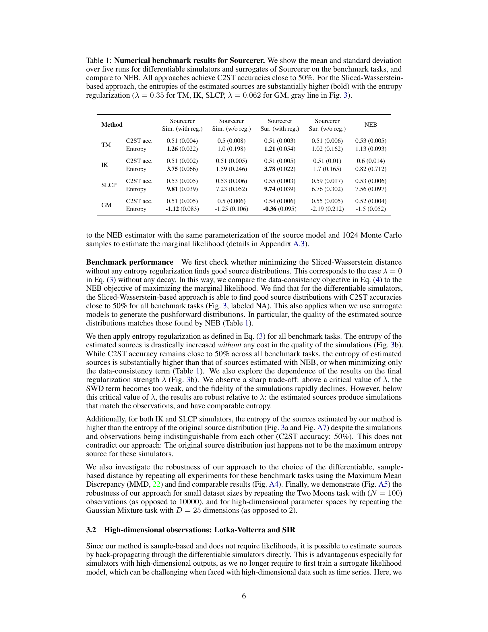
🔼 This table presents a quantitative comparison of the proposed Sourcerer method against a state-of-the-art approach (NEB) for source distribution estimation. The comparison is performed across four benchmark tasks, using both original differentiable simulators and learned surrogates. The table shows the mean and standard deviation of C2ST accuracy (a measure of how well the estimated source distribution reproduces the observed data distribution) and the entropy of the estimated source distributions over five independent runs. The results highlight Sourcerer’s ability to achieve high entropy without sacrificing accuracy, especially when using entropy regularization.
read the caption
Table 1: Numerical benchmark results for Sourcerer. We show the mean and standard deviation over five runs for differentiable simulators and surrogates of Sourcerer on the benchmark tasks, and compare to NEB. All approaches achieve C2ST accuracies close to 50%. For the Sliced-Wasserstein-based approach, the entropies of the estimated sources are substantially higher (bold) with the entropy regularization (λ = 0.35 for TM, IK, SLCP, λ = 0.062 for GM, gray line in Fig. 3).
In-depth insights#
MaxEnt Source Estimation#
MaxEnt source estimation presents a novel approach to a long-standing challenge in scientific modeling: inferring the underlying distribution of simulator parameters from observational data. The method leverages the principle of maximum entropy, prioritizing the most uncertain distribution that’s still consistent with the data. This elegantly addresses the ill-posed nature of the problem, where multiple parameter distributions could lead to similar observations. The use of the Sliced-Wasserstein distance further enhances the approach’s practicality by enabling evaluation without relying on tractable likelihood functions, which are often unavailable for complex scientific simulators. This sample-based approach makes MaxEnt source estimation broadly applicable, demonstrating superior performance in recovering high-entropy distributions across various tasks, from simple benchmarks to complex real-world datasets. The combination of maximum entropy and the Sliced-Wasserstein distance marks a significant contribution, offering a robust and principled method for navigating the inherent uncertainties in scientific model inference.
Sample-Based Inference#
Sample-based inference, as a methodology, offers a compelling alternative to traditional likelihood-based approaches, particularly when dealing with complex or intractable models. Its strength lies in its ability to work directly with simulated data, bypassing the need for explicit likelihood calculations. This is crucial for many scientific applications where models are highly complex and the likelihood function is either unavailable or computationally expensive to evaluate. By focusing on the distance between simulated and observed data distributions, sample-based methods offer a flexible and powerful framework. The choice of distance metric is key and must be carefully considered to match the problem’s unique features. The Sliced Wasserstein Distance (SWD) is highlighted in the paper for its computational efficiency and differentiability. However, the generalizability of the approach depends on the choice of distance metric and its suitability for high-dimensional data. The maximum entropy principle, as adopted by the authors, provides a principled approach for choosing among equally valid solutions, which is especially beneficial in cases where the inverse problem is ill-posed. By maximizing entropy, the method effectively incorporates uncertainty quantification into the estimation procedure, which is a significant advantage for scientific modeling. The method’s sample-based nature enables its application to scientific simulators with complex dynamics, potentially opening up new avenues for analyzing complex scientific systems where likelihood-based methods fall short. The demonstrated applications to electrophysiological data analysis and other high-dimensional problems showcases the significant impact of this approach.
Sliced-Wasserstein Metric#
The Sliced-Wasserstein distance is a powerful tool for comparing probability distributions, particularly useful when dealing with high-dimensional data or intractable likelihoods. It cleverly addresses the computational challenges of directly calculating Wasserstein distances in high dimensions by projecting the distributions onto many lower-dimensional subspaces (typically one-dimensional). The Wasserstein distance is then computed on these projections, and the final Sliced-Wasserstein distance is the average of these lower-dimensional distances. This approach offers a significant computational advantage, making it suitable for large datasets and complex simulations. Its differentiability is a key strength, allowing for use in gradient-based optimization methods, as demonstrated in the paper’s source distribution estimation framework. However, the choice of the number of projections and the type of projection can influence results. Careful consideration must be given to the selection of these hyperparameters to ensure robust and reliable comparisons, especially in the presence of complex data structures or significant noise.
High-Dimensional Results#
In the realm of high-dimensional data analysis, the challenges are amplified significantly. This section would likely delve into the application of the proposed maximum entropy method to datasets exhibiting high dimensionality, possibly examining both deterministic and probabilistic simulators. The core focus would be to demonstrate the robustness and scalability of the method when dealing with a large number of variables or parameters, particularly where traditional likelihood-based methods struggle. A key element would be evaluating its performance against established baselines, assessing the fidelity of the resulting simulations, and examining the trade-off between accuracy and the preservation of uncertainty (high entropy) in the inferred source distributions. The use of sample-based metrics, such as the Sliced-Wasserstein distance, is crucial in this setting to bypass the computational limitations of high-dimensional likelihood calculations, and its efficacy would be a central point of discussion. The section would likely present compelling case studies, possibly including specific applications within scientific domains where high-dimensional data is prevalent, showcasing the benefits and practical utility of this novel approach.
Hodgkin-Huxley Model#
The Hodgkin-Huxley model, a cornerstone of neurophysiology, is tackled in this research with a novel approach. The paper uses the model not to simulate neuron behavior directly, but as a complex, high-dimensional simulator within a broader framework of source distribution estimation. This is a significant departure from typical uses of the model, demonstrating its adaptability as a testing ground for advanced statistical methods. Instead of focusing on precise parameter fitting, the study aims to infer a distribution of parameters that, when run through the model, reproduces observed electrophysiological data. The use of this model highlights the power of the proposed maximum-entropy approach, which excels when dealing with ill-posed inverse problems where many parameter sets can yield similar output. The authors leverage the model’s complexity to evaluate their methodology’s robustness, which is noteworthy given the high-dimensionality of the model’s parameter space and the high volume of real-world data used for validation. The results obtained from the Hodgkin-Huxley model showcase the practical application of their source estimation technique, a valuable contribution to the field of scientific inference, where uncertainty quantification is critical.
More visual insights#
More on figures

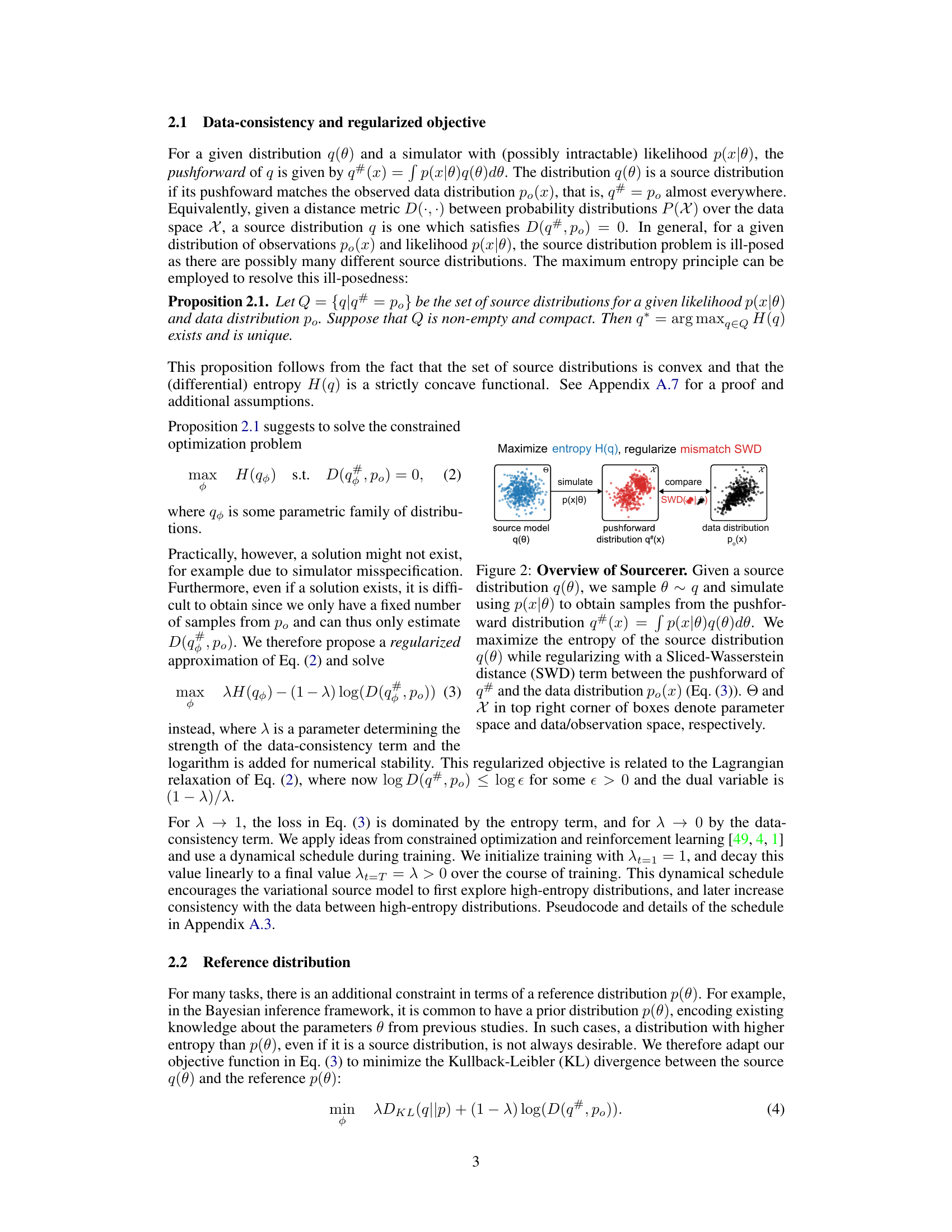
🔼 This figure illustrates the Sourcerer method. It begins with a source model, q(θ), which generates samples of parameters θ. These parameters are then passed through a simulator, p(x|θ), producing samples of simulated data, q#(x). The Sliced-Wasserstein Distance (SWD) measures the discrepancy between the simulated data (q#(x)) and the observed data distribution, p₀(x). The goal is to find the maximum entropy distribution q(θ) that minimizes the SWD, balancing between maximizing entropy (uncertainty) and matching the observed data.
read the caption
Figure 2: Overview of Sourcerer. Given a source distribution q(θ), we sample θ ~ q and simulate using p(x|θ) to obtain samples from the pushforward distribution q#(x) = ∫p(x|θ)q(θ)dθ. We maximize the entropy of the source distribution q(θ) while regularizing with a Sliced-Wasserstein distance (SWD) term between the pushforward of q# and the data distribution p₀(x) (Eq. (3)). θ and x in top right corner of boxes denote parameter space and data/observation space, respectively.

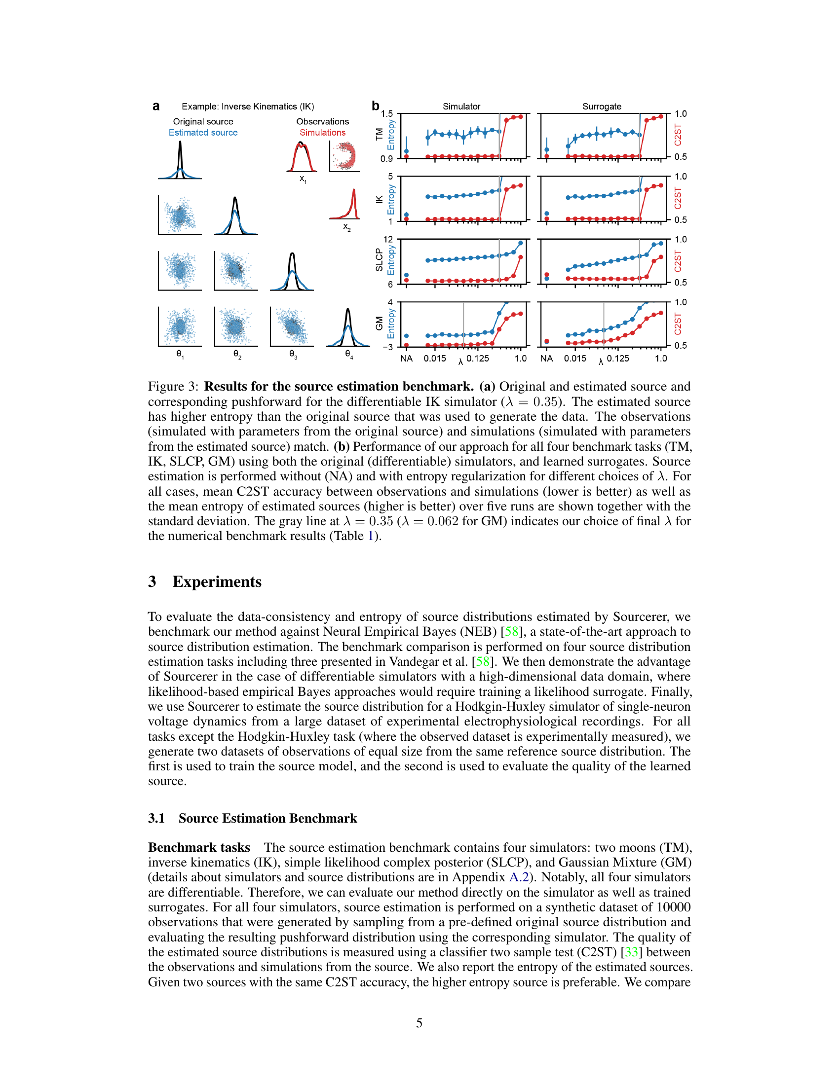
🔼 Figure 3 presents a comparison of the proposed Sourcerer method against a state-of-the-art approach for source distribution estimation. Panel (a) shows an example using a differentiable Inverse Kinematics simulator, illustrating how Sourcerer finds a higher-entropy source distribution that still accurately matches the observed data. Panel (b) presents a quantitative comparison across four benchmark tasks, showing Sourcerer’s superior performance in terms of both accuracy (C2ST) and higher entropy of the estimated sources across different regularization strengths.
read the caption
Figure 3: Results for the source estimation benchmark. (a) Original and estimated source and corresponding pushforward for the differentiable IK simulator (λ = 0.35). The estimated source has higher entropy than the original source that was used to generate the data. The observations (simulated with parameters from the original source) and simulations (simulated with parameters from the estimated source) match. (b) Performance of our approach for all four benchmark tasks (TM, IK, SLCP, GM) using both the original (differentiable) simulators, and learned surrogates. Source estimation is performed without (NA) and with entropy regularization for different choices of λ. For all cases, mean C2ST accuracy between observations and simulations (lower is better) as well as the mean entropy of estimated sources (higher is better) over five runs are shown together with the standard deviation. The gray line at λ = 0.35 (λ = 0.062 for GM) indicates our choice of final λ for the numerical benchmark results (Table 1).

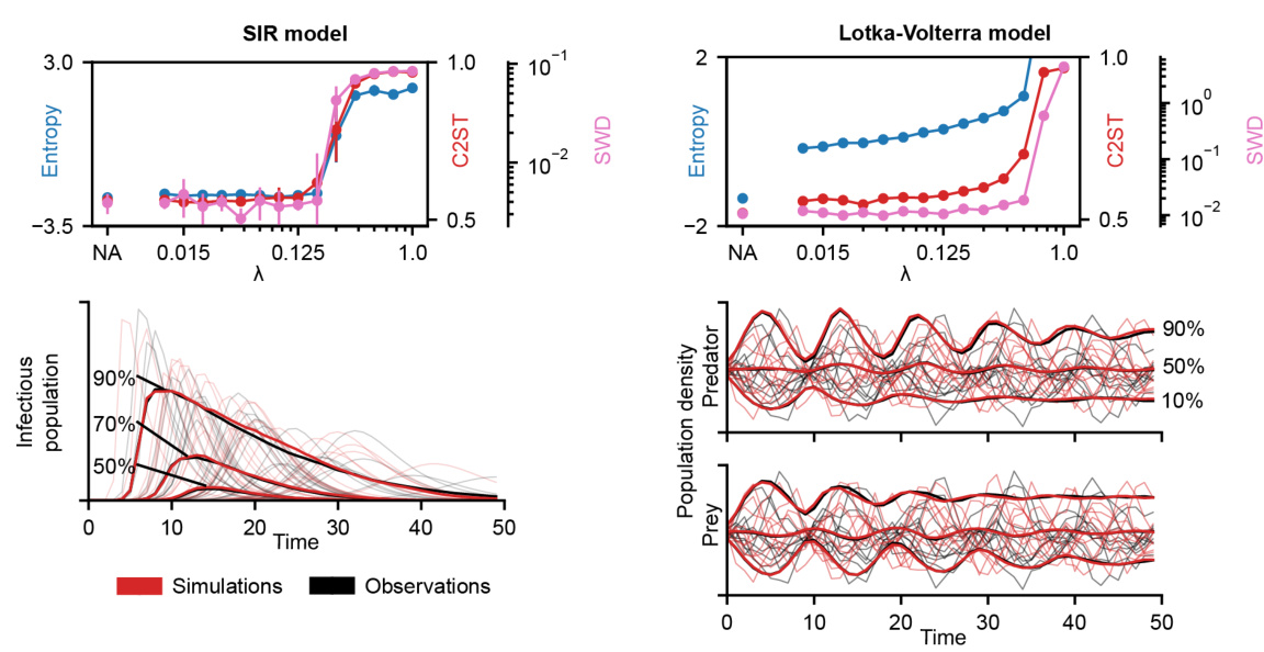
🔼 This figure displays the results of applying the Sourcerer method to two high-dimensional differentiable simulators: a deterministic SIR model and a probabilistic Lotka-Volterra model. The plots show the Sliced-Wasserstein distance (a measure of the discrepancy between the observed data distribution and the distribution of simulations generated by the estimated source) and the entropy of the estimated source distributions for different values of the regularization parameter λ. A higher entropy indicates more uncertainty in the estimated parameters, while a lower SWD indicates a better fit to the observed data. The figure demonstrates the impact of the entropy regularization on both the accuracy (SWD) and uncertainty (entropy) of source estimation, highlighting the ability of the method to increase the entropy of the estimated distributions without sacrificing accuracy.
read the caption
Figure 4: Source estimation on differentiable simulators. For both the deterministic SIR model (a) and probabilistic Lotka-Volterra model (b), the Sliced-Wasserstein distance (lower is better) between observations and simulations as well as entropy of estimated sources (higher is better) for different choices of λ and without the entropy regularization (NA) are shown. Mean and standard deviation are computed over five runs.

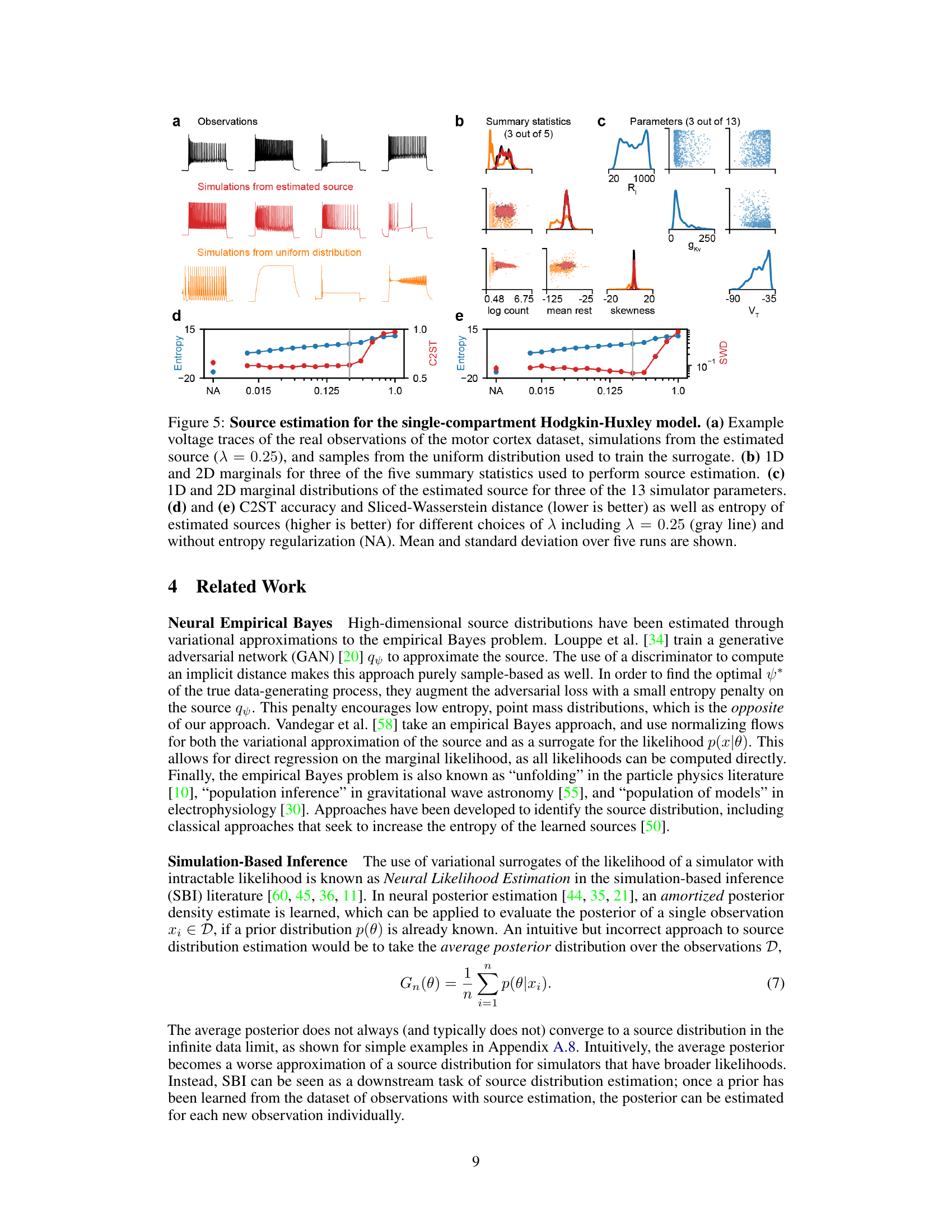
🔼 This figure shows the results of applying the Sourcerer method to a real-world dataset of electrophysiological recordings from the mouse motor cortex using a single-compartment Hodgkin-Huxley model. Panel (a) compares example voltage traces from real observations, simulations using the estimated source distribution, and simulations from a uniform prior distribution. Panels (b) and (c) show the marginal distributions of the summary statistics (used for model fitting) and the estimated parameters, respectively. Panels (d) and (e) display the C2ST accuracy, entropy, and SWD for varying regularization strength (λ), highlighting the benefit of entropy regularization in achieving high-entropy, accurate source estimates.
read the caption
Figure 5: Source estimation for the single-compartment Hodgkin-Huxley model. (a) Example voltage traces of the real observations of the motor cortex dataset, simulations from the estimated source (λ = 0.25), and samples from the uniform distribution used to train the surrogate. (b) 1D and 2D marginals for three of the five summary statistics used to perform source estimation. (c) 1D and 2D marginal distributions of the estimated source for three of the 13 simulator parameters. (d) and (e) C2ST accuracy and Sliced-Wasserstein distance (lower is better) as well as entropy of estimated sources (higher is better) for different choices of λ including λ = 0.25 (gray line) and without entropy regularization (NA). Mean and standard deviation over five runs are shown.

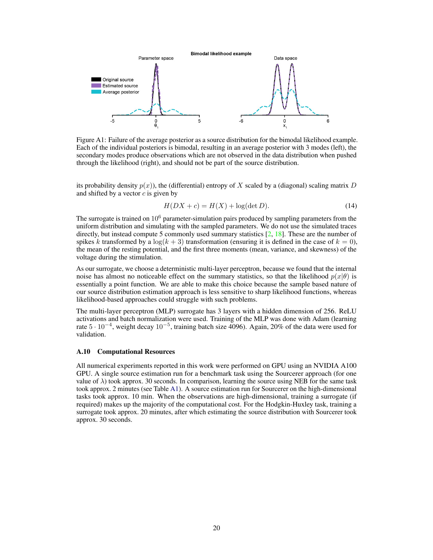
🔼 This figure demonstrates the failure of the average posterior to represent the source distribution for a bimodal likelihood. The average posterior is multimodal whereas the estimated source and original source are unimodal. This illustrates that simply averaging posteriors is not a reliable method for source estimation. The figure highlights that the average posterior includes modes that are not supported by the data distribution when passing through the likelihood function, showing that it is not a valid representation of the underlying source distribution.
read the caption
Figure A1: Failure of the average posterior as a source distribution for the bimodal likelihood example. Each of the individual posteriors is bimodal, resulting in an average posterior with 3 modes (left), the secondary modes produce observations which are not observed in the data distribution when pushed through the likelihood (right), and should not be part of the source distribution.
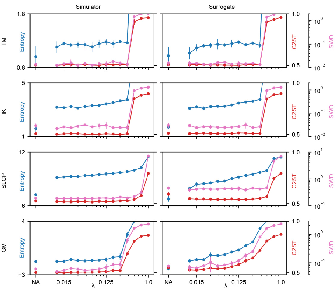
🔼 This figure presents the results of a source estimation benchmark comparing the proposed Sourcerer method against Neural Empirical Bayes (NEB). Panel (a) shows an example of the original and estimated source distributions for the inverse kinematics (IK) task, highlighting the increase in entropy achieved by Sourcerer without sacrificing accuracy. Panel (b) provides a quantitative comparison across four benchmark tasks (two moons, IK, SLCP, and Gaussian mixture), demonstrating Sourcerer’s superior performance in terms of both C2ST accuracy and entropy across various regularization strengths.
read the caption
Figure 3: Results for the source estimation benchmark. (a) Original and estimated source and corresponding pushforward for the differentiable IK simulator (λ = 0.35). The estimated source has higher entropy than the original source that was used to generate the data. The observations (simulated with parameters from the original source) and simulations (simulated with parameters from the estimated source) match. (b) Performance of our approach for all four benchmark tasks (TM, IK, SLCP, GM) using both the original (differentiable) simulators, and learned surrogates. Source estimation is performed without (NA) and with entropy regularization for different choices of λ. For all cases, mean C2ST accuracy between observations and simulations (lower is better) as well as the mean entropy of estimated sources (higher is better) over five runs are shown together with the standard deviation. The gray line at λ = 0.35 (λ = 0.062 for GM) indicates our choice of final λ for the numerical benchmark results (Table 1).
🔼 The figure displays the results of the source estimation benchmark comparing the proposed method Sourcerer to the Neural Empirical Bayes method. Panel (a) shows a specific example for the inverse kinematics task, illustrating that the estimated source distribution has higher entropy while maintaining data fidelity compared to the original source. Panel (b) provides a quantitative comparison across four different benchmark tasks, showing Sourcerer’s superior performance in terms of higher entropy in the estimated sources without compromising simulation accuracy as measured by the classifier two-sample test (C2ST). The impact of entropy regularization (λ) is also evaluated.
read the caption
Figure 3: Results for the source estimation benchmark. (a) Original and estimated source and corresponding pushforward for the differentiable IK simulator (λ = 0.35). The estimated source has higher entropy than the original source that was used to generate the data. The observations (simulated with parameters from the original source) and simulations (simulated with parameters from the estimated source) match. (b) Performance of our approach for all four benchmark tasks (TM, IK, SLCP, GM) using both the original (differentiable) simulators, and learned surrogates. Source estimation is performed without (NA) and with entropy regularization for different choices of λ. For all cases, mean C2ST accuracy between observations and simulations (lower is better) as well as the mean entropy of estimated sources (higher is better) over five runs are shown together with the standard deviation. The gray line at λ = 0.35 (λ = 0.062 for GM) indicates our choice of final λ for the numerical benchmark results (Table 1).

🔼 The figure displays results of the source estimation benchmark. The left panel (a) illustrates the original and estimated source distribution and the corresponding simulation results for one of the four benchmark tasks. The right panel (b) provides a comparison of the performance of the proposed method Sourcerer against another state-of-the-art method NEB on all four benchmark tasks, evaluating both the original simulators and learned surrogates for different choices of the regularization parameter λ.
read the caption
Figure 3: Results for the source estimation benchmark. (a) Original and estimated source and corresponding pushforward for the differentiable IK simulator (λ = 0.35). The estimated source has higher entropy than the original source that was used to generate the data. The observations (simulated with parameters from the original source) and simulations (simulated with parameters from the estimated source) match. (b) Performance of our approach for all four benchmark tasks (TM, IK, SLCP, GM) using both the original (differentiable) simulators, and learned surrogates. Source estimation is performed without (NA) and with entropy regularization for different choices of λ. For all cases, mean C2ST accuracy between observations and simulations (lower is better) as well as the mean entropy of estimated sources (higher is better) over five runs are shown together with the standard deviation. The gray line at λ = 0.35 (λ = 0.062 for GM) indicates our choice of final λ for the numerical benchmark results (Table 1).

🔼 This figure shows the results of the source estimation benchmark comparing the proposed Sourcerer method against Neural Empirical Bayes (NEB). The left panel (a) displays original and estimated source distributions for one task (inverse kinematics) showcasing that Sourcerer produces higher entropy estimates without sacrificing accuracy. The right panel (b) provides a summary across four benchmark tasks, showing the performance of Sourcerer with and without entropy regularization for different values of the regularization parameter λ. The results demonstrate that Sourcerer consistently achieves higher entropy estimates with comparable or better accuracy than NEB.
read the caption
Figure 3: Results for the source estimation benchmark. (a) Original and estimated source and corresponding pushforward for the differentiable IK simulator (λ = 0.35). The estimated source has higher entropy than the original source that was used to generate the data. The observations (simulated with parameters from the original source) and simulations (simulated with parameters from the estimated source) match. (b) Performance of our approach for all four benchmark tasks (TM, IK, SLCP, GM) using both the original (differentiable) simulators, and learned surrogates. Source estimation is performed without (NA) and with entropy regularization for different choices of λ. For all cases, mean C2ST accuracy between observations and simulations (lower is better) as well as the mean entropy of estimated sources (higher is better) over five runs are shown together with the standard deviation. The gray line at λ = 0.35 (λ = 0.062 for GM) indicates our choice of final λ for the numerical benchmark results (Table 1).
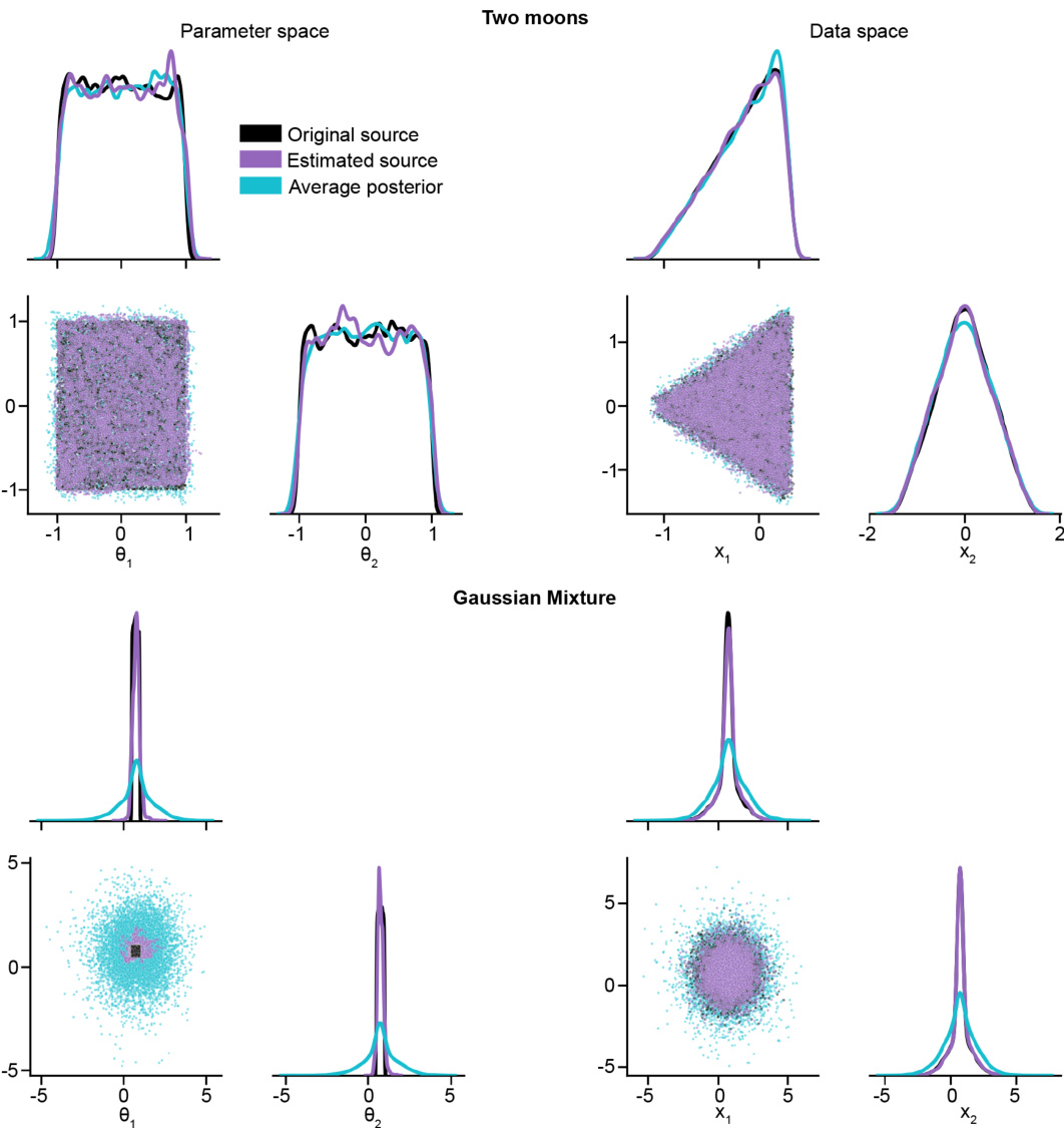
🔼 This figure presents the results of a source estimation benchmark comparing the proposed Sourcerer method to Neural Empirical Bayes (NEB). Panel (a) shows a specific example using the Inverse Kinematics (IK) simulator, illustrating that the estimated source distribution has higher entropy than the original, yet produces simulations matching the observations. Panel (b) provides a summary of results across four benchmark tasks (Two Moons, Inverse Kinematics, Simple Likelihood Complex Posterior, and Gaussian Mixture), comparing the methods with and without entropy regularization, and using both original and surrogate simulators. The results demonstrate that Sourcerer achieves comparable accuracy (C2ST) to NEB while consistently obtaining higher entropy source distributions.
read the caption
Figure 3: Results for the source estimation benchmark. (a) Original and estimated source and corresponding pushforward for the differentiable IK simulator (λ = 0.35). The estimated source has higher entropy than the original source that was used to generate the data. The observations (simulated with parameters from the original source) and simulations (simulated with parameters from the estimated source) match. (b) Performance of our approach for all four benchmark tasks (TM, IK, SLCP, GM) using both the original (differentiable) simulators, and learned surrogates. Source estimation is performed without (NA) and with entropy regularization for different choices of λ. For all cases, mean C2ST accuracy between observations and simulations (lower is better) as well as the mean entropy of estimated sources (higher is better) over five runs are shown together with the standard deviation. The gray line at λ = 0.35 (λ = 0.062 for GM) indicates our choice of final λ for the numerical benchmark results (Table 1).

🔼 This figure compares the original source distribution used to generate the data for the SLCP benchmark task with the estimated source distribution obtained using the Sourcerer method. The visualization shows that the estimated source distribution, while accurately reproducing the observed data distribution (in terms of the pushforward), has a higher entropy than the original source. This demonstrates Sourcerer’s ability to find a distribution that maintains higher uncertainty while still maintaining consistency with observations. The visualization displays marginal distributions of the 5 parameters for both the original and estimated sources.
read the caption
Figure A7: Original and estimated source distributions for the benchmark SLCP simulator. The estimated source has higher entropy than the original source.
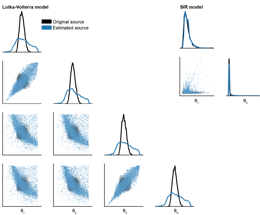
🔼 This figure visualizes the original and estimated source distributions for both the SIR and Lotka-Volterra models. For each model, it shows 1D marginal distributions and 2D scatter plots of the parameter pairs. The key observation is that for the Lotka-Volterra model, the estimated source distribution exhibits higher entropy (more spread out) than the original source distribution. This demonstrates the Sourcerer method’s ability to recover source distributions with higher entropy, while still maintaining fidelity to the observations.
read the caption
Figure A8: Original and estimated source distributions for the SIR and Lotka-Volterra model. For the Lotka-Volterra model, the estimated source has higher entropy than the original source.

🔼 This figure presents the results of a source estimation benchmark comparing the authors’ method (Sourcerer) to Neural Empirical Bayes (NEB). Panel (a) shows an example of the original and estimated source distributions and their corresponding pushforward distributions for a specific task (Inverse Kinematics), highlighting that Sourcerer yields a higher-entropy estimate without sacrificing accuracy. Panel (b) summarizes the results across four benchmark tasks, showing that Sourcerer consistently achieves higher entropy estimates and comparable accuracy to NEB, even when using surrogate models instead of the original differentiable simulators.
read the caption
Figure 3: Results for the source estimation benchmark. (a) Original and estimated source and corresponding pushforward for the differentiable IK simulator (λ = 0.35). The estimated source has higher entropy than the original source that was used to generate the data. The observations (simulated with parameters from the original source) and simulations (simulated with parameters from the estimated source) match. (b) Performance of our approach for all four benchmark tasks (TM, IK, SLCP, GM) using both the original (differentiable) simulators, and learned surrogates. Source estimation is performed without (NA) and with entropy regularization for different choices of λ. For all cases, mean C2ST accuracy between observations and simulations (lower is better) as well as the mean entropy of estimated sources (higher is better) over five runs are shown together with the standard deviation. The gray line at λ = 0.35 (λ = 0.062 for GM) indicates our choice of final λ for the numerical benchmark results (Table 1).
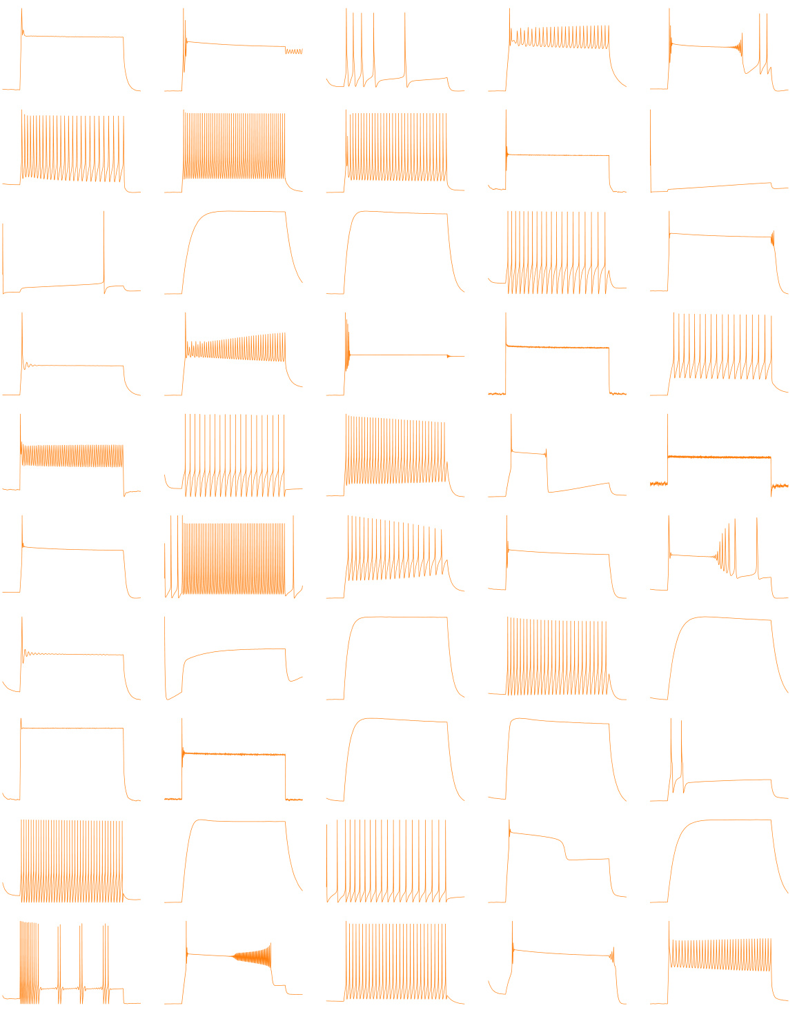
🔼 This figure shows the results of applying the Sourcerer method to estimate the source distribution for a single-compartment Hodgkin-Huxley model using real electrophysiological data. It compares voltage traces, summary statistics, and parameter distributions from the original recordings, the model estimated with and without entropy regularization, and a uniform distribution. It also evaluates the performance of this method using C2ST accuracy, Sliced-Wasserstein distance, and entropy.
read the caption
Figure 5: Source estimation for the single-compartment Hodgkin-Huxley model. (a) Example voltage traces of the real observations of the motor cortex dataset, simulations from the estimated source (λ = 0.25), and samples from the uniform distribution used to train the surrogate. (b) 1D and 2D marginals for three of the five summary statistics used to perform source estimation. (c) 1D and 2D marginal distributions of the estimated source for three of the 13 simulator parameters. (d) and (e) C2ST accuracy and Sliced-Wasserstein distance (lower is better) as well as entropy of estimated sources (higher is better) for different choices of λ including λ = 0.25 (gray line) and without entropy regularization (NA). Mean and standard deviation over five runs are shown.
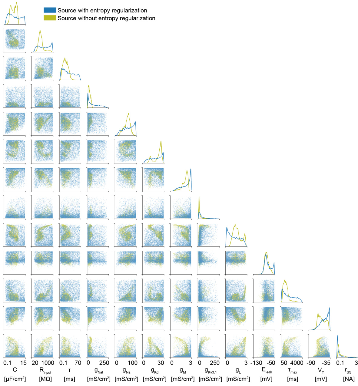
🔼 This figure shows the estimated source distributions for the parameters of the Hodgkin-Huxley model obtained with and without entropy regularization. The left panel displays the estimated source distributions when entropy regularization is applied (λ = 0.25). The right panel shows the estimated source distributions when no entropy regularization is applied. The visualization includes marginal distributions (histograms) for individual parameters along the diagonal and pairwise scatter plots for parameter pairs in the off-diagonal elements. Comparing both panels reveals that the entropy regularization helps to better explore the parameter space, leading to a more comprehensive estimate of the source distribution and potentially preventing biases from being introduced in downstream inference tasks.
read the caption
Figure A11: Estimated sources using for Hodgkin-Huxley task with the entropy regularization (λ = 0.25) and without the entropy regularization. Without, many viable parameter settings are missed, which would have significant downstream effects if the learned source distribution is used as a prior distribution for inference tasks.
More on tables

🔼 This table presents a quantitative comparison of the Sourcerer algorithm against the Neural Empirical Bayes (NEB) method across four benchmark tasks. The table displays the mean and standard deviation of the C2ST accuracy (a measure of how well the estimated source distribution reproduces the observed data) and the entropy (a measure of uncertainty) of the estimated source distributions for both differentiable simulators and surrogate models. The results highlight the ability of Sourcerer to achieve higher entropy without sacrificing accuracy, particularly when using entropy regularization.
read the caption
Table 1: Numerical benchmark results for Sourcerer. We show the mean and standard deviation over five runs for differentiable simulators and surrogates of Sourcerer on the benchmark tasks, and compare to NEB. All approaches achieve C2ST accuracies close to 50%. For the Sliced-Wasserstein-based approach, the entropies of the estimated sources are substantially higher (bold) with the entropy regularization (λ = 0.35 for TM, IK, SLCP, λ = 0.062 for GM, gray line in Fig. 3).

🔼 This table presents a quantitative comparison of Sourcerer’s performance against Neural Empirical Bayes (NEB) across four benchmark tasks. It shows the mean and standard deviation of C2ST accuracy (a measure of how well the simulations match the observations) and entropy (a measure of uncertainty) for both differentiable simulators and their learned surrogates, with and without entropy regularization. The results highlight Sourcerer’s ability to achieve high entropy without sacrificing simulation fidelity, especially when entropy regularization is used.
read the caption
Table 1: Numerical benchmark results for Sourcerer. We show the mean and standard deviation over five runs for differentiable simulators and surrogates of Sourcerer on the benchmark tasks, and compare to NEB. All approaches achieve C2ST accuracies close to 50%. For the Sliced-Wasserstein-based approach, the entropies of the estimated sources are substantially higher (bold) with the entropy regularization (λ = 0.35 for TM, IK, SLCP, λ = 0.062 for GM, gray line in Fig. 3).
Full paper#
