TL;DR#
Non-parametric classification methods struggle with high dimensionality and complex data structures. Existing techniques often suffer from slow convergence rates or fail to effectively capture the underlying data geometry, particularly when data lies on low-dimensional manifolds. This is a significant challenge because many real-world datasets exhibit such characteristics.
This paper presents two novel non-parametric classification algorithms based on the expand-and-sparsify (EaS) representation, which maps data points to a high-dimensional sparse representation. The first algorithm utilizes a winners-take-all sparsification step and achieves minimax-optimal convergence for data in general high-dimensional spaces. The second algorithm employs empirical k-thresholding and achieves minimax-optimal convergence rate, dependent only on the intrinsic dimension, for data residing on a low-dimensional manifold. Both algorithms are shown to be consistent and exhibit promising performance in empirical evaluations across multiple datasets.
Key Takeaways#
Why does it matter?#
This paper is crucial for researchers in non-parametric classification and high-dimensional data analysis. It introduces novel algorithms that leverage expand-and-sparsify representation, achieving minimax-optimal convergence rates. This work opens avenues for developing more efficient and accurate classifiers, particularly for data lying on low-dimensional manifolds. The theoretical findings are supported by empirical results, making it a valuable contribution to the field.
Visual Insights#
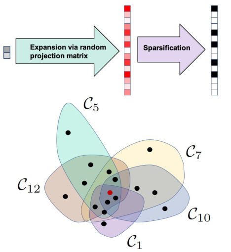
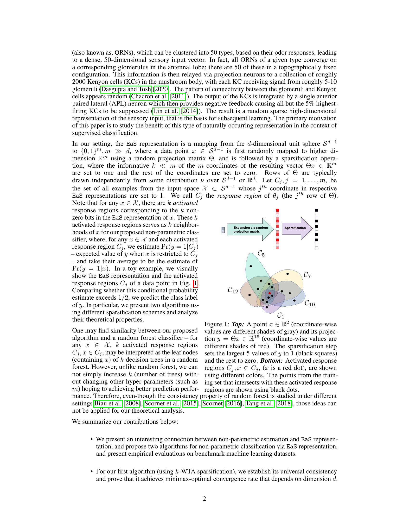
🔼 This figure illustrates the expand-and-sparsify (EaS) representation of a data point. The top part shows a 2D point being randomly projected into a higher 15D space. The sparsification process then selects the top 5 largest values and sets them to 1 (shown as black squares), setting the rest to zero. The bottom part depicts the activated response regions (Cj) in the original 2D space, which serve as neighborhoods for the data point (shown as a red dot). Black dots represent training data points that fall within these regions.
read the caption
Figure 1: Top: A point x ∈ R2 (coordinate-wise values are different shades of gray) and its projection y = Θx ∈ R15 (coordinate-wise values are different shades of red). The sparsification step sets the largest 5 values of y to 1 (black squares) and the rest to zero. Bottom: Activated response regions Cj, x ∈ Cj, (x is a red dot), are shown using different colors. The points from the training set that intersects with these activated response regions are shown using black dots.

🔼 The table lists eight datasets used in the paper’s empirical evaluation. For each dataset, the number of samples and the number of features are provided. The datasets include both real-world datasets (e.g., MNIST, Fashion-MNIST, Wine) and a synthetic dataset (twomoons). Some datasets have been pre-processed (e.g., dimensionality reduction for MNIST and Fashion-MNIST).
read the caption
Table 1: Dataset statistics
In-depth insights#
EaS Representation#
The expand-and-sparsify (EaS) representation offers a unique approach to data transformation for classification tasks. It begins by randomly projecting a low-dimensional data point into a significantly higher-dimensional space. This expansion step is followed by sparsification, where only the most informative features (coordinates) are retained, typically by setting a select few to ‘1’ and the rest to ‘0’. This process creates a sparse, high-dimensional representation that has shown promising benefits in capturing complex relationships in data. The random projection ensures robustness to noise and potential variations in data. The sparsification step is crucial in dimensionality reduction and enhancing computational efficiency. The EaS representation’s success hinges on carefully choosing the parameters (such as projection dimension and sparsity level) to optimize classifier performance and balance the tradeoff between representational power and computational demands. The method shows theoretical minimax optimality under certain assumptions, indicating its effectiveness in various scenarios.
Algorithm Analysis#
A thorough algorithm analysis would dissect the core components of the proposed algorithms, evaluating their computational complexity, memory usage, and scalability. For non-parametric classification algorithms, the focus would shift to evaluating the convergence rates, the impact of dimensionality on performance, and the robustness against noise and outliers. Specific attention should be given to the expand-and-sparsify representation, analyzing how the choice of expansion dimension and sparsification technique influence the classifier’s accuracy and efficiency. The analysis should compare the theoretical convergence rates with empirical results obtained from real-world datasets, potentially highlighting any discrepancies and suggesting avenues for improvement. Furthermore, a rigorous evaluation of the minimax optimality claim, verifying that the proposed methods achieve the optimal convergence rate in various scenarios, would be crucial. Finally, it would be insightful to analyze the algorithm’s ability to adapt to low-dimensional manifold structures and quantify this adaptability to showcase its effectiveness in handling high-dimensional data with intrinsic low dimensionality.
Manifold Learning#
Manifold learning is a powerful technique in machine learning that deals with high-dimensional data. It leverages the idea that high-dimensional data often lies on a low-dimensional manifold embedded within the higher-dimensional space. The core goal is to reduce the dimensionality of the data while preserving its essential structure and properties. This dimensionality reduction is achieved by learning the underlying manifold, which can significantly improve the performance of various machine learning algorithms by reducing computational complexity and mitigating the curse of dimensionality. Popular manifold learning techniques include Isomap, Locally Linear Embedding (LLE), Laplacian Eigenmaps, and t-distributed Stochastic Neighbor Embedding (t-SNE). Each method has unique strengths and weaknesses, and the optimal choice depends on the specific characteristics of the data and the desired outcome. Isomap aims to preserve geodesic distances between data points. LLE focuses on reconstructing each data point from its local neighbors. Laplacian Eigenmaps utilize graph Laplacian to capture the local geometry. t-SNE is particularly effective for visualization, but computationally expensive for large datasets. Despite their differences, these techniques are valuable for applications such as data visualization, clustering, classification, and feature extraction. Careful consideration of the computational cost and the interpretability of the results are critical when selecting a manifold learning method.
Empirical Results#
The empirical results section of a research paper is crucial for validating the theoretical claims. A strong empirical results section would present results from multiple datasets, demonstrating the generalizability of the proposed method and comparing its performance to existing state-of-the-art approaches. Robustness checks, such as varying hyperparameters or testing under noisy conditions, are essential for evaluating the method’s reliability. Clear visualization techniques like graphs and tables should present the findings effectively, allowing the reader to draw insightful comparisons and understand any limitations. Moreover, statistical significance testing is paramount to ensure that observed differences are not due to random chance, and the paper should clearly state the methods used. Ideally, the results should show a clear trend supporting the core hypothesis, but the section should also discuss any unexpected outcomes or limitations, reinforcing the paper’s honesty and promoting trust in the results. A thoughtful discussion of the results, contextualizing them in relation to prior work, and suggesting future avenues of research is essential for enhancing the impact of the findings.
Future Work#
The paper’s ‘Future Work’ section would benefit from exploring data-dependent projection direction choices for sparse representations. This would allow the model to adapt better to manifold structures, potentially mitigating the high constant in the excess Bayes risk bound that currently depends exponentially on the ambient dimension. Another avenue is investigating different sparsification schemes beyond k-winners-take-all and k-thresholding to further improve performance and explore the trade-offs between sparsity and accuracy. Finally, a focus on practical implementations and scalability is warranted. The theoretical results are strong but require further validation with large-scale datasets and analysis on how hyperparameters affect performance across various datasets and applications. Specifically, exploring the impact of m and k selection, and how they influence runtime and memory consumption, would be extremely beneficial.
More visual insights#
More on figures

🔼 This figure compares the performance of the proposed algorithm (Alg. 1) against k-Nearest Neighbors (k-NN) and Random Forest (RF) classifiers on eight different datasets. The x-axis represents the expansion factor (m/d), which is the ratio of the projection dimensionality (m) to the original dimensionality (d). The y-axis represents the test accuracy of each classifier. Error bars are included for Alg. 1 to show variability across 10 independent runs. The figure illustrates how the accuracy of Alg. 1 improves with increasing expansion factor, eventually becoming comparable to k-NN and RF.
read the caption
Figure 2: Empirical evaluation of Alg. 1, k-NN (for k = 1 and 10) and RF on eight datasets Here expansion factor is m/d. An error bar in the form of a shaded graph is provided for Alg. 1 over 10 independent runs.
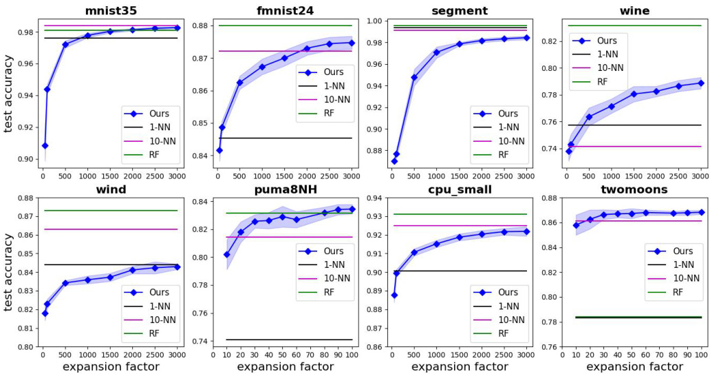
🔼 This figure compares the performance of the proposed algorithm (Alg. 1) with k-NN and random forest (RF) on eight benchmark datasets. The x-axis represents the expansion factor (m/d), which is a key hyperparameter in Alg. 1. The y-axis shows the test accuracy achieved by each method. Error bars are included for Alg. 1, representing results from 10 independent runs to demonstrate the variability. The results indicate how the proposed algorithm’s performance changes with varying levels of dimensionality expansion and compares its accuracy to other commonly used non-parametric methods.
read the caption
Figure 2: Empirical evaluation of Alg. 1, k-NN (for k = 1 and 10) and RF on eight datasets Here expansion factor is m/d. An error bar in the form of a shaded graph is provided for Alg. 1 over 10 independent runs.
Full paper#

