TL;DR#
Current methods for protein representation learning struggle to effectively capture the intricate interplay between a protein’s sequence and its 3D structure, limiting their performance in tasks like protein function prediction. This paper addresses this issue by highlighting the absence of practical methods for modeling the interdependencies between protein sequences and structures.
The proposed solution, CoupleNet, tackles this challenge by dynamically integrating sequence and structural features at multiple levels. This is achieved through a novel two-type dynamic graph that captures both local and global relationships, coupled with concurrent convolutions on nodes and edges. Experimental results demonstrate CoupleNet’s superior performance compared to existing methods, especially when dealing with proteins exhibiting low sequence similarities. This approach provides a more comprehensive and accurate representation of proteins, leading to improved accuracy in protein function prediction.
Key Takeaways#
Why does it matter?#
This paper is crucial for researchers in protein science and machine learning. CoupleNet offers a novel approach to protein representation learning, significantly improving performance on various tasks, especially those involving low sequence similarity. This opens new avenues for research in protein function prediction, drug discovery, and understanding protein evolution. The dynamic graph construction and simultaneous node-edge convolution methods presented are also highly valuable for graph neural network researchers.
Visual Insights#
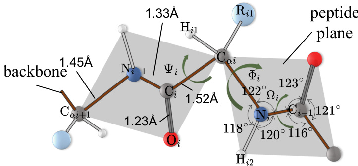
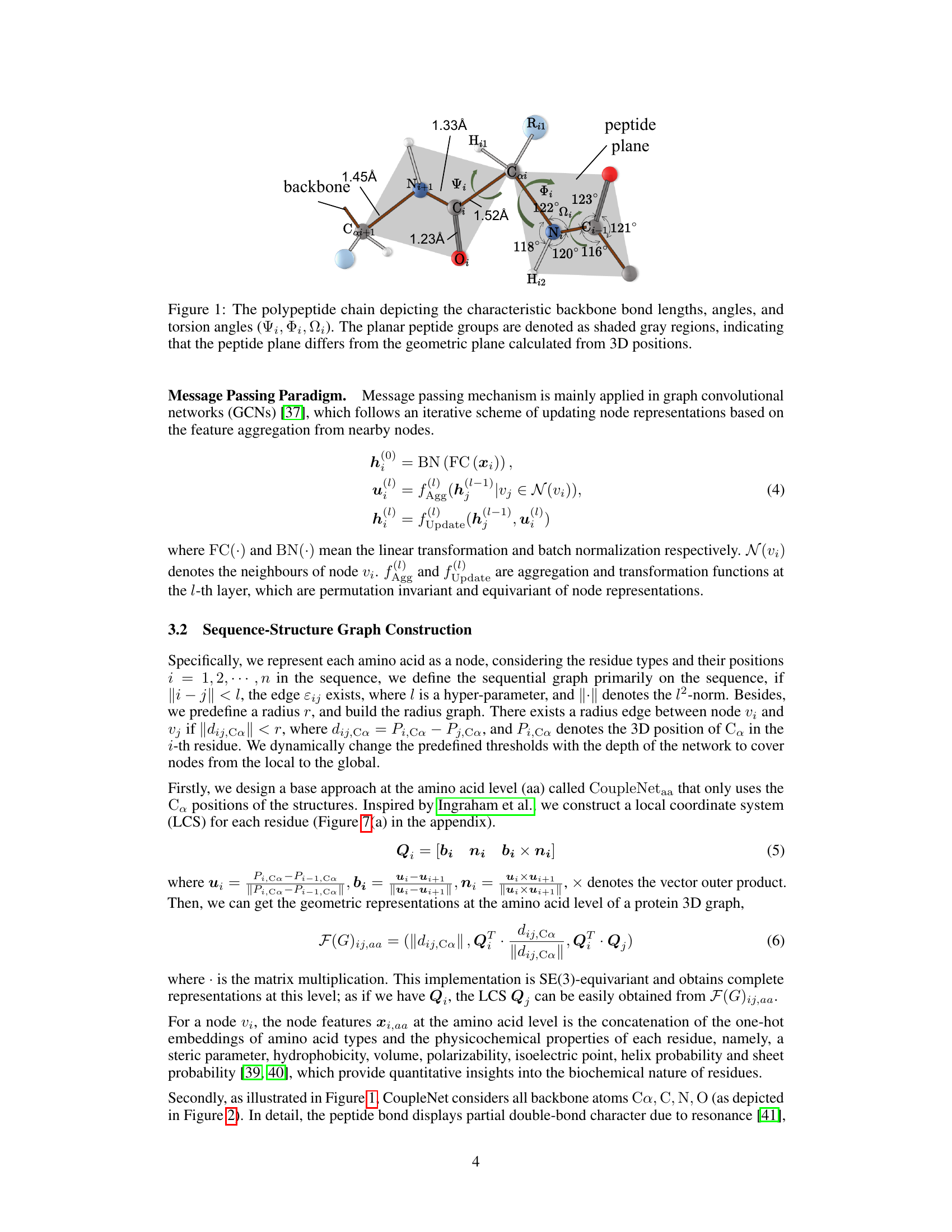
🔼 This figure illustrates the geometry of a polypeptide chain, highlighting key bond lengths, angles, and torsion angles (phi, psi, omega). The shaded gray regions emphasize the planarity of the peptide groups, contrasting with the overall three-dimensional structure. This geometry is fundamental to understanding protein structure and is used in CoupleNet’s construction of geometric features.
read the caption
Figure 1: The polypeptide chain depicting the characteristic backbone bond lengths, angles, and torsion angles (Ψi, Φi, Ωi). The planar peptide groups are denoted as shaded gray regions, indicating that the peptide plane differs from the geometric plane calculated from 3D positions.
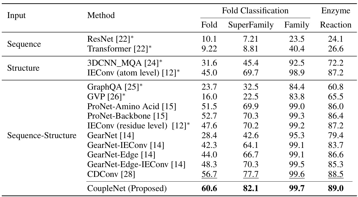
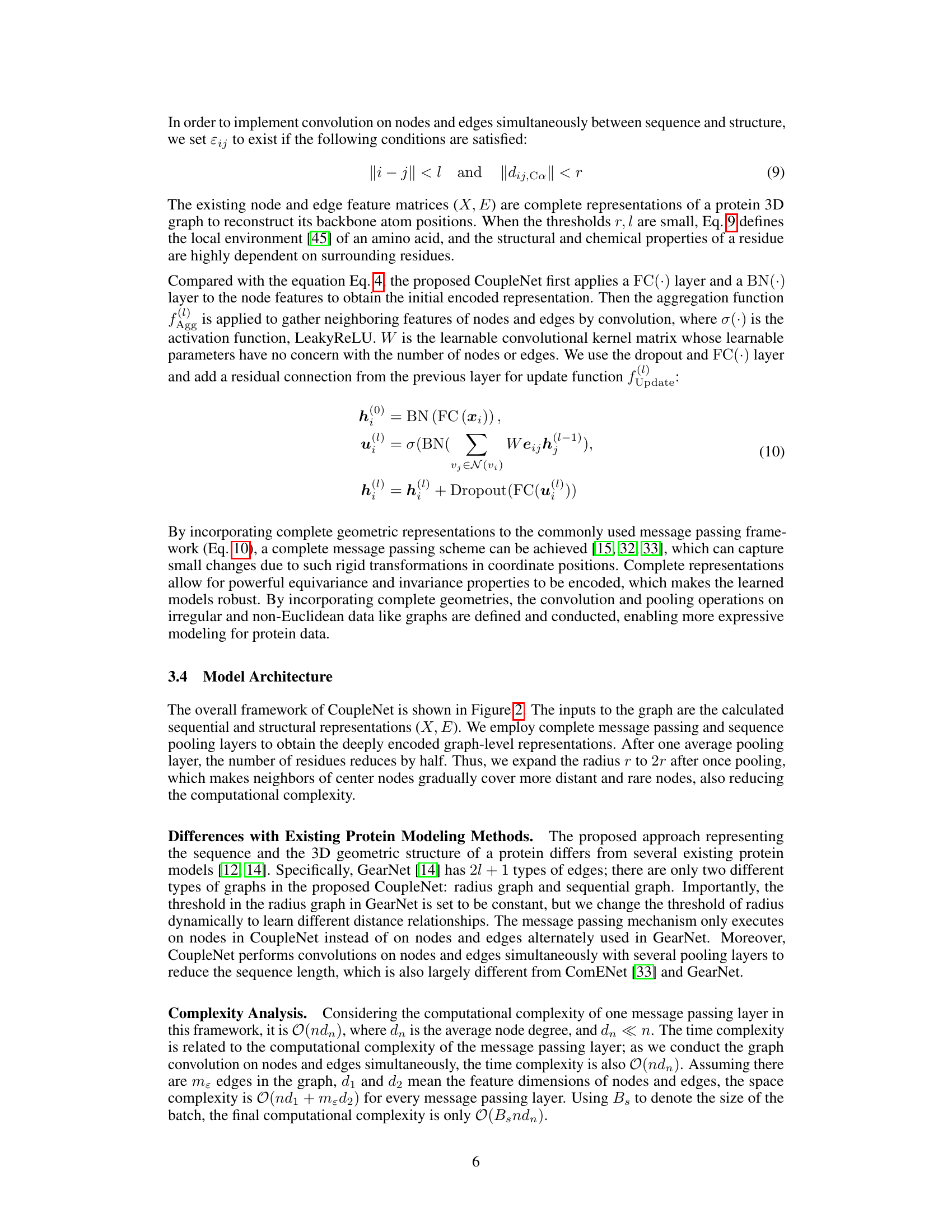
🔼 This table presents the accuracy of various methods on protein fold and enzyme reaction classification tasks. The accuracy is measured as a percentage. The table compares the performance of different methods, categorized by their input type (sequence only, structure only, or both sequence and structure), and highlights the best-performing method (CoupleNet) for each subtask (fold, superfamily, family, and reaction). The asterisk [*] indicates results obtained from a different source ([28]).
read the caption
Table 1: Accuracy (%) on fold classification and enzyme reaction classification. [*] denotes the results are taken from [28]. The best and suboptimal results are shown in bold and underline.
In-depth insights#
Sequence-Structure Coupling#
Sequence-structure coupling in protein representation learning aims to synergistically leverage the information encoded in both the amino acid sequence (1D) and the 3D structure of a protein. Direct concatenation of separate sequence and structure embeddings is insufficient, as it fails to capture the intricate dependencies between these two aspects. Effective coupling methods must explicitly model these relationships, often using graph neural networks (GNNs) or other techniques to integrate features from both domains. CoupleNet, for example, uses a dynamic graph approach to capture local and global interactions, enabling more comprehensive protein representation learning. Successful coupling methods often result in improved performance on downstream tasks, such as protein function prediction, particularly in scenarios involving low-sequence similarity where structural information becomes critical. The challenge remains in developing computationally efficient and robust methods to fully exploit the complexities of sequence-structure interplay for comprehensive protein understanding.
Dynamic Graph Networks#
Dynamic Graph Networks represent a powerful paradigm shift in graph-based machine learning, offering significant advantages over traditional static graph methods. Their dynamic nature allows them to adapt and evolve as new information becomes available, reflecting the inherent temporal and contextual changes within real-world networks. This adaptability is particularly crucial for modeling complex systems where relationships and structures shift over time. The ability to update node and edge features, add or remove nodes and edges, and adjust network topology enables a more accurate representation of the system’s dynamics. This adaptability is particularly important in applications such as social network analysis, where relationships constantly evolve, or in recommendation systems, where user preferences and item popularity change over time. Moreover, the introduction of dynamic graph structures facilitates the capture of long-range dependencies and subtle interactions that are often missed in static graphs. This improved accuracy has significant implications for downstream tasks such as prediction and forecasting. The key challenge remains in designing efficient algorithms for updating and managing the dynamic network, while maintaining computational tractability. Research in this area is focused on developing novel techniques that balance expressive power with scalability and efficiency.
Complete Geometric Features#
The concept of “Complete Geometric Features” in a protein structure analysis context suggests a method that captures the full spatial arrangement of atoms, going beyond limited local neighborhoods. This approach aims to provide a comprehensive, holistic representation of the protein’s 3D structure, enabling more accurate prediction of protein function and properties. Complete features might include not only atom positions and distances, but also various geometric descriptors such as bond angles, dihedral angles, and other relational information that reflects protein conformation. The completeness requirement likely addresses limitations of methods that only focus on local interactions, potentially missing long-range correlations essential for protein folding and dynamics. A successful method must be invariant to rigid-body transformations, ensuring that different orientations or translations of the same molecule generate identical feature representations. The challenge lies in efficiently computing and representing these features, especially for large proteins with many atoms. The value lies in their potential to significantly improve the accuracy and reliability of various protein analysis tasks, particularly in low-sequence-similarity scenarios where traditional sequence-based methods fall short. This holistic representation, therefore, is crucial for a more complete understanding of protein structure-function relationships.
CoupleNet Performance#
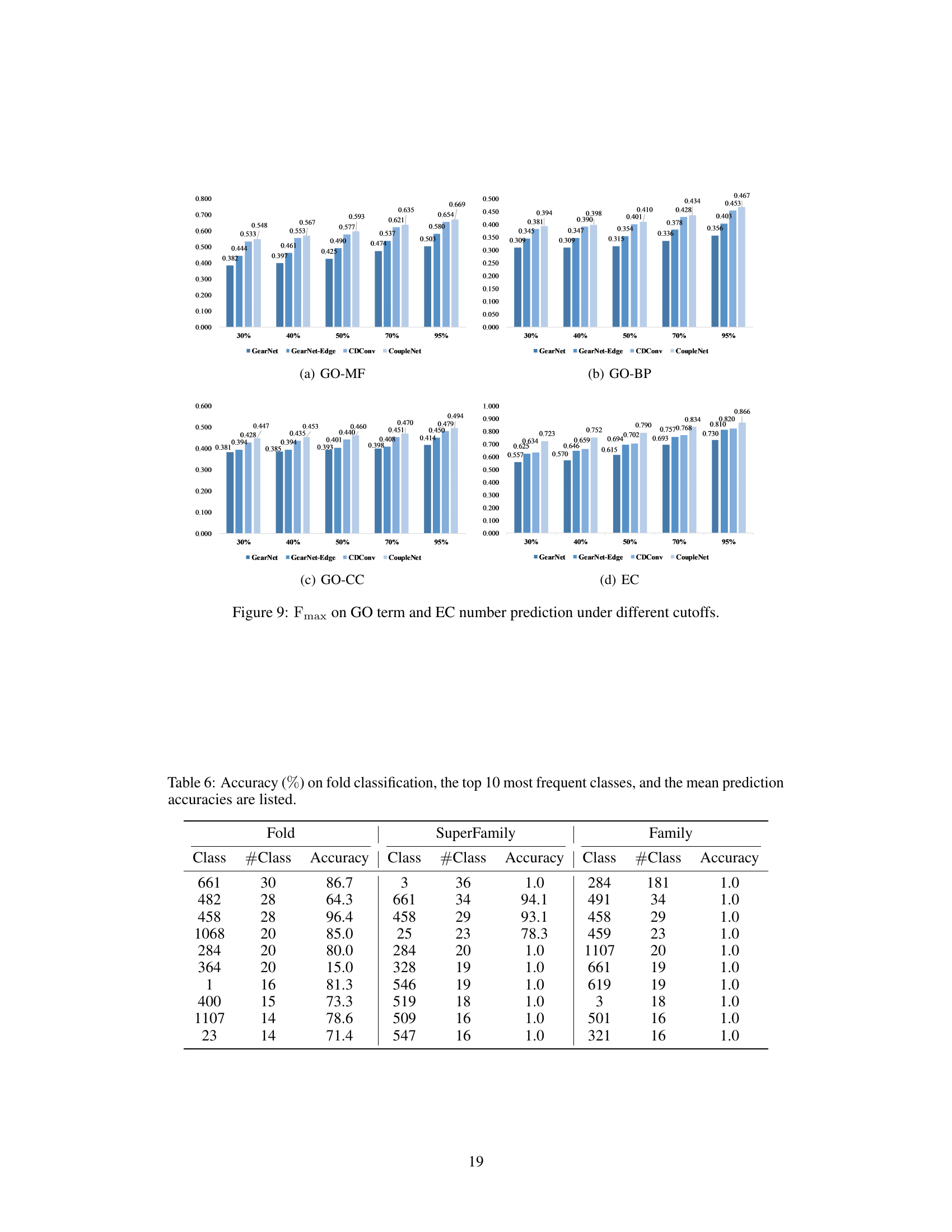
CoupleNet’s performance is a standout aspect of the research, showcasing significant improvements over existing state-of-the-art methods in protein representation learning. The model’s success is particularly notable in scenarios with low sequence similarity, where it adeptly identifies rarely encountered functions and captures remote homology relationships. This superior performance is attributed to CoupleNet’s novel architecture, which dynamically integrates protein sequence and structure information at multiple levels and scales. Simultaneous convolutions on nodes and edges within a dual-graph system ensure comprehensive feature extraction. The ability to handle various protein lengths effectively, exhibiting strong performance even with long sequences, is another significant advantage. The model’s robustness and accuracy across various benchmark datasets strongly suggest that its dynamic approach to integrating sequence and structural data results in highly informative protein representations with broad applicability.
Future Research#
Future research directions stemming from this CoupleNet work could explore several promising avenues. Improving efficiency is crucial; exploring more efficient graph convolutional techniques or alternative architectures that reduce computational complexity while maintaining accuracy is key. Expanding functionality beyond the current protein tasks (fold prediction, etc.) to encompass broader biological applications, like protein-protein interaction prediction or drug-target interaction modeling, is essential for wider impact. Enhancing data augmentation strategies, particularly those addressing the limitations of sparse and noisy protein data, would significantly boost performance. Addressing class imbalance problems inherent in protein datasets through advanced sampling techniques or loss functions could lead to more robust and generalizable results. Finally, integrating multi-modal information, incorporating other relevant data such as experimental data or evolutionary information, holds considerable potential for further accuracy gains and a deeper biological understanding. This multi-faceted approach would fully exploit the richness of available data, unlocking new insights into protein function and structure.
More visual insights#
More on figures

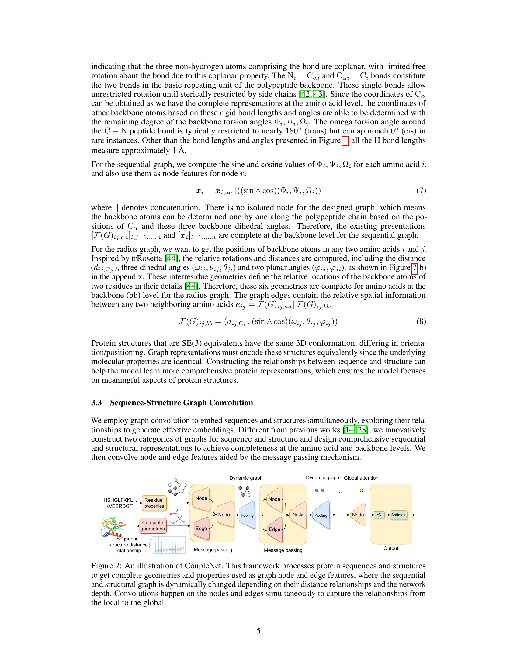
🔼 CoupleNet processes protein sequences and 3D structures. It uses a two-type dynamic graph to capture local and global relationships between sequence and structure features. Node and edge convolutions are performed simultaneously to generate comprehensive protein embeddings. The dynamic graph changes based on network depth and distance relationships, improving the modeling of node-edge relationships. The framework produces complete representations at amino acid and backbone levels.
read the caption
Figure 2: An illustration of CoupleNet. This framework processes protein sequences and structures to get complete geometries and properties used as graph node and edge features, where the sequential and structural graph is dynamically changed depending on their distance relationships and the network depth. Convolutions happen on the nodes and edges simultaneously to capture the relationships from the local to the global.
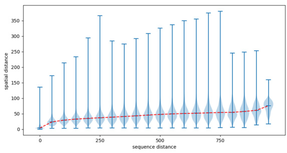
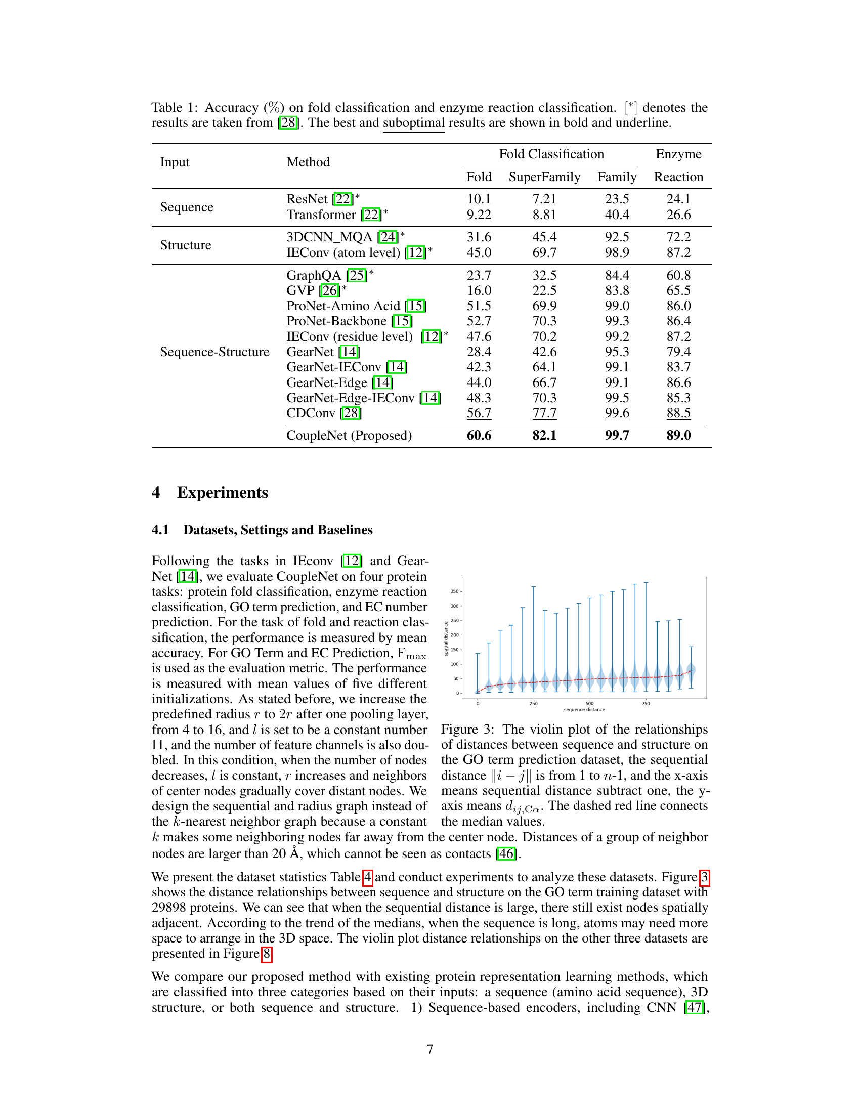
🔼 This figure shows the relationship between the sequential distance and the spatial distance between amino acids in proteins using a violin plot. The x-axis represents the sequential distance (i-j) between amino acid residues, indicating how far apart they are in the protein’s sequence. The y-axis shows the spatial distance (dij,Ca) between the Ca atoms of these residues in the protein’s 3D structure, indicating how far apart they are in space. The violin plot displays the distribution of spatial distances for each sequential distance, providing information about the range and frequency of spatial distances. The dashed red line connects the median spatial distance for each sequential distance. This visualization helps to understand how the spatial arrangement of amino acids in a protein’s 3D structure relates to their linear order in the protein sequence.
read the caption
Figure 3: The violin plot of the relationships of distances between sequence and structure on the GO term prediction dataset, the sequential distance ||i – j|| is from 1 to n-1, and the x-axis means sequential distance subtract one, the y-axis means dij, Ca. The dashed red line connects the median values.
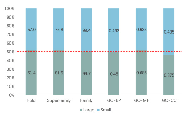
🔼 This figure shows the performance of CoupleNet on large and small proteins in terms of accuracy on various tasks. The x-axis shows the different tasks and the y-axis shows the percentage of proteins with sequence lengths above or below the mean for each task. The red line represents the 50% mark. It visualizes how the performance of CoupleNet varies with protein length, showing higher accuracy for larger proteins in some tasks but not a significant correlation in others.
read the caption
Figure 4: Percentage accumulation chart of results on large and small proteins. The vertical axis shows the percentage, where the red line indicates 50%.

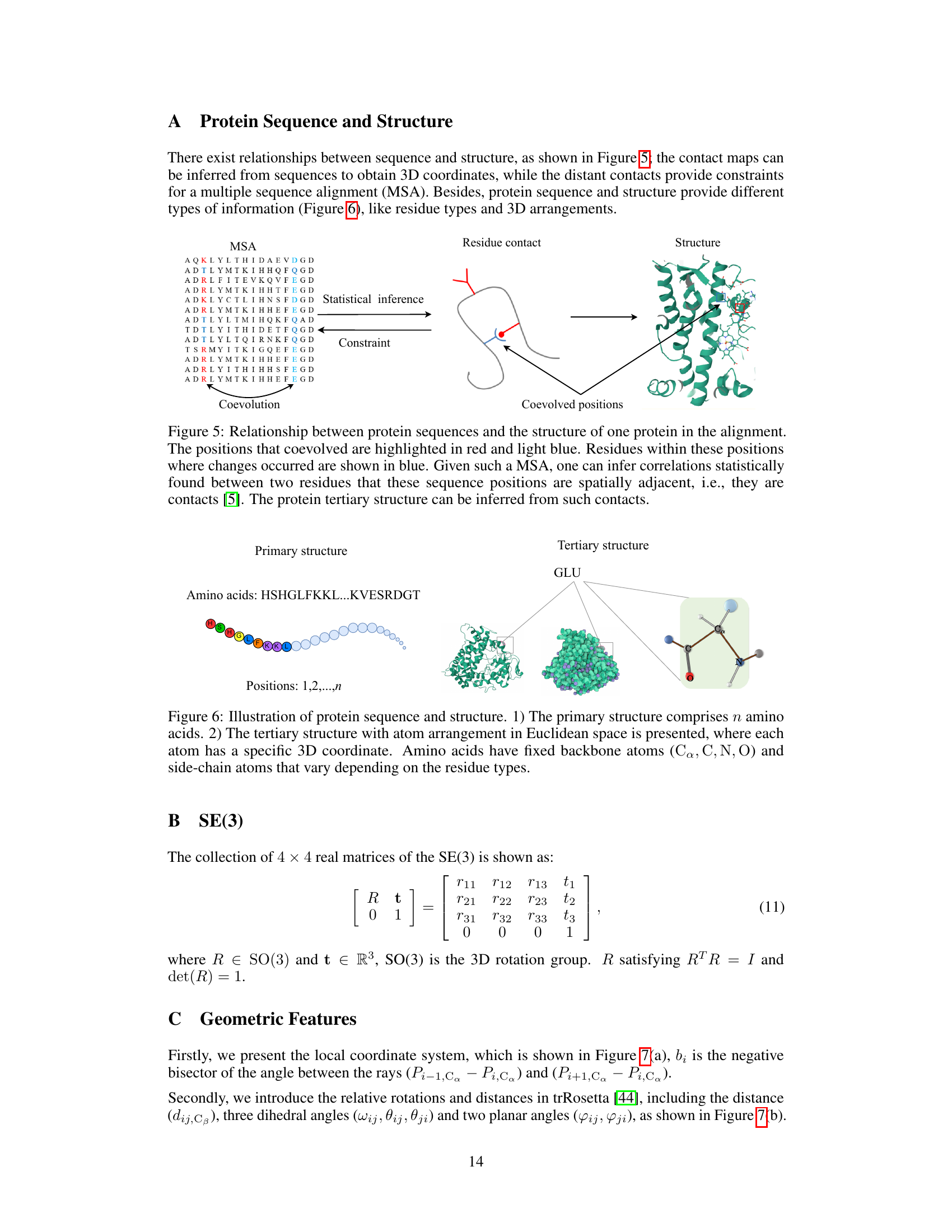
🔼 This figure demonstrates the relationship between protein sequences and their 3D structure. It highlights how co-evolved positions in a multiple sequence alignment (MSA) can be used to infer residue contacts, which in turn are used to predict the protein’s 3D structure. The colored residues in the MSA indicate the positions that coevolved, providing constraints for structure prediction.
read the caption
Figure 5: Relationship between protein sequences and the structure of one protein in the alignment. The positions that coevolved are highlighted in red and light blue. Residues within these positions where changes occurred are shown in blue. Given such a MSA, one can infer correlations statistically found between two residues that these sequence positions are spatially adjacent, i.e., they are contacts [5]. The protein tertiary structure can be inferred from such contacts.

🔼 This figure illustrates the difference between the primary and tertiary structures of a protein. The primary structure shows the linear sequence of amino acids, represented by colored circles. The tertiary structure depicts the 3D folded conformation of the protein, showing the spatial arrangement of atoms. The zoomed-in section shows the detail of the backbone atoms (Cα, C, N, O) and the side chains, which are variable and depend on the type of amino acid.
read the caption
Figure 6: Illustration of protein sequence and structure. 1) The primary structure comprises n amino acids. 2) The tertiary structure with atom arrangement in Euclidean space is presented, where each atom has a specific 3D coordinate. Amino acids have fixed backbone atoms (Ca, C, N, O) and side-chain atoms that vary depending on the residue types.
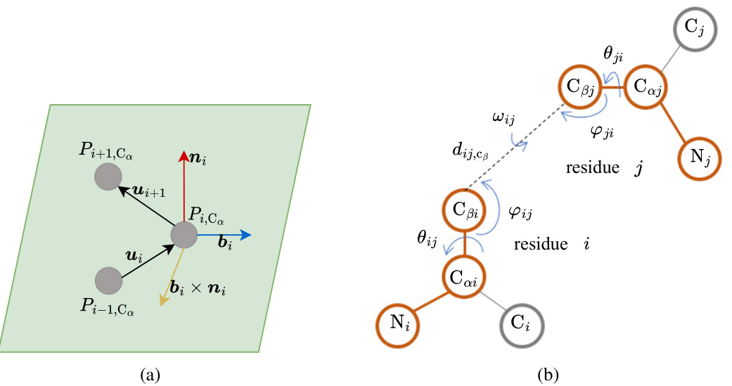
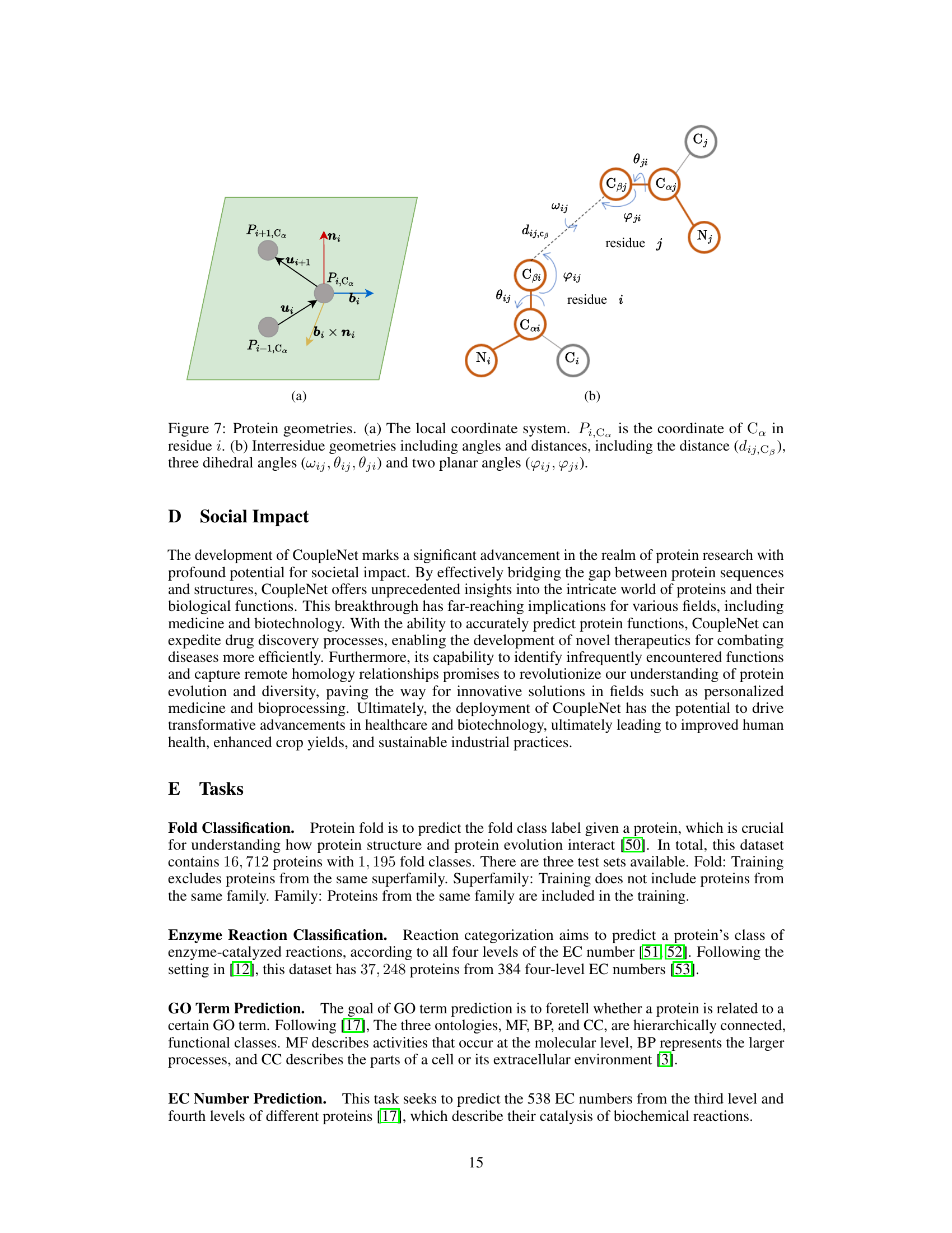
🔼 This figure shows the geometric features used in CoupleNet. Panel (a) illustrates the local coordinate system (LCS) created for each residue using the Cα atom positions of three consecutive residues. The LCS is defined by vectors bi and ni calculated from the relative positions. Panel (b) shows the inter-residue geometries including distances (dij,Cβ) and angles (ωij, θij, ψij, φij, γji) between the backbone atoms of two residues (i and j). These geometric features capture both local and global structural information.
read the caption
Figure 7: Protein geometries. (a) The local coordinate system. Pi,Ca is the coordinate of Cα in residue i. (b) Interresidue geometries including angles and distances, including the distance (dij,Cβ), three dihedral angles (ωij, θij, ψij) and two planar angles (φij, γji).
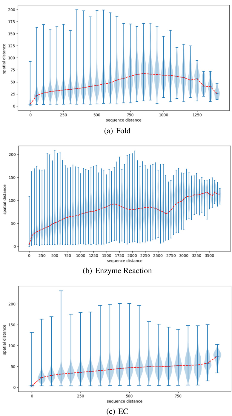
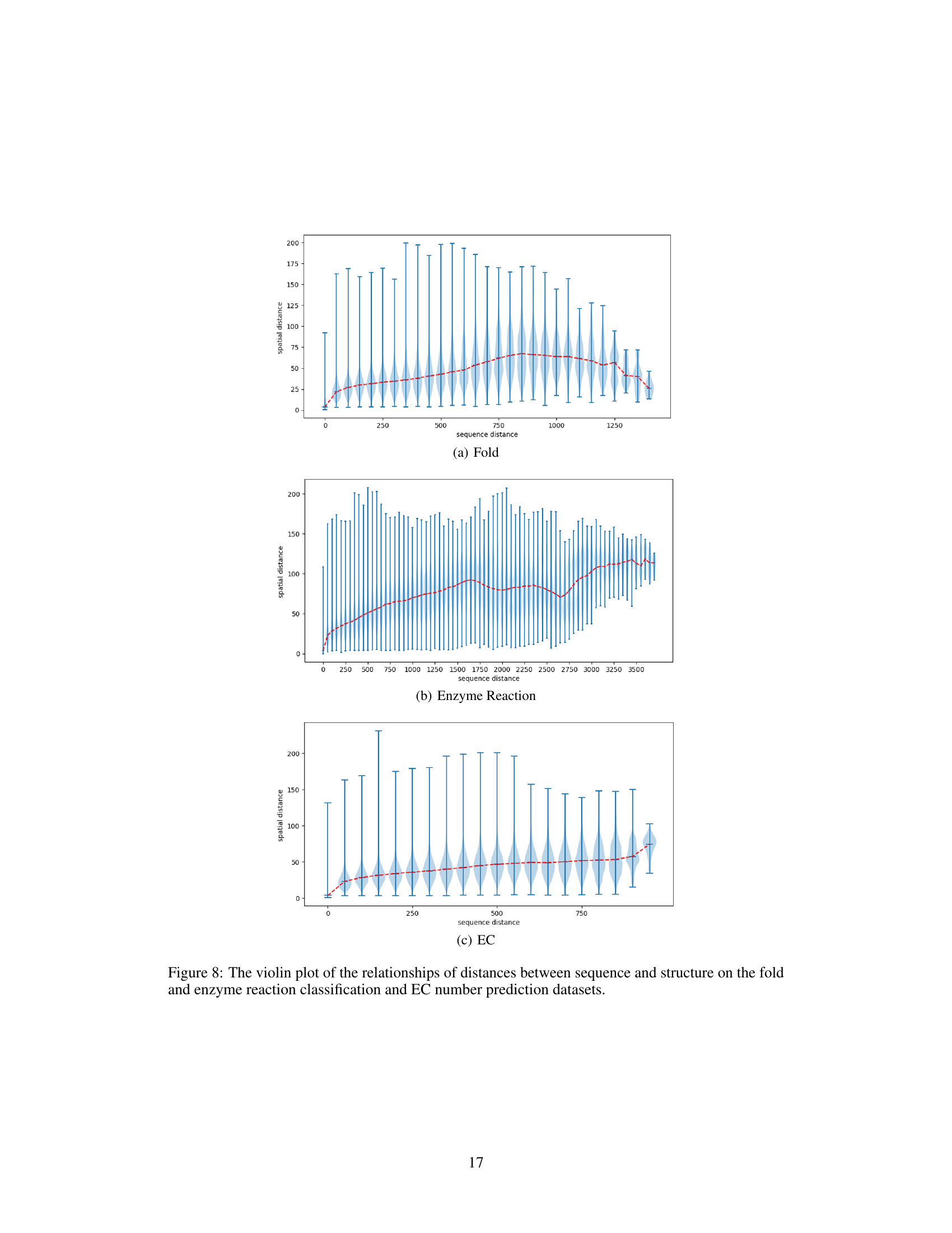
🔼 This figure presents violin plots illustrating the relationship between sequence distance and spatial distance for three different datasets: protein fold classification, enzyme reaction classification, and EC number prediction. Each violin plot shows the distribution of spatial distances (y-axis) for various sequence distances (x-axis). The red line represents the median spatial distance for each sequence distance, giving a visual representation of the trend. The plots aim to demonstrate how the spatial proximity of amino acids in 3D space relates to their sequential distance in the protein sequence, offering insights into the complex interplay between protein sequence and structure.
read the caption
Figure 8: The violin plot of the relationships of distances between sequence and structure on the fold and enzyme reaction classification and EC number prediction datasets.
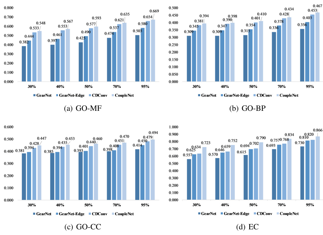
🔼 This figure shows violin plots illustrating the relationship between sequence distance and spatial distance for three different protein datasets: Fold, Enzyme Reaction, and EC Number prediction. Each plot displays the distribution of spatial distances (y-axis) for various sequence distances (x-axis). The plots reveal how the relationship between sequence and spatial distances varies across datasets, likely reflecting different structural organization patterns and constraints.
read the caption
Figure 8: The violin plot of the relationships of distances between sequence and structure on the fold and enzyme reaction classification and EC number prediction datasets.
More on tables
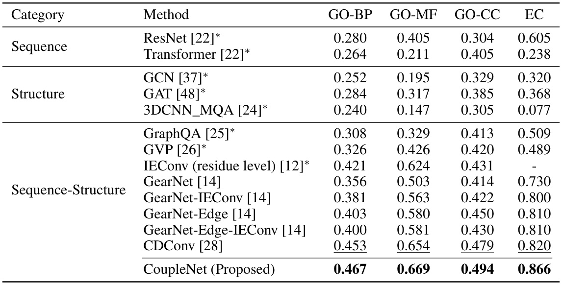
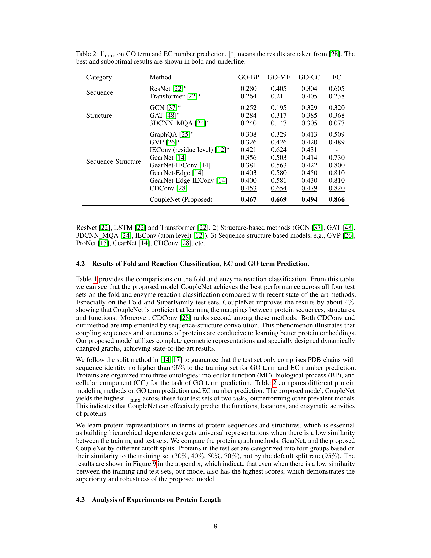
🔼 This table presents the Fmax scores achieved by various methods on Gene Ontology (GO) term prediction and Enzyme Commission (EC) number prediction tasks. The results are categorized by the type of input used (sequence only, structure only, or both sequence and structure). The best and second-best performing methods are highlighted in bold and underlined, respectively. The asterisk (*) indicates results that were obtained from a previous study (reference [28]).
read the caption
Table 2: Fmax on GO term and EC number prediction. [*] means the results are taken from [28]. The best and suboptimal results are shown in bold and underline.

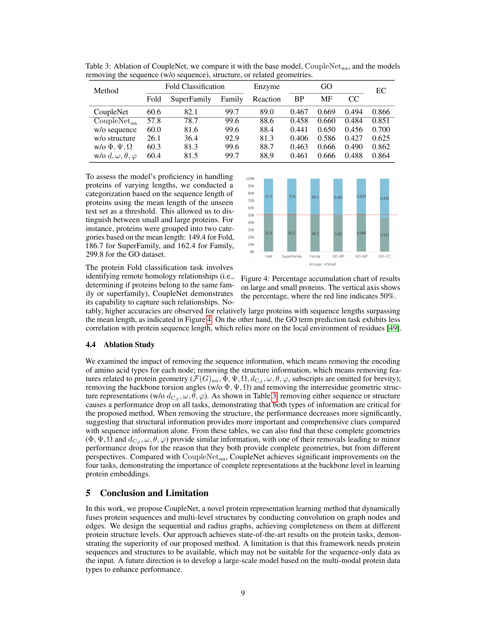
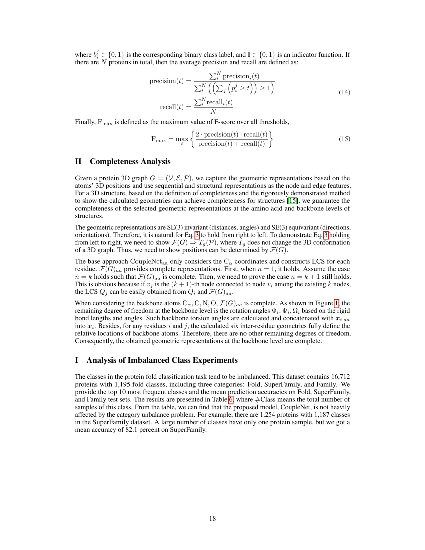
🔼 This table presents the results of ablation experiments on the CoupleNet model. It shows the performance of the full CoupleNet model and several variants where either the sequence information, the 3D structure information, or specific geometric features (backbone torsion angles or inter-residue geometries) are removed. The results are evaluated across various protein tasks, including fold classification, enzyme reaction classification, and gene ontology (GO) term prediction, allowing assessment of the contribution of different data modalities and features to overall model performance.
read the caption
Table 3: Ablation of CoupleNet, we compare it with the base model, CoupleNetaa, and the models removing the sequence (w/o sequence), structure, or related geometries.
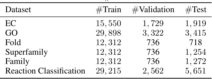
🔼 This table presents the accuracy results of different methods on protein fold classification and enzyme reaction classification tasks. The methods are categorized by the type of input data they use (sequence, structure, or both). The table shows the accuracy for each task and for different levels of granularity (Fold, SuperFamily, Family, Reaction). The best and second-best performing methods are highlighted.
read the caption
Table 1: Accuracy (%) on fold classification and enzyme reaction classification. [*] denotes the results are taken from [28]. The best and suboptimal results are shown in bold and underline.

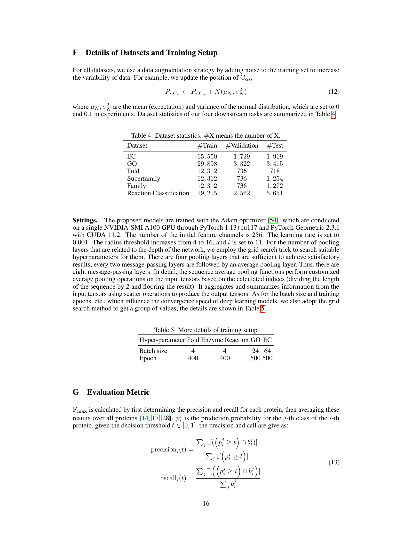
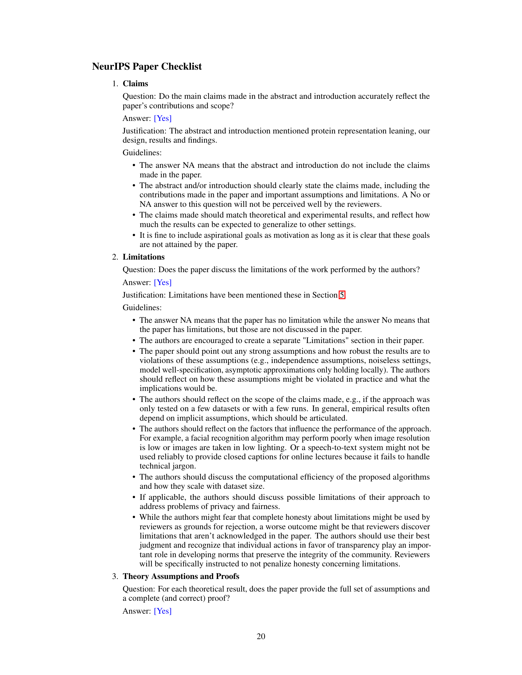
🔼 This table provides the hyperparameter settings used for training the CoupleNet model on different tasks. The hyperparameters listed are batch size and epoch, both of which are crucial for model training. Different settings were employed for the Fold, Enzyme Reaction, GO, and EC tasks, indicating task-specific optimization strategies.
read the caption
Table 5: More details of training setup
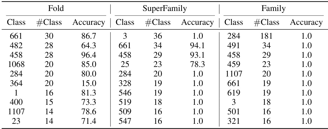
🔼 This table presents the accuracy of different methods on protein fold classification and enzyme reaction classification tasks. It compares the performance of various methods, including ResNet, Transformer, 3DCNN_MQA, IEConv, GraphQA, GVP, ProNet, GearNet, and CDConv, against the proposed CoupleNet model. The results are categorized by input type (sequence, structure, or both) and broken down further by specific classification tasks (fold, superfamily, family, and reaction). The best performing model in each category is highlighted in bold, and the second-best is underlined.
read the caption
Table 1: Accuracy (%) on fold classification and enzyme reaction classification. [*] denotes the results are taken from [28]. The best and suboptimal results are shown in bold and underline.
Full paper#

