TL;DR#
Many real-world machine learning applications face the challenge of adapting to continuously changing data distributions (non-stationary environments). Existing continual test-time adaptation methods often struggle with representation alignment, especially when unlabeled data are scarce. This makes it difficult to maintain optimal model performance over time, leading to issues such as catastrophic forgetting.
This research introduces Ada-ReAlign, a novel method to address these challenges. Ada-ReAlign uses a group of base learners to explore different parts of the unlabeled data stream, which are combined by a meta-learner to find an optimal balance between using historical data and recent observations. This adaptive approach effectively aligns unlabeled data with source data representations. The results demonstrate Ada-ReAlign’s superior performance compared to existing methods on benchmark datasets and in a real-world application, showcasing its robustness and adaptability in non-stationary environments.
Key Takeaways#
Why does it matter?#
This paper is crucial for researchers in machine learning and related fields because it tackles the critical challenge of continual adaptation in non-stationary environments, a common issue in real-world applications where data distributions constantly shift. The proposed Ada-ReAlign algorithm offers a novel approach with theoretical guarantees, addressing limitations of existing methods. Its effectiveness is validated on benchmark datasets and a real-world application, opening up avenues for more robust and adaptive machine learning systems.
Visual Insights#

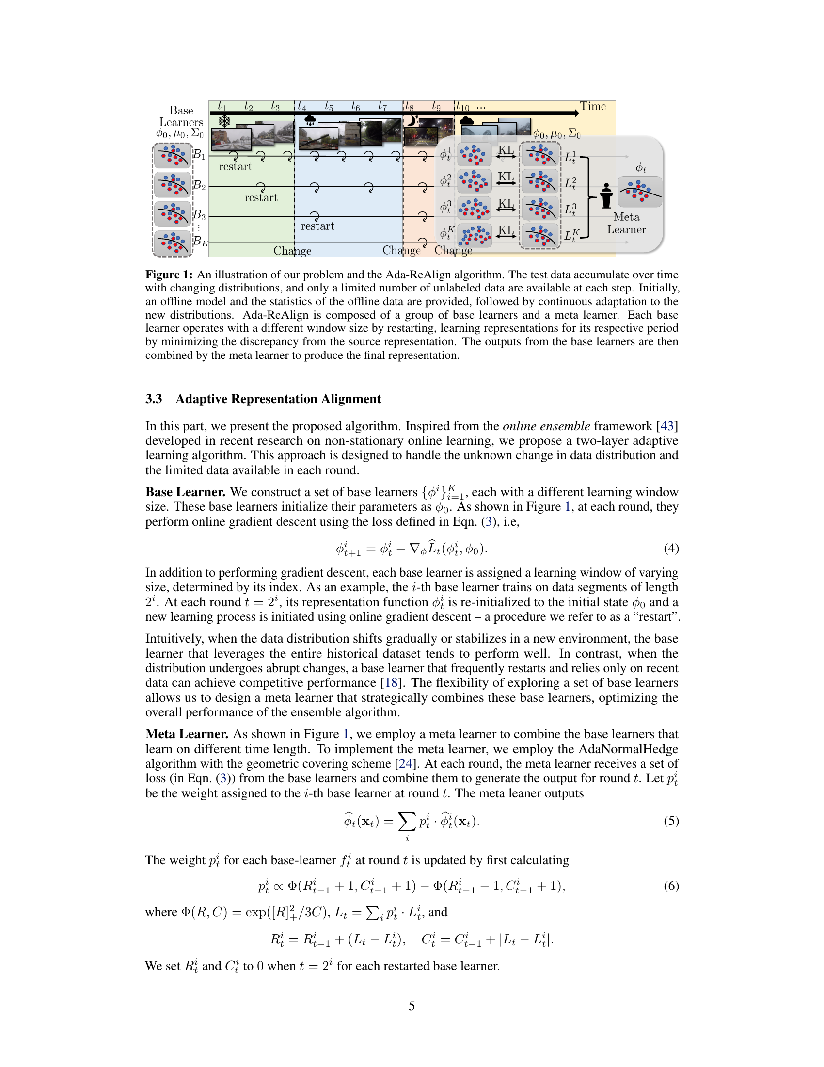
🔼 This figure illustrates the Ada-ReAlign algorithm, which addresses the challenge of continual test-time adaptation in non-stationary environments. The algorithm uses multiple base learners, each with a different window size, to process incoming unlabeled data. Each base learner updates its representation to align with the initial source domain representation. A meta-learner combines the outputs of these base learners to produce a final, adapted representation. The figure shows how the data distribution changes over time and the mechanism of restarting the base learners to adapt to these shifts.
read the caption
Figure 1: An illustration of our problem and the Ada-ReAlign algorithm. The test data accumulate over time with changing distributions, and only a limited number of unlabeled data are available at each step. Initially, an offline model and the statistics of the offline data are provided, followed by continuous adaptation to the new distributions. Ada-ReAlign is composed of a group of base learners and a meta learner. Each base learner operates with a different window size by restarting, learning representations for its respective period by minimizing the discrepancy from the source representation. The outputs from the base learners are then combined by the meta learner to produce the final representation.
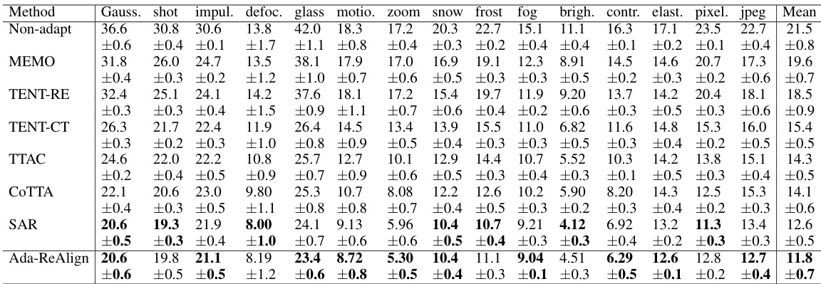
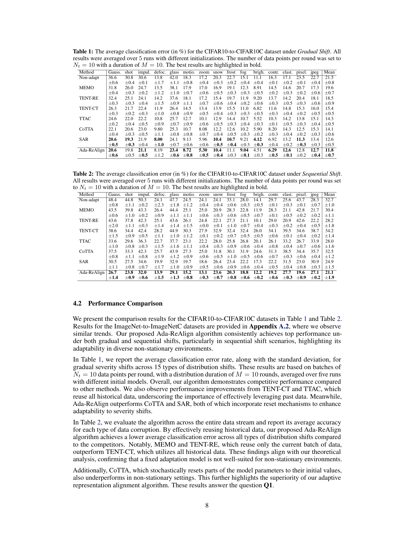
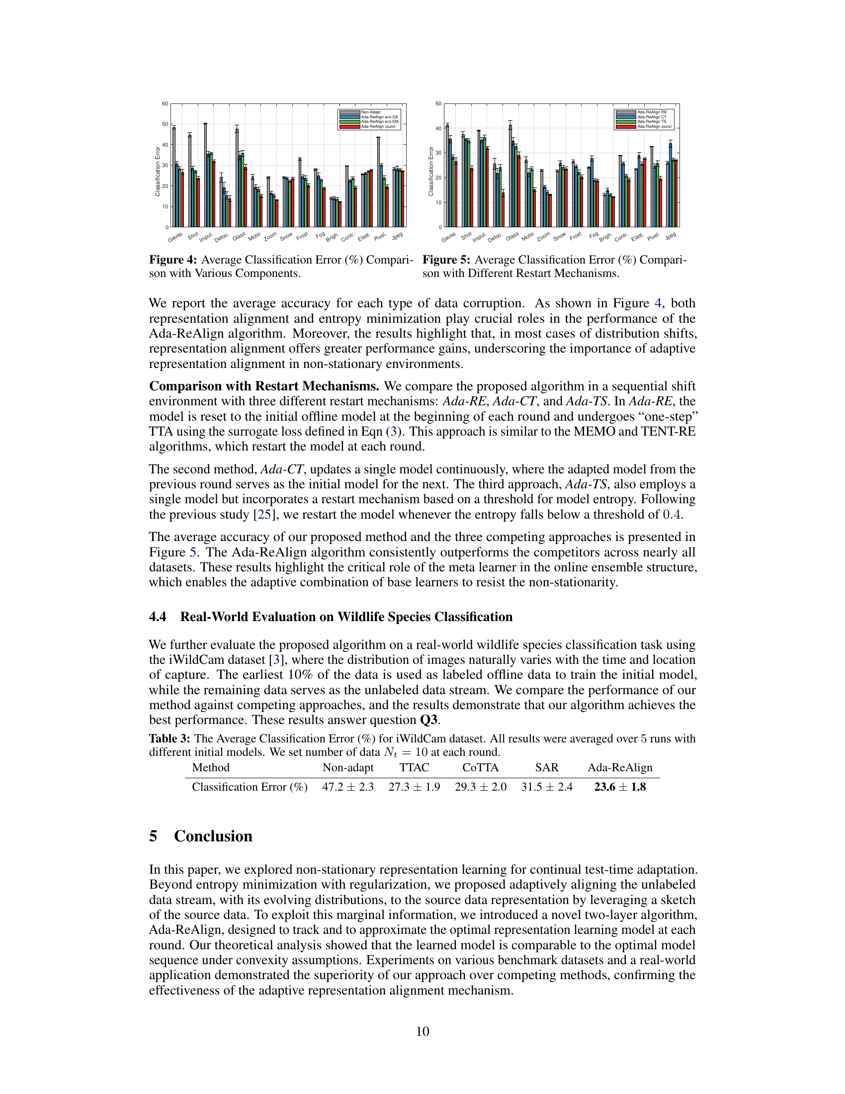
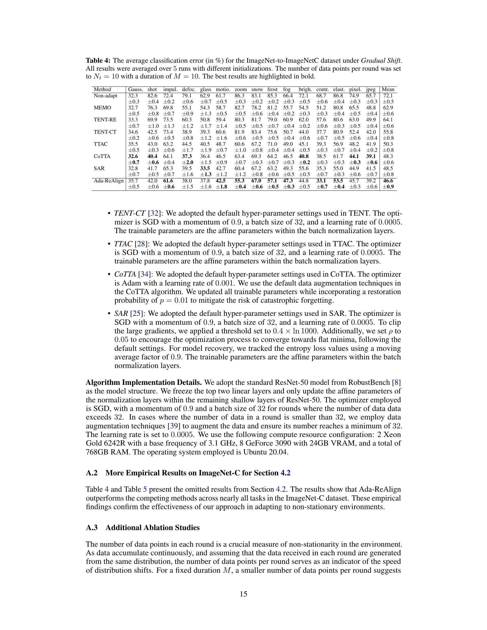
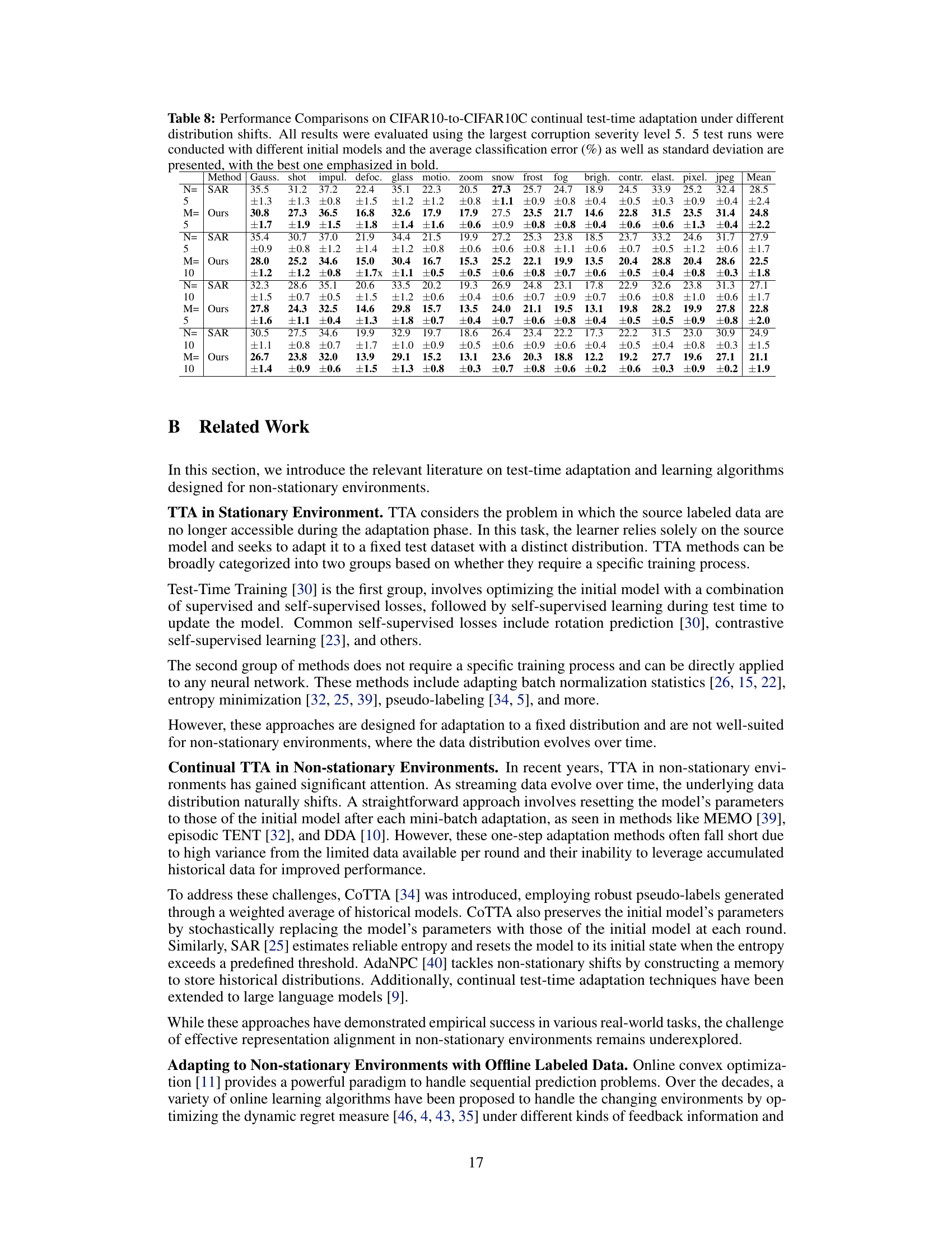
🔼 This table shows the average classification error rates for different corruption types in the CIFAR10C dataset under gradual shift conditions. The results are averaged over five runs with different model initializations, each using a batch size of 10 data points per round, and a duration of 10 rounds before a shift in corruption severity. The lowest error rate for each corruption type is highlighted in bold.
read the caption
Table 1: The average classification error (in %) for the CIFAR10-to-CIFAR10C dataset under Gradual Shift. All results were averaged over 5 runs with different initializations. The number of data points per round was set to Nt = 10 with a duration of M = 10. The best results are highlighted in bold.
In-depth insights#
Non-stationary TTA#
Non-stationary Test-Time Adaptation (TTA) tackles the challenge of adapting machine learning models to real-world scenarios where data distributions shift continuously. Unlike traditional TTA which assumes a fixed target distribution, non-stationary TTA must handle the dynamic nature of incoming data streams. This necessitates innovative approaches that go beyond simple model retraining or fine-tuning. Effective methods often leverage techniques such as online learning, enabling the model to adapt incrementally to each new batch of data. Pseudo-labeling, or using predictions as training data, plays a significant role, but requires careful consideration of uncertainty and label noise in the ever-changing environment. Representation alignment, ensuring the feature space of the unlabeled data aligns with that of the source domain, is another critical aspect, especially in non-stationary settings. Continual learning techniques are frequently integrated to facilitate ongoing adaptation without catastrophic forgetting. Ultimately, non-stationary TTA is a very active area of research that demands robust algorithms capable of learning and adapting continuously in dynamic and unpredictable environments.
Ada-ReAlign Algo#
The Ada-ReAlign algorithm is a novel approach to continual test-time adaptation in non-stationary environments. It cleverly addresses the challenge of limited unlabeled data and shifting distributions by employing an ensemble of base learners with varying window sizes. This approach allows exploration of different lengths of the data stream, offering adaptability to various shift patterns. The base learners’ outputs are then intelligently combined by a meta-learner, leading to robust performance. The algorithm’s design incorporates theoretical guarantees under convexity assumptions, offering a solid foundation. Experiments across benchmark datasets and real-world applications show Ada-ReAlign’s effectiveness in improving performance and adapting to unknown and continuously evolving data distributions. Key strengths include its ability to leverage source data’s marginal information for effective representation alignment and its efficient online learning mechanism, overcoming limitations of previous approaches. Further investigation is suggested to explore the algorithm’s adaptability in the presence of extremely high dimensional data, and its resilience in very noisy scenarios.
Source Data Sketch#
The concept of a “Source Data Sketch” in the context of test-time adaptation is intriguing. It suggests a method for model adaptation that avoids reliance on the full source dataset, addressing potential privacy, storage, or computational constraints. A sketch could involve summarizing key statistical properties of the source data (e.g., mean, covariance) or employing dimensionality reduction techniques to capture essential information concisely. This approach is particularly valuable in non-stationary environments where the target distribution changes dynamically, as it provides a stable reference point for alignment. Effective sketch design is crucial; it must capture enough information to guide adaptation accurately while remaining computationally efficient and resilient to noise or distribution drift. The effectiveness of a source data sketch hinges on the appropriate choice of summary statistics and their robustness against variations in the target domain. A well-designed sketch could potentially enhance the generalization performance and adaptability of the model, making it more robust to changes in the data distribution.
Ablation Experiments#
Ablation experiments systematically remove components of a model to assess their individual contributions. In a test-time adaptation (TTA) paper, this might involve removing different modules (e.g., representation alignment, entropy minimization), data augmentation strategies, or the meta-learner. By observing performance changes after each ablation, researchers can understand the relative importance of different components in the overall system. This provides crucial insights into the model’s architecture and the effectiveness of design choices. Well-designed ablation studies are essential for demonstrating the necessity of each component and avoiding spurious correlations. For instance, an ablation showing that removing representation alignment significantly harms performance supports the claim that it is a critical part of the model’s success and is not simply a helpful add-on. Conversely, if the ablation of a component leads to minimal performance degradation, it suggests its contribution is less significant than initially assumed, prompting a re-evaluation of design decisions. Such experiments validate model claims, and enhance the generalizability of the method. They help avoid overfitting to specific datasets or experimental setups, and provide a more robust understanding of how each piece of the model works to enable effective adaptation.
Real-world test#
A robust research paper should include a dedicated ‘Real-world test’ section to evaluate the practical applicability and effectiveness of the proposed methodology beyond simulated or benchmark datasets. This section should showcase how the algorithm performs under real-world conditions, which are often characterized by noisy data, uncertain environments, and evolving data distributions. It is crucial to demonstrate the algorithm’s adaptability and robustness when confronted with these real-world challenges. The experiments should be designed to mimic real-world scenarios as closely as possible. This might involve using diverse real-world datasets, conducting long-term studies to assess continual adaptation, and thoroughly analyzing the algorithm’s sensitivity to various parameters and operating conditions. A lack of real-world testing undermines the practical value and impact of the research, regardless of how promising the results look in controlled settings. Therefore, a comprehensive ‘Real-world test’ section is essential for establishing the trustworthiness and validity of the proposed approach.
More visual insights#
More on figures

🔼 This figure shows the weights assigned to each base learner in Ada-ReAlign across different time intervals (M) under sequential and Bernoulli shifts. Each heatmap visualizes the weight distribution across K base learners, where each learner has a different window size (2^i, i=0,…,K-1). The sequential shift shows a clear pattern: weights are concentrated on learners with window sizes matching the length of distribution stability (M). The Bernoulli shift shows a more diffuse weight distribution. The x-axis represents window size, while the y-axis represents time interval (M) length.
read the caption
Figure 2: Weight (%) heatmap of base learners in (a) Sequential shift with different intervals. (b) Bernoulli sequential shift with different intervals, where the length of interval is an expected value.

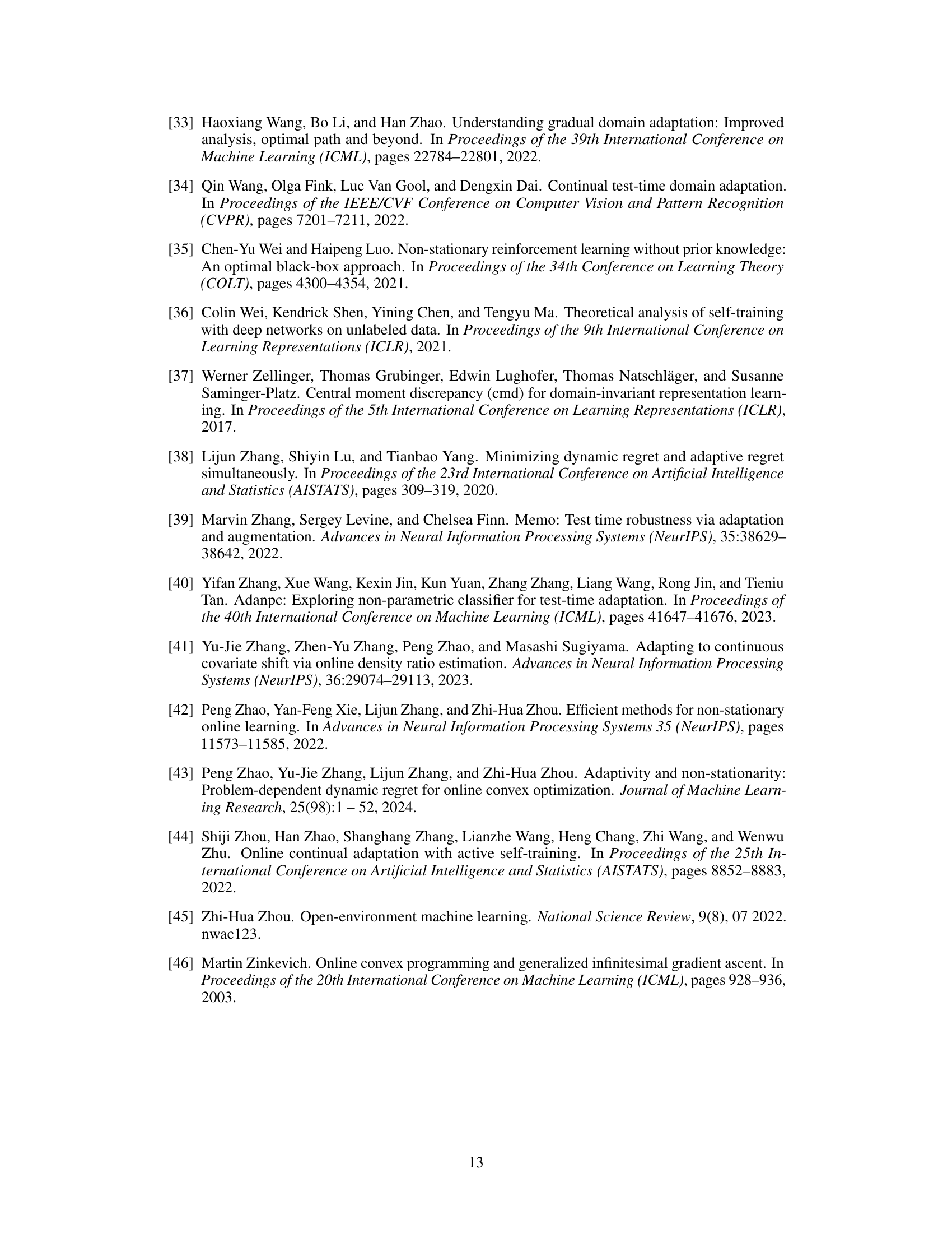
🔼 This figure compares the average classification error rates of different variants of the Ada-ReAlign algorithm across various corruption types in the CIFAR-10C dataset. The variants include Ada-ReAlign without distribution alignment (w/o DA), Ada-ReAlign with only representation alignment (RE), Ada-ReAlign with only entropy minimization (EM), Ada-ReAlign using the TENT algorithm’s restart mechanism (CT), and Ada-ReAlign using a threshold-based restart mechanism (TS). The results highlight the importance of both representation alignment and entropy minimization in achieving high performance. The standard error bars are also shown for each result.
read the caption
Figure 4: Average Classification Error (%) Comparison with Various Components.
More on tables
🔼 This table presents the average classification error rates for CIFAR10-to-CIFAR10C dataset under gradual shift conditions. The experiment was repeated 5 times with different initializations, using 10 data points per round and a duration of 10 rounds per distribution. The lowest error rates are highlighted in bold, showing the relative performance of various algorithms.
read the caption
Table 1: The average classification error (in %) for the CIFAR10-to-CIFAR10C dataset under Gradual Shift. All results were averaged over 5 runs with different initializations. The number of data points per round was set to Nt = 10 with a duration of M = 10. The best results are highlighted in bold.

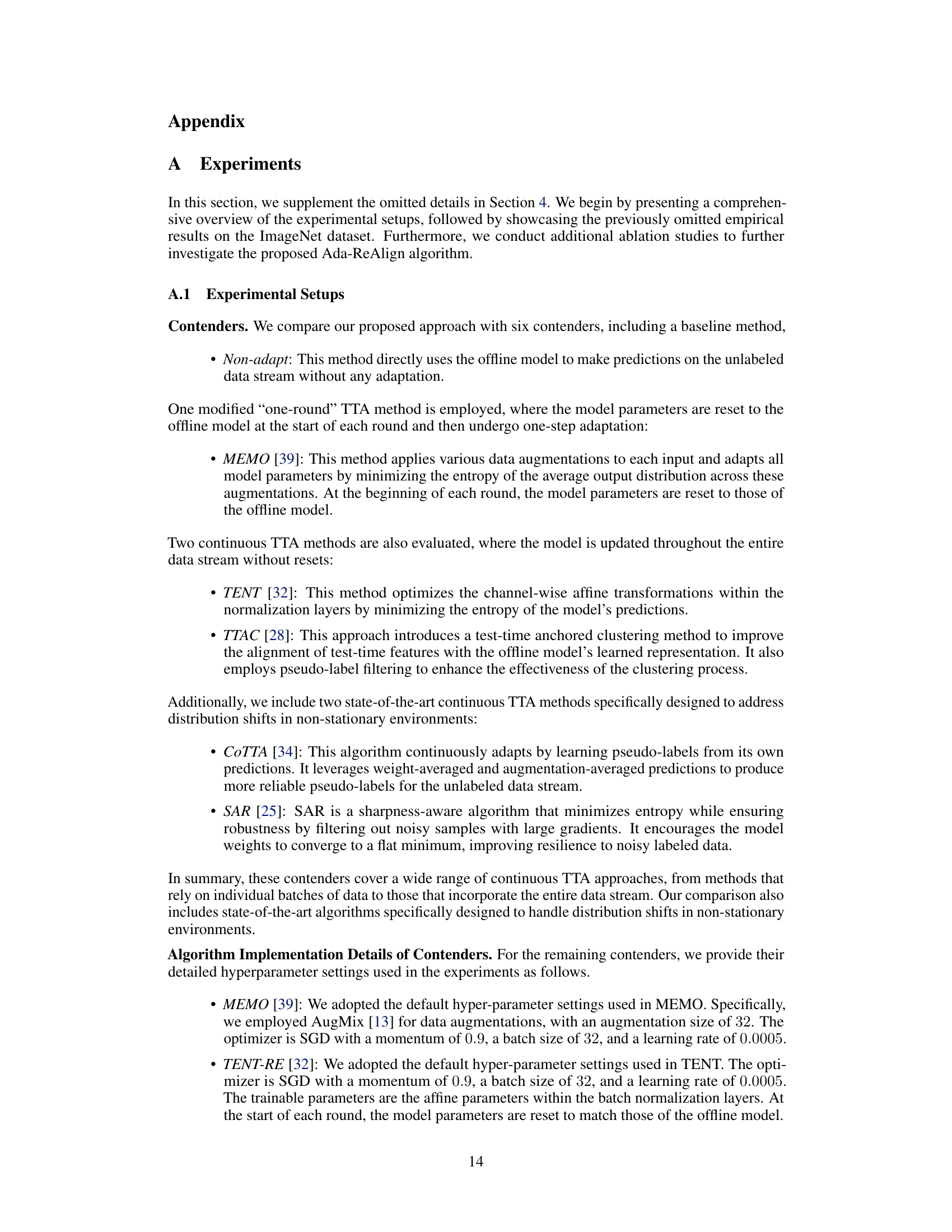
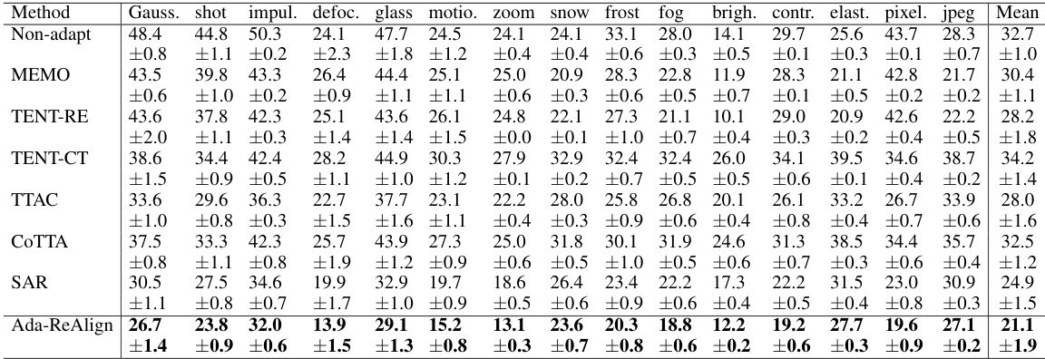
🔼 This table presents the average classification error rates achieved by different methods on the iWildCam dataset for a real-world wildlife species classification task. The results highlight the performance of the proposed Ada-ReAlign algorithm compared to existing methods in a real-world, non-stationary environment where the distribution of data naturally varies over time and location.
read the caption
Table 3: The Average Classification Error (%) for iWildCam dataset. All results were averaged over 5 runs with different initial models. We set number of data Nt = 10 at each round.

🔼 This table presents the average classification error rates for CIFAR10-to-CIFAR10C dataset under gradual shift conditions. The results are obtained by averaging over 5 runs with different initializations. The number of data points used per round (Nt) is 10, and the duration for which the data distribution remains unchanged (M) is also 10. The best performing methods for each corruption type are highlighted in bold.
read the caption
Table 1: The average classification error (in %) for the CIFAR10-to-CIFAR10C dataset under Gradual Shift. All results were averaged over 5 runs with different initializations. The number of data points per round was set to Nt = 10 with a duration of M = 10. The best results are highlighted in bold.

🔼 This table presents the average classification error rates for the CIFAR10-to-CIFAR10C dataset under a gradual shift in data distribution. The results are broken down by type of image corruption (Gaussian noise, shot noise, impulse noise, defocus blur, glass blur, motion blur, zoom blur, snow, frost, fog, brightness, contrast, elastic transform, pixelate, JPEG compression) and averaged across five runs with different random initializations. Each run uses batches of 10 data points and a duration of 10 rounds (M=10) between shifts in distribution severity. The lowest error rate for each corruption type is highlighted in bold.
read the caption
Table 1: The average classification error (in %) for the CIFAR10-to-CIFAR10C dataset under Gradual Shift. All results were averaged over 5 runs with different initializations. The number of data points per round was set to Nt = 10 with a duration of M = 10. The best results are highlighted in bold.

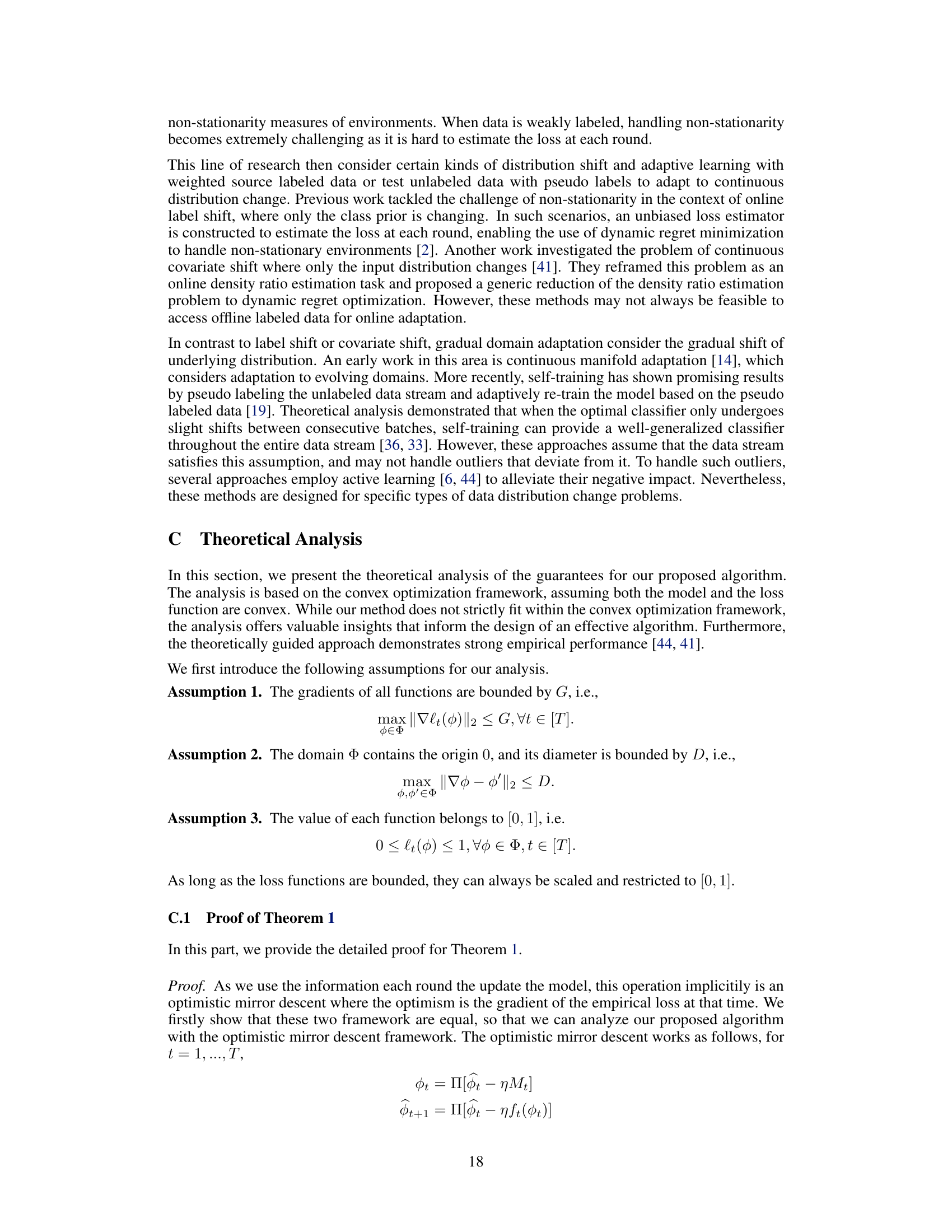
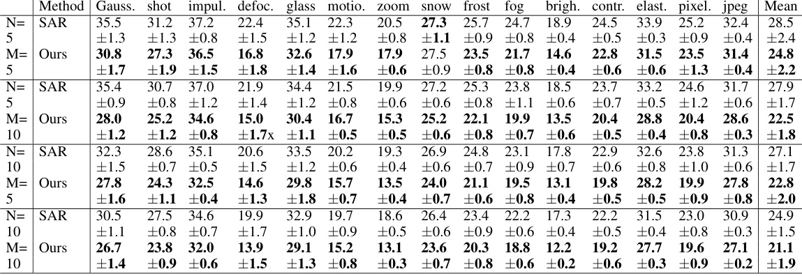
🔼 This table shows the average classification error rates for the CIFAR10-to-CIFAR10C dataset under a sequential shift in data distribution. The experiment used the highest corruption severity level (5) and ran 5 times with different initial model parameters. The number of data points per round (Nt) was varied while maintaining a duration of 10 rounds (M=10) for each distribution. The results demonstrate how the Ada-ReAlign algorithm’s performance changes with different amounts of data available during each adaptation step.
read the caption
Table 6: The Average Classification Error (%) for CIFAR10-to-CIFAR10C Dataset under Sequential Shift. All results were evaluated using the largest corruption severity level 5 and averaged over 5 runs with different initial models. We set different number of data Nt at each round with duration M = 10.
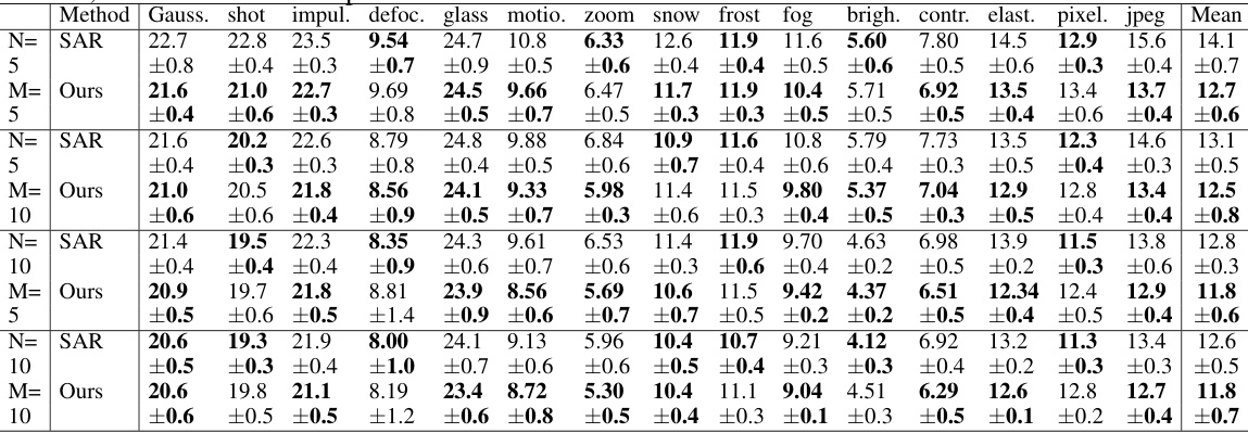
🔼 This table presents the average classification error rates for CIFAR-10C dataset under gradual shift conditions. The experiment was repeated 5 times with different random initializations. Each round consisted of 10 data points and the data distribution remained unchanged for 10 rounds. The lowest error rate for each corruption type is shown in bold.
read the caption
Table 1: The average classification error (in %) for the CIFAR10-to-CIFAR10C dataset under Gradual Shift. All results were averaged over 5 runs with different initializations. The number of data points per round was set to Nt = 10 with a duration of M = 10. The best results are highlighted in bold.
🔼 This table presents the average classification error rates for CIFAR-10 to CIFAR-10C dataset under gradual distribution shifts. The results are obtained by averaging over five runs with different initializations. The number of data points used in each round is 10, and the duration of a distribution is 10 rounds. The best-performing models are highlighted in bold.
read the caption
Table 1: The average classification error (in %) for the CIFAR10-to-CIFAR10C dataset under Gradual Shift. All results were averaged over 5 runs with different initializations. The number of data points per round was set to Nt = 10 with a duration of M = 10. The best results are highlighted in bold.
Full paper#
