TL;DR#
Distributed deep learning faces a major challenge: high communication costs between servers and clients, especially for large models. Randomized sketching reduces this cost but existing theoretical analyses had limitations, either depending heavily on model size or requiring restrictive assumptions like heavy-hitter model updates. These pessimistic analyses contradict empirical evidence showing sketching’s effectiveness.
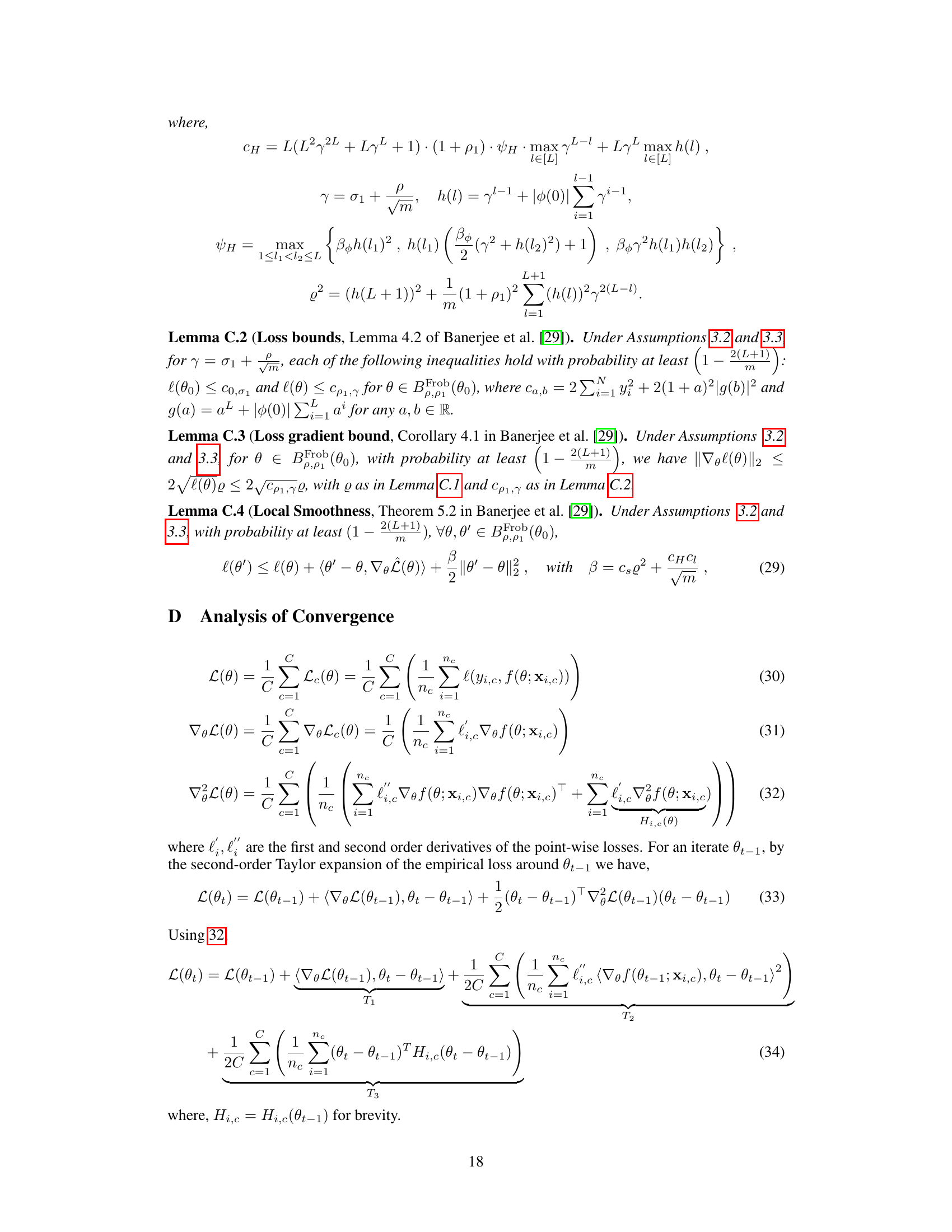
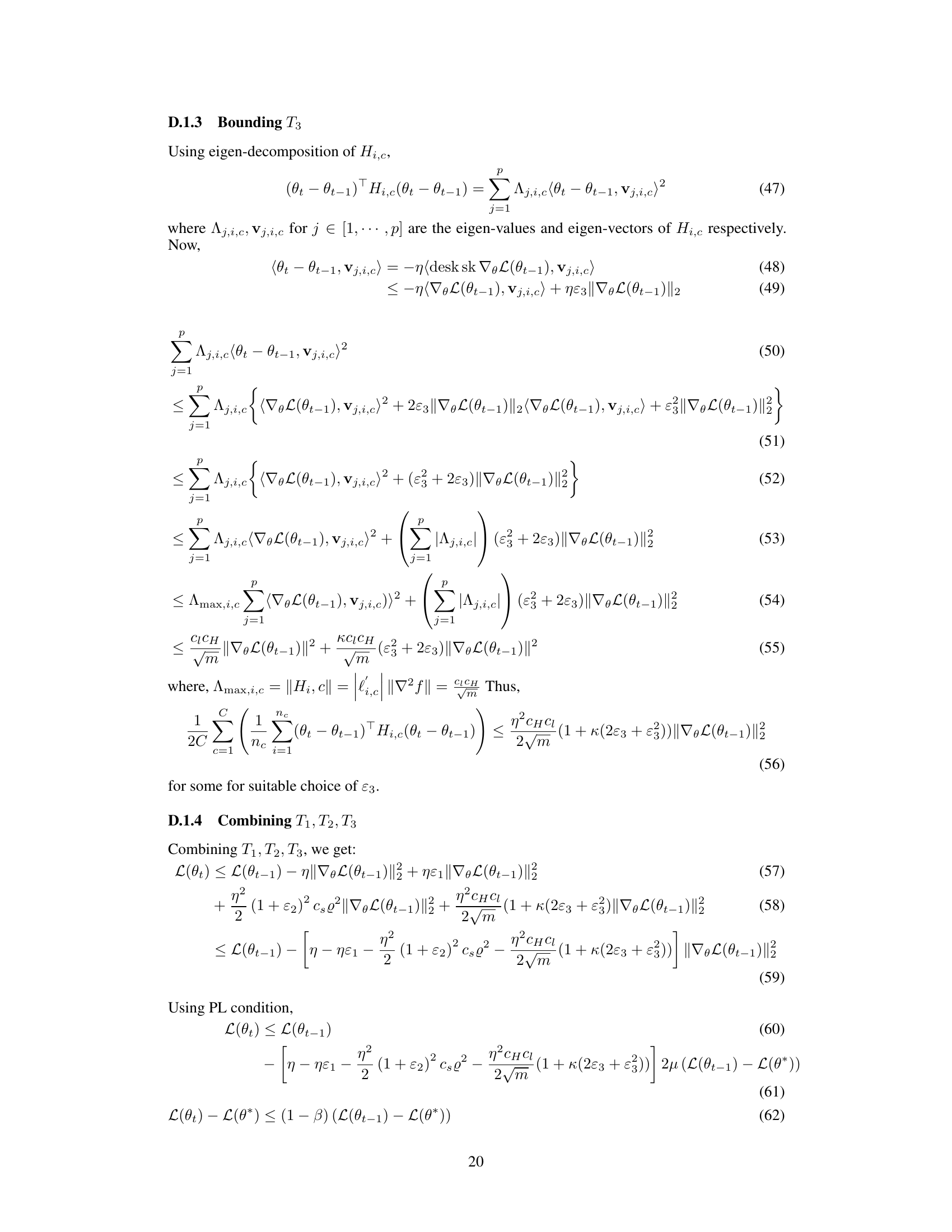
This paper introduces a sharper analysis for sketching-based distributed learning, using second-order geometry of the loss function to prove convergence results. This new approach eliminates the problematic dependence on ambient dimension in convergence error without making additional assumptions. The paper provides both theoretical and empirical results supporting these findings, finally offering a theoretical justification for sketching’s practical success and highlighting the ambient dimension-independent communication complexity.
Key Takeaways#
Why does it matter?#
This paper is crucial because it addresses the significant communication bottleneck in distributed deep learning, a major hurdle in scaling up these models. By providing a sharper analysis and eliminating the ambient dimension dependence, it justifies the empirical success of sketching-based methods and opens new avenues for creating more efficient and scalable distributed learning algorithms. Its focus on the second-order geometry of loss functions offers a novel perspective that can guide future research in this area.
Visual Insights#

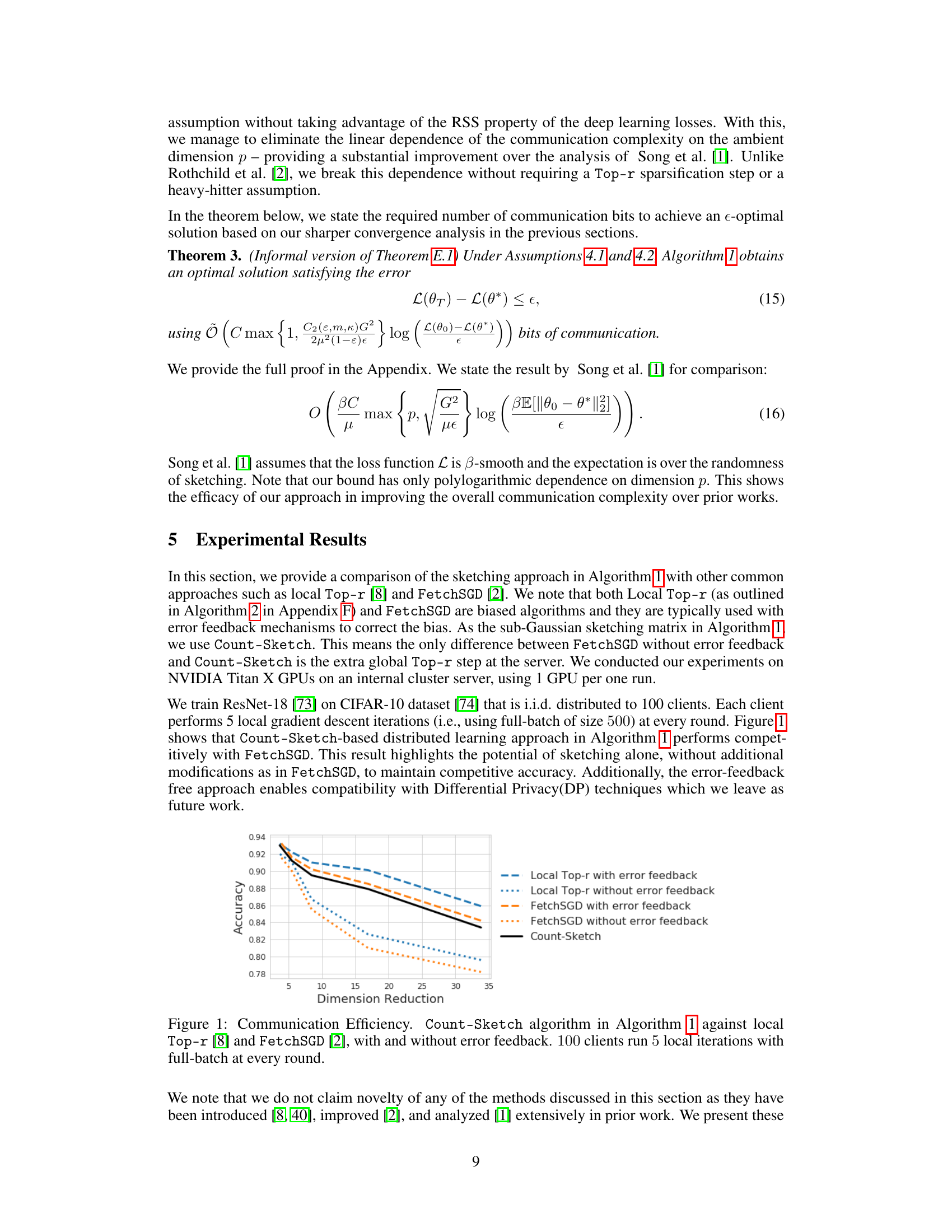
🔼 The figure compares the communication efficiency of the Count-Sketch algorithm proposed in the paper against two other common approaches, Local Top-r and FetchSGD, both with and without error feedback mechanisms. The experiment used 100 clients, each performing 5 local iterations using full batches of data in every round. The x-axis represents the degree of dimension reduction, and the y-axis shows the accuracy achieved. The results demonstrate that Count-Sketch achieves competitive accuracy even without error feedback.
read the caption
Figure 1: Communication Efficiency. Count-Sketch algorithm in Algorithm 1 against local Top-r [8] and FetchSGD [2], with and without error feedback. 100 clients run 5 local iterations with full-batch at every round.

🔼 This table compares the iteration complexities and assumptions of the proposed sketching method with those of prior works, specifically Song et al. [1]. It highlights the ambient dimension independence achieved by the proposed method under the assumption of Polyak-Łojasiewicz (PL) condition and approximate restricted strong smoothness (RSS). In contrast, prior work exhibits a dependence on the ambient dimension under the assumption of strong convexity and β-smoothness. The table also defines constant values used in the analysis.
read the caption
Table 1: Comparison of iteration complexities and assumptions with prior work. Cs, CĮ are constants defined in Assumption 3.2 and Q, CH are defined in Lemma C.1,Lemma C.2 respectively. Note that o and CH are O(poly(L)) and can be seen as independent of ambient dimension for wide networks. Under our assumptions and setup (Section 3). According to Lemma C.4 the loss function L can be shown to be B-smooth where β = O(p² + m). SC refers to strong-convexity and PL refers to PL-condition.
In-depth insights#
Sketch-DL Analysis#
The analysis of Sketch-DL, or sketching-based distributed deep learning, reveals critical insights into communication efficiency. Existing analyses often suffered from a strong dependence on the ambient model dimension, hindering scalability. This sharper analysis leverages the second-order geometry of the loss function, specifically using the approximate restricted strong smoothness (RSS) property of deep models. This approach provides dimension-independent convergence bounds, overcoming the limitations of prior work. The improved theoretical understanding is supported by empirical evidence demonstrating competitive performance compared to uncompressed methods. Avoiding restrictive assumptions, like the heavy-hitter assumption, makes the Sketch-DL approach more broadly applicable. The results highlight the value of RSS in analyzing Sketch-DL and its potential for achieving significant communication savings in large-scale distributed training.
RSS in Sketch-DL#
The concept of “RSS in Sketch-DL” suggests exploring the implications of Restricted Strong Smoothness (RSS) within the framework of sketching for distributed deep learning. RSS acknowledges that deep learning loss functions exhibit strong smoothness only in specific directions, unlike the traditional assumption of global smoothness. This characteristic is crucial because sketching inherently involves projecting high-dimensional data into lower dimensions, potentially affecting the optimization landscape. A sharper analysis using RSS could reveal dimension-independent convergence guarantees for sketch-DL, overcoming limitations of prior analyses that relied on global smoothness assumptions and suffered from dependence on ambient dimension. By incorporating RSS, we can potentially explain the empirical success of sketching despite its pessimistic theoretical bounds, paving the way for more efficient and scalable distributed deep learning algorithms. Exploiting RSS offers the potential to refine the communication complexity bounds of sketch-DL, demonstrating that sketching’s advantages are not negated by the high-dimensionality of modern deep models. This is achieved by focusing on the geometric properties of the loss function in restricted directions rather than relying on overall smoothness.
Dimensionality Issue#
High-dimensional data is a pervasive challenge in machine learning, and distributed deep learning is no exception. The ‘dimensionality issue’ refers to the computational and communication burdens associated with transmitting and processing massive model parameters in a distributed setting. Existing theoretical analyses of sketching-based distributed learning (sketch-DL) often suffer from a prohibitive dependence on the ambient dimension, leading to pessimistic results that don’t align with empirical success. This discrepancy highlights a critical need for improved analysis. A sharper analysis might leverage the geometry of the loss function, specifically exploiting the approximate restricted strong smoothness (RSS) property observed in overparameterized deep models. By focusing on second-order properties of the loss Hessian rather than relying solely on global smoothness assumptions, it may be possible to derive ambient dimension-independent convergence guarantees for sketch-DL. This would demonstrate that the empirical competitiveness of sketch-DL is not merely coincidental but rather a consequence of inherent properties of the models and optimization techniques employed. The key to unlocking more optimistic results likely lies in a more nuanced understanding of the high-dimensional geometry and a move beyond simplistic smoothness assumptions.
Communication Cost#
In distributed deep learning, communication cost is a major bottleneck, especially when dealing with large models. The paper focuses on reducing this cost through sketching, a technique that compresses model updates before transmission between clients and servers. Existing analysis often suffers from a dependence on ambient dimension, leading to pessimistic results. This work provides a sharper analysis, showing that sketching achieves ambient dimension-independent convergence, justified by the use of second-order geometry of the loss function and avoiding global smoothness assumptions. The results support the empirical success of sketching and demonstrate that it is a viable communication-efficient strategy. This approach allows for a substantial reduction in communication overhead, paving the way for improved scalability and efficiency in distributed deep learning.
Future of Sketch-DL#
The future of Sketch-DL (Sketching for Distributed Deep Learning) is promising, particularly given its demonstrated ability to mitigate communication bottlenecks in large-scale training. Further research should focus on refining the theoretical understanding of Sketch-DL, moving beyond current limitations like restrictive assumptions and dimension dependence. Exploring new sketching techniques tailored for specific deep learning architectures and loss functions could drastically improve efficiency and accuracy. Combining Sketch-DL with other compression methods like quantization or sparsification could offer synergistic benefits, creating highly efficient hybrid approaches. Investigating Sketch-DL’s compatibility with advanced optimization algorithms and privacy-preserving techniques is crucial for expanding its real-world applicability. Empirical evaluations on diverse datasets and deep learning models are vital to validating theoretical advancements and establishing Sketch-DL’s robustness. Finally, developing standardized benchmarks and evaluation metrics will enhance reproducibility and facilitate meaningful comparisons between different Sketch-DL variants.
More visual insights#
More on figures

🔼 This figure shows the value of κ (kappa) across training epochs for two different loss functions: Binary Cross Entropy (BCE) and Mean Squared Error (MSE). Kappa is defined as the sum of absolute eigenvalues divided by the maximum eigenvalue of the predictor Hessian. The plot shows how this value changes as the model trains, indicating the evolution of the second-order properties of the loss function over time. This is relevant to the paper’s analysis because it helps demonstrate that the restricted strong smoothness (RSS) property, which is crucial to their theoretical findings, holds in practice. The relatively small values of κ compared to the model dimension support their core argument that the ambient dimension does not hinder the performance of sketching-based distributed learning.
read the caption
Figure 24: Estimate of κ = Σi=1 |λi|/λmax over training iterations.

🔼 This figure shows the spectral density of the predictor Hessian for a ResNet-18 model trained on 1000 samples from the CIFAR-10 dataset, at different training epochs (500, 1000, and 1500). The spectral density is calculated using the Binary Cross Entropy loss function. The plots visualize the distribution of eigenvalues of the Hessian, showing a concentration of eigenvalues around zero and a rapid decay in density as eigenvalues move away from zero. This demonstrates the restricted strong convexity of the loss function, a key property used in the paper’s analysis.
read the caption
Figure 3: Spectral Density of Predictor Hessian :H(θ, x₁) = l'i∇²f(θ; x₁) for a fixed training input across training epochs. Dataset : 1000 samples from CIFAR-10 dataset. Model: ResNet-18. The model has 1.1 × 10⁷ parameters. Loss function: Binary Cross Entropy(BCE) Loss.
🔼 The figure shows the estimate of kappa (κ) which is the sum of absolute eigenvalues of the predictor Hessian (H) divided by the maximum eigenvalue (λmax) for a fixed training input across training epochs. The data is from 1000 samples of the CIFAR-10 dataset, using a ResNet-18 model with approximately 11 million parameters and the Binary Cross Entropy loss function.
read the caption
Figure 2: Estimate of k = Σ=1 |λi|/λmax of H₁ for a fixed training input across training epochs. Dataset: 1000 samples from CIFAR-10 dataset. Model: ResNet-18. The model has 1.1 × 10⁷ parameters. Loss function: Binary Cross Entropy(BCE) Loss.
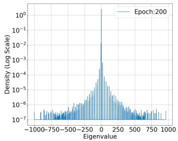
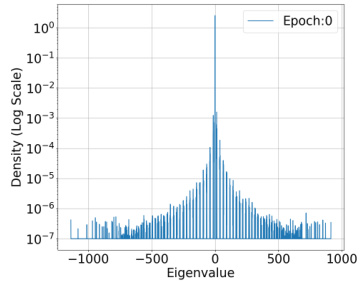
🔼 This figure shows the spectral density of the predictor Hessian for a fixed training input at different training epochs. The dataset used is CIFAR-10, the model is ResNet-18, and the loss function is Binary Cross Entropy. The plot visualizes the distribution of eigenvalues of the Hessian matrix, which provides insights into the model’s curvature and how it changes during training. The density is shown on a log scale.
read the caption
Figure 5: Spectral Density of Predictor Hessian :H(θ, x₁) = l'i∇²f(θ; x₁) for a fixed training input across training epochs. Dataset: 1000 samples from CIFAR-10 dataset. Model: ResNet-18. The model has 1.1 × 10⁷ parameters. Loss function: Binary Cross Entropy(BCE) Loss.

🔼 This figure shows the spectral density of the predictor Hessian for a fixed training input across multiple training epochs. The data is from the CIFAR-10 dataset, and a ResNet-18 model (with approximately 11 million parameters) and binary cross-entropy loss function were used. The plot shows the distribution of eigenvalues of the Hessian, illustrating the concentration of eigenvalues around zero and the rapid decay of the density for larger eigenvalues.
read the caption
Figure 6: Spectral Density of Predictor Hessian :H(θ, x₁) = l'i∇²f(θ; x₁) for a fixed training input across training epochs. Dataset: 1000 samples from CIFAR-10 dataset. Model: ResNet-18. The model has 1.1 × 10⁷ parameters. Loss function: Binary Cross Entropy(BCE) Loss.

🔼 This figure shows the spectral density of the predictor Hessian H(θ,x) = l’i∇²f(θ;x) for a fixed training input at epoch 600. The dataset used is CIFAR-10, and the model is ResNet-18 with 1.1 × 10⁷ parameters. The loss function is Binary Cross Entropy (BCE) Loss. The figure illustrates the distribution of eigenvalues of the Hessian matrix, highlighting the concentration of eigenvalues around zero, which is consistent with the RSS property discussed in the paper.
read the caption
Figure 7: Epoch: 600

🔼 This figure shows the spectral density of the predictor Hessian for a fixed training input at different training epochs (epoch 800 is shown here). It uses the ResNet-18 model trained on 1000 samples from the CIFAR-10 dataset with binary cross-entropy loss. The x-axis represents the eigenvalues, and the y-axis represents the density (log scale). This visualization helps to understand the distribution of eigenvalues of the Hessian, which is relevant to the paper’s analysis of the restricted strong smoothness property of deep learning losses.
read the caption
Figure 8: Spectral Density of Predictor Hessian :H(0, x₁) = l'¿∇²f(0; x₁) for a fixed training input across training epochs. Dataset: 1000 samples from CIFAR-10 dataset. Model: ResNet-18. The model has 1.1 × 10⁷ parameters. Loss function: Binary Cross Entropy(BCE) Loss.
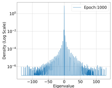
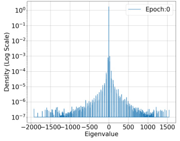
🔼 This figure shows the spectral density of the predictor Hessian for a ResNet-18 model trained on 1000 samples from the CIFAR-10 dataset, using the binary cross-entropy loss function. The spectral density is computed for a fixed training input across multiple training epochs (500, 1000, and 1500). The figure helps to visualize how the eigenvalues of the Hessian change during the training process, providing insights into the optimization landscape and the model’s learning dynamics.
read the caption
Figure 3: Spectral Density of Predictor Hessian :H(0, x₁) = l'¿∇²f(0; x₁) for a fixed training input across training epochs. Dataset : 1000 samples from CIFAR-10 dataset. Model: ResNet-18. The model has 1.1 × 10⁷ parameters. Loss function: Binary Cross Entropy(BCE) Loss.

🔼 This figure is one of a set of figures (Figure 10-Figure 12 and Figure 14-Figure 22) showing the spectral density of the predictor Hessian H(θ, x₁) = l’i∇²f(θ; x₁) for a fixed training input across multiple training epochs. The model used is ResNet-18 with 1.1 × 10⁷ parameters. Two loss functions are used: Binary Cross Entropy (BCE) and Mean Squared Error (MSE). Each figure shows the density distribution of eigenvalues. The data used is 1000 samples from the CIFAR-10 dataset. These figures support the authors’ analysis and observations regarding the properties of the loss function in deep learning models.
read the caption
Figure 10: Epoch: 1200

🔼 This figure shows the spectral density of the predictor Hessian for a fixed training input at epoch 1400. The dataset used is 1000 samples from CIFAR-10, the model is ResNet-18 (with 11 million parameters), and the loss function is Binary Cross Entropy (BCE) Loss. The graph displays the density (in log scale) on the y-axis and the eigenvalue on the x-axis. It shows a distribution of eigenvalues, concentrating near zero, suggesting that the Hessian’s spectrum displays a bulk and outliers structure, with most of the eigenvalues having very small values.
read the caption
Figure 11: Epoch: 1400

🔼 This figure shows the spectral density of the predictor Hessian for a ResNet-18 model trained on 1000 samples from the CIFAR-10 dataset using the mean squared error loss function. The spectral density is calculated for a fixed training input across multiple training epochs. The figure is intended to visually support the claim that the sum of absolute eigenvalues of the predictor Hessian is bounded (Assumption 4.2).
read the caption
Figure 23: Spectral Density of Predictor Hessian :H(0, x₁) = l'¿∇²f(0; x₁) for a fixed training input across training epochs. Dataset: 1000 samples from CIFAR-10 dataset. Model: ResNet-18. The model has 1.1 × 10⁷ parameters. Loss function: Mean Squared Error (MSE).
🔼 This figure shows the estimate of the constant kappa (κ) across training epochs. Kappa is calculated as the sum of absolute eigenvalues divided by the maximum eigenvalue of the Hessian matrix of the predictor. The experiment used 1000 samples from the CIFAR-10 dataset, a ResNet-18 model, and binary cross-entropy loss. The results demonstrate that κ remains significantly smaller than the model dimension (p) throughout training, supporting Assumption 4.2 of the paper.
read the caption
Figure 2: Estimate of k = Σi=1 |λi|/λmax of H₁ for a fixed training input across training epochs. Dataset: 1000 samples from CIFAR-10 dataset. Model: ResNet-18. The model has 1.1 × 10⁷ parameters. Loss function: Binary Cross Entropy(BCE) Loss.
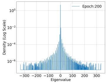
🔼 This figure shows the spectral density of the predictor Hessian across training epochs for a fixed training input using the BCE loss function. The dataset is CIFAR-10, and the model is ResNet-18. The plot shows that most eigenvalues of the Hessian are very close to zero with a quick decay away from zero.
read the caption
Figure 3: Spectral Density of Predictor Hessian :H(0, x₁) = l'i∇²f(0; x₁) for a fixed training input across training epochs. Dataset : 1000 samples from CIFAR-10 dataset. Model: ResNet-18. The model has 1.1 × 10⁷ parameters. Loss function: Binary Cross Entropy(BCE) Loss.

🔼 The figure compares the communication efficiency of three different distributed learning algorithms: Count-Sketch (Algorithm 1 from the paper), Local Top-r, and FetchSGD. It shows the accuracy achieved by each algorithm with varying degrees of dimension reduction. The experiment uses 100 clients performing 5 local full-batch gradient descent iterations per round. Notably, the comparison includes versions of Local Top-r and FetchSGD both with and without error feedback mechanisms, highlighting the impact of unbiased sketching in Count-Sketch.
read the caption
Figure 1: Communication Efficiency. Count-Sketch algorithm in Algorithm 1 against local Top-r [8] and FetchSGD [2], with and without error feedback. 100 clients run 5 local iterations with full-batch at every round.
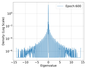
🔼 This figure shows the spectral density of the predictor Hessian for a fixed training input at epoch 600. The dataset used is CIFAR-10, the model is ResNet-18, and the loss function is Binary Cross Entropy (BCE). The x-axis represents the eigenvalues, and the y-axis shows the density (on a log scale). The plot visually demonstrates the distribution of eigenvalues, highlighting the concentration around zero and a rapid decay in density as the eigenvalues move away from zero. This observation is crucial to the paper’s argument about the restricted strong smoothness property of deep learning losses.
read the caption
Figure 7: Epoch: 600

🔼 This figure is one of a series of figures (Figure 7-Figure 9) showing the spectral density of the predictor Hessian across various training epochs. The x-axis represents the eigenvalues, and the y-axis represents the density (on a log scale). The data is from the CIFAR-10 dataset, using a ResNet-18 model with Binary Cross-Entropy loss. Each figure in the sequence shows the distribution of eigenvalues at a different training epoch (Epoch: 800 in this specific figure). This visualization is used to illustrate the distribution of eigenvalues of the predictor Hessian, which is relevant to the paper’s analysis of the restricted strong smoothness (RSS) property of deep learning models.
read the caption
Figure 8: Epoch: 800

🔼 This figure shows the spectral density of the predictor Hessian for a ResNet-18 model trained on 1000 samples from the CIFAR-10 dataset. The spectral density is computed using stochastic Lanczos quadrature for three different training epochs (500, 1000, and 1500). The figure illustrates that most of the eigenvalues of the Hessian are near zero, with a rapid decay in density as the magnitude of the eigenvalue increases. This observation supports the assumption of restricted strong smoothness, crucial for the paper’s analysis.
read the caption
Figure 3: Spectral Density of Predictor Hessian :H(θ, x₁) = l'i∇²f(θ; x₁) for a fixed training input across training epochs. Dataset : 1000 samples from CIFAR-10 dataset. Model: ResNet-18. The model has 1.1 × 10⁷ parameters. Loss function: Binary Cross Entropy(BCE) Loss.
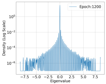
🔼 This figure shows the spectral density of the predictor Hessian for a fixed training input at epoch 1200. The dataset used is CIFAR-10 with 1000 samples, the model is ResNet-18, and the loss function is Binary Cross Entropy (BCE). The x-axis shows the eigenvalue, and the y-axis shows the density on a logarithmic scale. The plot illustrates the distribution of eigenvalues of the Hessian matrix, highlighting the concentration of eigenvalues around zero, which is a key observation supporting the paper’s theoretical analysis about the restricted strong smoothness property of deep learning losses.
read the caption
Figure 10: Epoch: 1200

🔼 This figure shows the spectral density of the predictor Hessian H(θ,x) = l’i∇²f(θ;x) for a fixed training input across training epochs. The dataset used is 1000 samples from the CIFAR-10 dataset. The model used is ResNet-18, which has 1.1 x 10⁷ parameters. The loss function is Mean Squared Error (MSE). The figure visually represents the distribution of eigenvalues of the Hessian matrix at epoch 1400 of training. It illustrates the concentration of eigenvalues around zero and the sparsity of the Hessian in this model.
read the caption
Figure 11: Epoch: 1400

🔼 The figure shows the spectral density of the predictor Hessian for a fixed training input across different training epochs. The dataset used is CIFAR-10, with a ResNet-18 model having 11 million parameters. The loss function employed is the Mean Squared Error (MSE). It illustrates the distribution of eigenvalues of the Hessian matrix, providing insights into the model’s optimization landscape during training.
read the caption
Figure 23: Spectral Density of Predictor Hessian :H(0, x₁) = l'i∇²f(0; x₁) for a fixed training input across training epochs. Dataset: 1000 samples from CIFAR-10 dataset. Model: ResNet-18. The model has 1.1 × 10⁷ parameters. Loss function: Mean Squared Error (MSE).
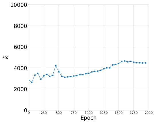
🔼 This figure shows the estimate of kappa (κ) which is the sum of absolute eigenvalues divided by the maximum eigenvalue of the Hessian across training iterations. The plot shows how this value changes over the training process for both Binary Cross Entropy (BCE) and Mean Squared Error (MSE) loss functions. The value of kappa is related to the restricted strong smoothness property of the loss function which is critical to the paper’s theoretical analysis.
read the caption
Figure 24: Estimate of k = ∑i=1 |λi|/λmax over training iterations.
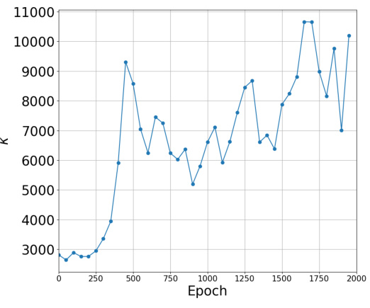
🔼 This figure shows the estimate of kappa (κ) across training iterations. Kappa is calculated as the sum of the absolute values of eigenvalues (λi) divided by the maximum eigenvalue (λmax) of the predictor Hessian. The plot illustrates how this value changes over time during the training process for two different loss functions: Binary Cross Entropy (BCE) and Mean Squared Error (MSE). The x-axis represents the training epoch, and the y-axis represents the value of κ.
read the caption
Figure 24: Estimate of κ = Σpi=1 |λi|/λmax over training iterations.
Full paper#

