TL;DR#
Current large vision models, while successful in 2D tasks, are not fully evaluated for their understanding of 3D physical properties like geometry, material, or lighting. Existing methods lack a generalized way to assess these capabilities, hindering progress in creating computer vision systems that truly understand the physical world. This makes it difficult to design models that accurately predict interactions between objects or respond to dynamic scenes.
This research introduces a general and efficient protocol to evaluate the models’ understanding of 3D physical properties. The method involves training classifiers on model features for different properties, allowing for a systematic and quantitative assessment. The study finds that Stable Diffusion and DINOv2 models perform best for many properties, suggesting architectural choices leading to better 3D understanding. The findings highlight opportunities for enhancing model design to improve 3D physical awareness, unlocking new applications for computer vision and beyond.
Key Takeaways#
Why does it matter?#
This paper is crucial for researchers because it introduces a novel protocol for evaluating large vision models’ understanding of 3D physical properties. This protocol is general, lightweight, and easily applicable to various models and properties, advancing the field’s understanding of how these models perceive and represent the physical world. The findings will guide future research in developing more physically accurate and robust computer vision systems.
Visual Insights#

🔼 This figure demonstrates the ability of Stable Diffusion to understand 3D scenes by inpainting masked regions in real images. The model correctly predicts shadows and supporting structures, suggesting an implicit understanding of 3D physics.
read the caption
Figure 1: Motivation: What do large vision models know about the 3D scene? We take Stable Diffusion as an example because Stable Diffusion is generative, so its output is an image that can be judged directly for verisimilitude. The Stable Diffusion inpainting model is here tasked with inpainting the masked region of the real images. It correctly predicts a shadow consistent with the lighting direction (top), and a supporting structure consistent with the scene geometry (bottom). This indicates that the Stable Diffusion model generation is consistent with the geometry (of the light source direction) and physical (support) properties. These examples are only for illustration and we probe a general Stable Diffusion network to determine whether there are explicit features for such 3D scene properties. The appendix provides more examples of Stable Diffusion's capability to predict different physical properties of the scene.
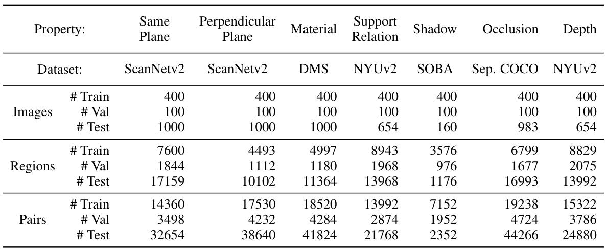
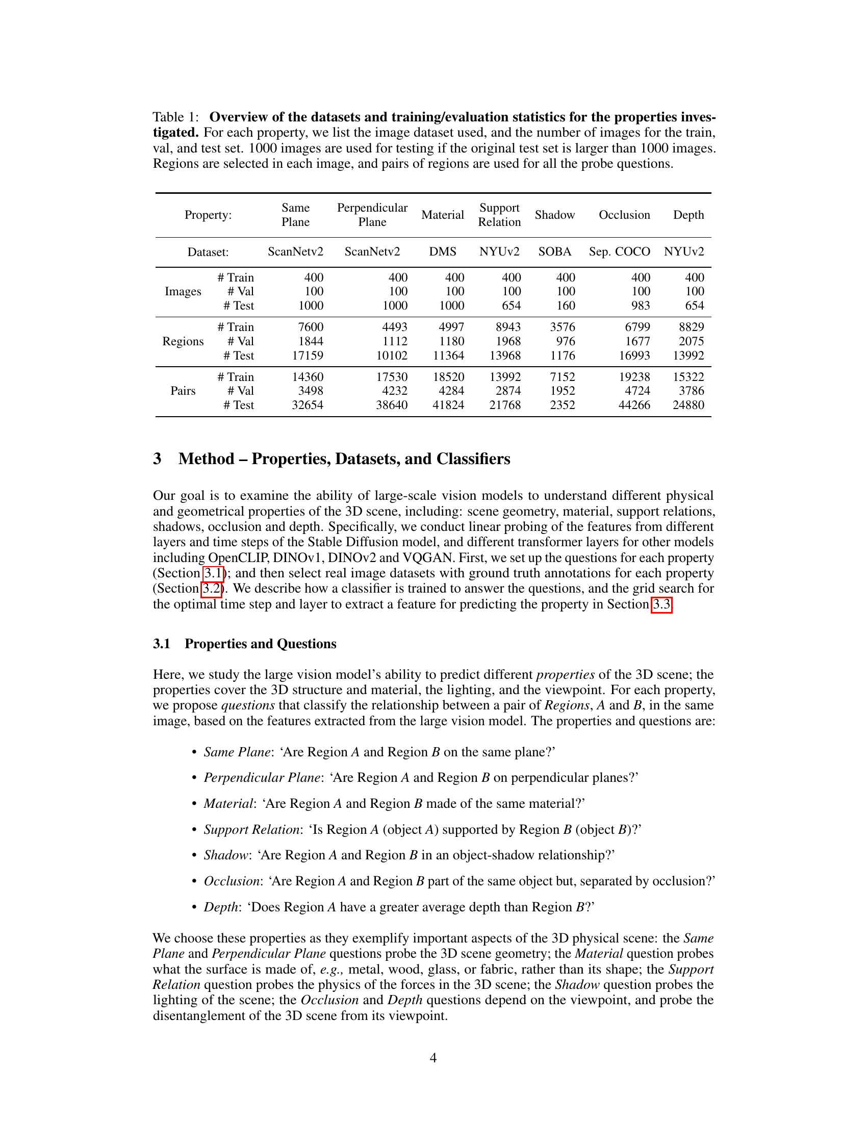
🔼 This table presents a summary of the datasets used for evaluating different 3D scene properties. For each property (Same Plane, Perpendicular Plane, Material, Support Relation, Shadow, Occlusion, Depth), it lists the dataset used, the number of images in the training, validation, and test sets, the number of regions selected in each image, and the number of region pairs used for training, validation, and testing. It shows the data split and size for training the linear classifiers used to evaluate the ability of different large vision models to predict the different properties.
read the caption
Table 1: Overview of the datasets and training/evaluation statistics for the properties investigated. For each property, we list the image dataset used, and the number of images for the train, val, and test set. 1000 images are used for testing if the original test set is larger than 1000 images. Regions are selected in each image, and pairs of regions are used for all the probe questions.
In-depth insights#
3D Prop. Probes#
The heading ‘3D Prop. Probes’ suggests an investigation into the capabilities of large vision models to understand three-dimensional physical properties. This likely involves probing the models with carefully designed datasets containing images annotated with various 3D properties, such as object geometry, material composition, lighting, shadows, occlusion and depth. The core idea is to assess how well the model’s internal representations capture these properties, potentially by training classifiers on extracted model features to predict these attributes. A key aspect would be evaluating the performance across different model architectures, investigating which models excel at representing specific properties and identifying the model layers or feature types most informative for these predictions. The success of this probing methodology hinges on the quality and diversity of the annotated datasets employed. Limitations of the approach would likely involve the difficulty in creating exhaustive and unbiased datasets covering all relevant properties and the challenge of interpreting classifier performance as a definitive measure of true 3D understanding.
Large Model Tests#
A hypothetical section titled “Large Model Tests” in a research paper would likely detail experiments evaluating the capabilities of large language models (LLMs). This would involve careful selection of benchmark datasets, representative of diverse tasks and complexities. The evaluation metrics would be crucial, going beyond simple accuracy to include measures of reasoning ability, bias, and robustness. Methodological details would be critical for reproducibility and transparency, covering data preprocessing, model training, and evaluation procedures. The analysis of results would extend beyond simple performance comparisons, examining the models’ strengths and weaknesses across various tasks. Qualitative analyses of model outputs could be insightful to explain patterns and potential limitations. Finally, the results would be discussed in the context of existing literature, highlighting novel contributions and implications for the field.
SD Feature Maps#
The heading ‘SD Feature Maps’ likely refers to feature maps extracted from a Stable Diffusion model. These maps represent the model’s internal representations of an image at different processing stages. Analyzing these maps offers insights into how Stable Diffusion understands and processes visual information, revealing which features are activated for specific image properties like geometry, materials, or lighting. Different layers within the model will likely reveal different levels of abstraction, with earlier layers capturing low-level details and later layers encoding higher-level semantic information. The use of SD Feature Maps in the study, likely involves probing the model’s 3D understanding, by training classifiers to predict various physical properties based on the feature maps. This approach could reveal whether the model encodes implicit 3D knowledge within its representations, and highlight which layers or stages are most crucial for 3D reasoning. Investigating these maps helps to unveil the ‘black box’ nature of large vision models, fostering a deeper comprehension of their internal mechanisms.
Downstream Tasks#
The concept of “Downstream Tasks” in the context of a research paper focusing on large vision models signifies the application of learned representations from pre-trained models to solve specific, practical problems. These tasks represent a significant departure from the initial training phase, which usually involves massive datasets and general objectives. Success in downstream tasks validates the generalizability and transfer learning capabilities of the pre-trained models. The choice of downstream tasks is crucial, as it reveals the strengths and weaknesses of the model’s learned representations. Tasks involving 3D scene understanding, such as depth estimation or surface normal prediction, would effectively assess the model’s ability to extract and utilize 3D information from 2D images. Conversely, simpler tasks might reveal that these large models have implicitly learned lower-level features. The performance on these varied downstream tasks would offer a holistic evaluation of the model, surpassing simple benchmark metrics. The results highlight areas ripe for improvement and inspire the design of more effective and robust pre-training strategies. Careful selection and execution of downstream tasks are, therefore, central to a comprehensive evaluation of large vision models and their potential for real-world applications.
Future Directions#
Future research could explore expanding the range of 3D physical properties investigated beyond the current set, incorporating more nuanced properties like contact relations and object orientation. Improving the robustness of the method to handle noisy or incomplete annotations is also crucial for wider applicability. Furthermore, investigating the effectiveness of the proposed protocol on diverse network architectures and training paradigms would enhance its generalizability. A promising area is to assess whether these probed properties can be leveraged effectively for downstream tasks such as scene completion, object pose estimation, or novel view synthesis. This could validate the practical utility of the findings. Finally, exploring advanced probing methods beyond linear classifiers, perhaps employing attention mechanisms or other explainability techniques, might unveil more nuanced insights into the 3D reasoning capabilities of large vision models.
More visual insights#
More on figures
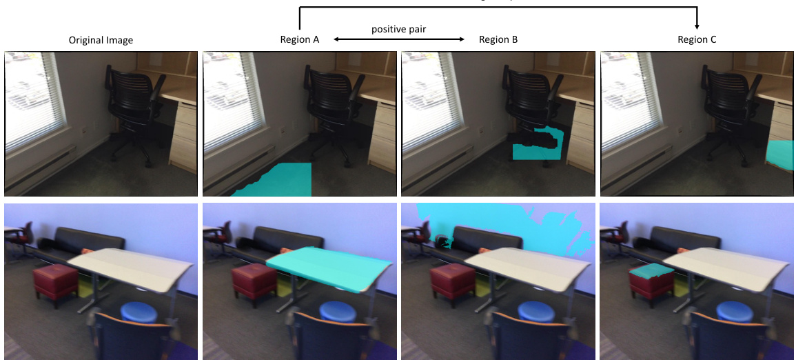
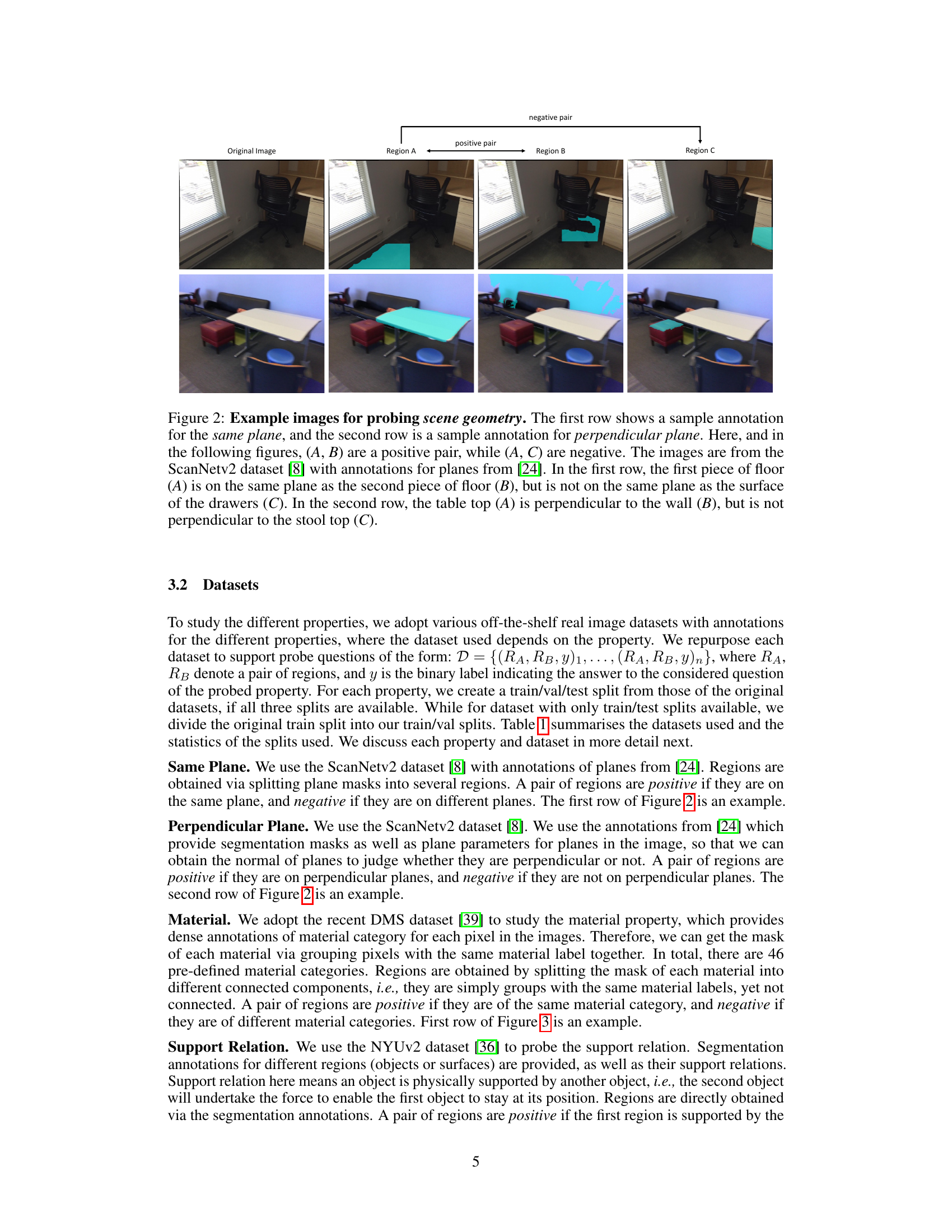
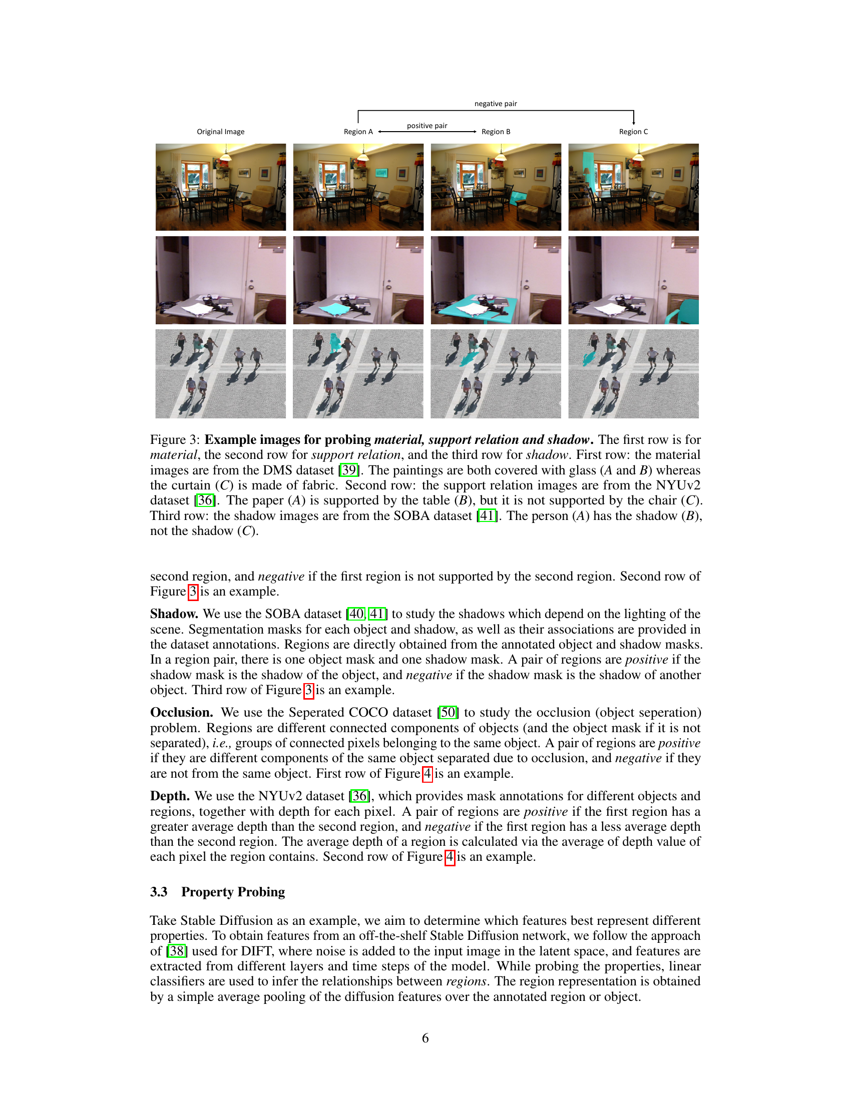
🔼 This figure shows example images used to test the model’s ability to understand scene geometry, specifically whether two regions are on the same plane or perpendicular planes. Each row presents an original image with annotated regions (A, B, C). Region pairs (A, B) represent positive examples of the geometric relationship (same plane or perpendicular), while (A, C) show negative examples.
read the caption
Figure 2: Example images for probing scene geometry. The first row shows a sample annotation for the same plane, and the second row is a sample annotation for perpendicular plane. Here, and in the following figures, (A, B) are a positive pair, while (A, C) are negative. The images are from the ScanNetv2 dataset [8] with annotations for planes from [24]. In the first row, the first piece of floor (A) is on the same plane as the second piece of floor (B), but is not on the same plane as the surface of the drawers (C). In the second row, the table top (A) is perpendicular to the wall (B), but is not perpendicular to the stool top (C).
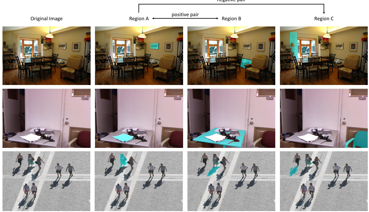
🔼 This figure shows example images used for evaluating three different properties: material, support relation, and shadow. Each row represents a different property with a positive and negative example pair. The image datasets used are DMS for material, NYUv2 for support relation and SOBA for shadow.
read the caption
Figure 3: Example images for probing material, support relation and shadow. The first row is for material, the second row for support relation, and the third row for shadow. First row: the material images are from the DMS dataset [39]. The paintings are both covered with glass (A and B) whereas the curtain (C) is made of fabric. Second row: the support relation images are from the NYUv2 dataset [36]. The paper (A) is supported by the table (B), but it is not supported by the chair (C). Third row: the shadow images are from the SOBA dataset [41]. The person (A) has the shadow (B), not the shadow (C).
🔼 This figure shows example images used to test the model’s ability to understand scene geometry, specifically whether two regions are on the same plane or perpendicular planes. Each row shows an example of a positive pair (A,B) and a negative pair (A,C), where the positive pair shares the property of interest (same plane or perpendicular plane) and the negative pair does not.
read the caption
Figure 2: Example images for probing scene geometry. The first row shows a sample annotation for the same plane, and the second row is a sample annotation for perpendicular plane. Here, and in the following figures, (A, B) are a positive pair, while (A, C) are negative. The images are from the ScanNetv2 dataset [8] with annotations for planes from [24]. In the first row, the first piece of floor (A) is on the same plane as the second piece of floor (B), but is not on the same plane as the surface of the drawers (C). In the second row, the table top (A) is perpendicular to the wall (B), but is not perpendicular to the stool top (C).

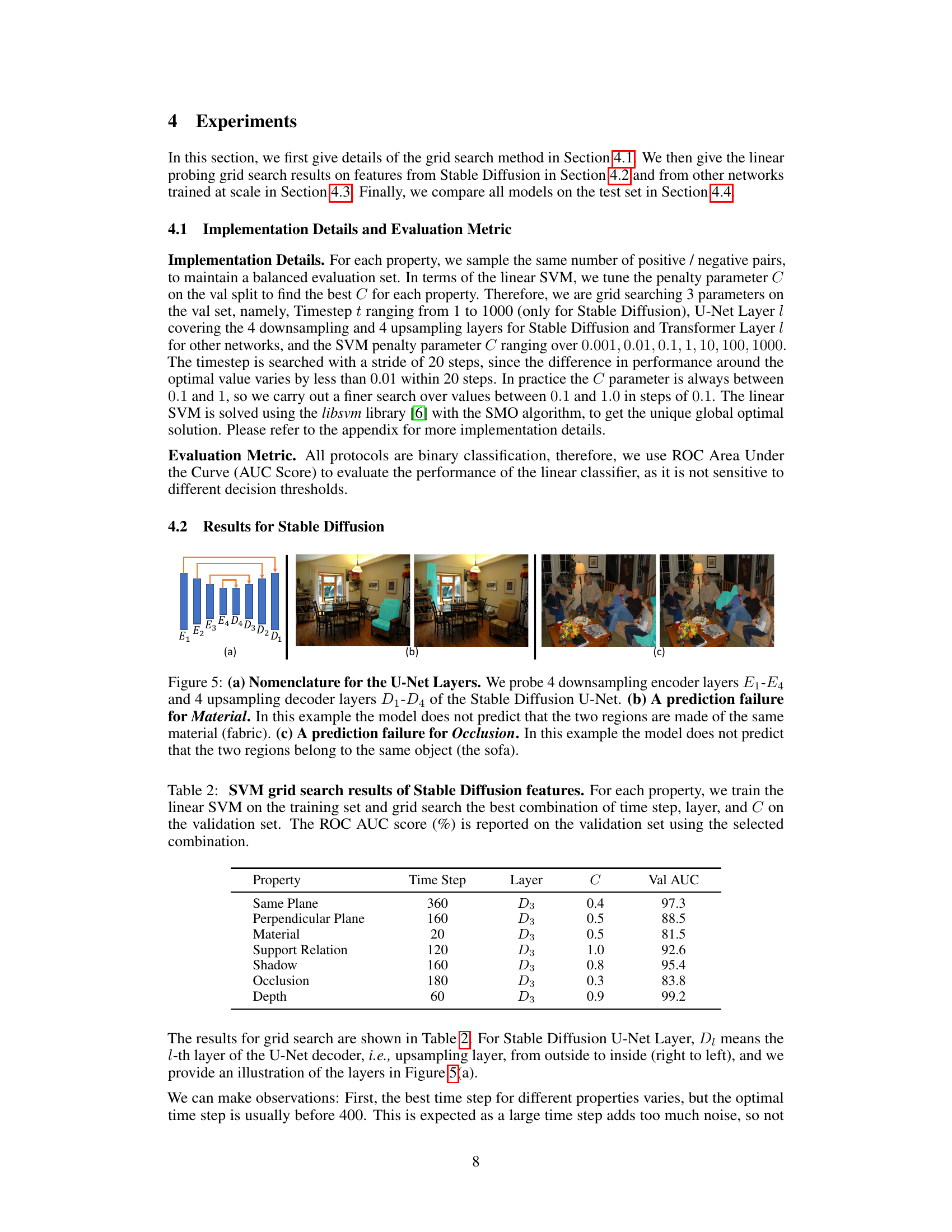
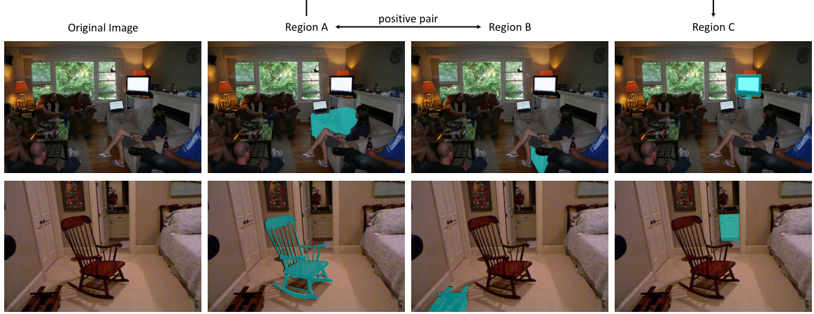
🔼 This figure shows the architecture of the U-Net used in Stable Diffusion and illustrates two prediction failures. (a) labels the encoder (E1-E4) and decoder (D1-D4) layers of the U-Net. (b) shows an example where the model incorrectly predicts the material of two regions. (c) shows an example where the model fails to identify that two regions belong to the same occluded object.
read the caption
Figure 5: (a) Nomenclature for the U-Net Layers. We probe 4 downsampling encoder layers E1-E4 and 4 upsampling decoder layers D1-D4 of the Stable Diffusion U-Net. (b) A prediction failure for Material. In this example the model does not predict that the two regions are made of the same material (fabric). (c) A prediction failure for Occlusion. In this example the model does not predict that the two regions belong to the same object (the sofa).
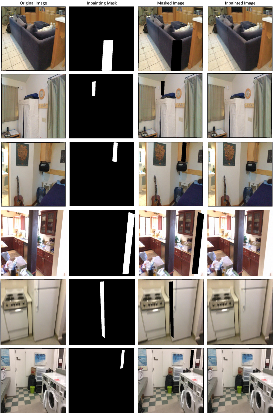
🔼 This figure showcases Stable Diffusion’s ability to predict scene geometry, specifically focusing on same-plane and perpendicular-plane relationships. The model successfully inpaints masked regions in real images, demonstrating an understanding of how planes intersect to form corners, even when only part of the planes are visible.
read the caption
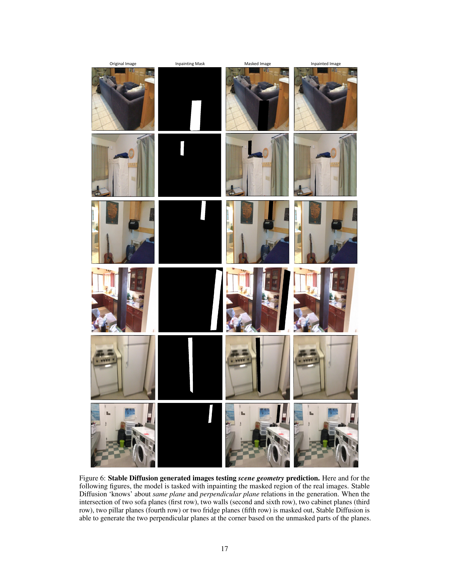
Figure 6: Stable Diffusion generated images testing scene geometry prediction. Here and for the following figures, the model is tasked with inpainting the masked region of the real images. Stable Diffusion 'knows' about same plane and perpendicular plane relations in the generation. When the intersection of two sofa planes (first row), two walls (second and sixth row), two cabinet planes (third row), two pillar planes (fourth row) or two fridge planes (fifth row) is masked out, Stable Diffusion is able to generate the two perpendicular planes at the corner based on the unmasked parts of the planes.
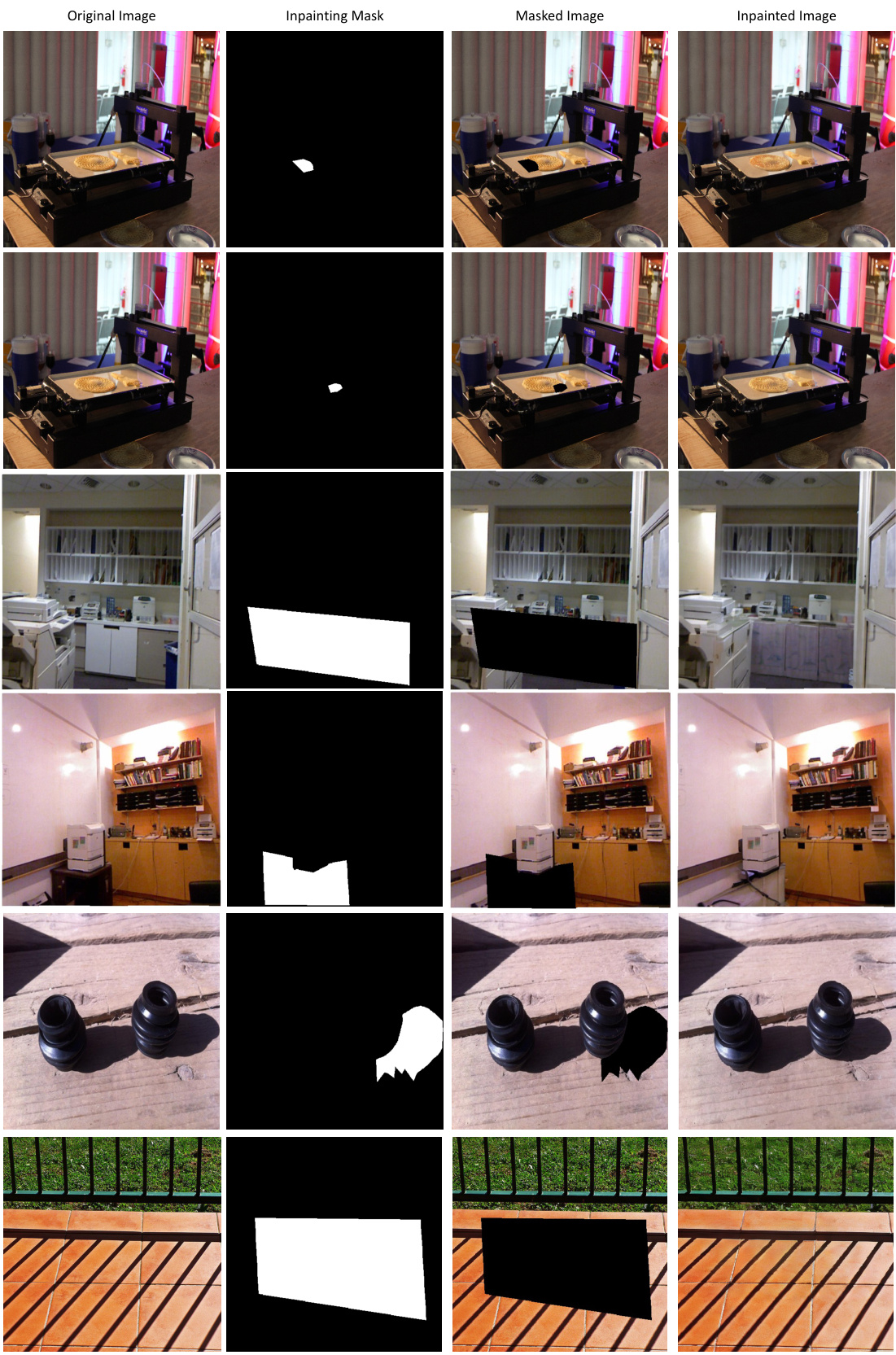
🔼 This figure shows examples of Stable Diffusion inpainting images for material, support relation, and shadow. The model performs well on support relation and shadow prediction, but struggles with material prediction when the boundary between materials is unclear.
read the caption
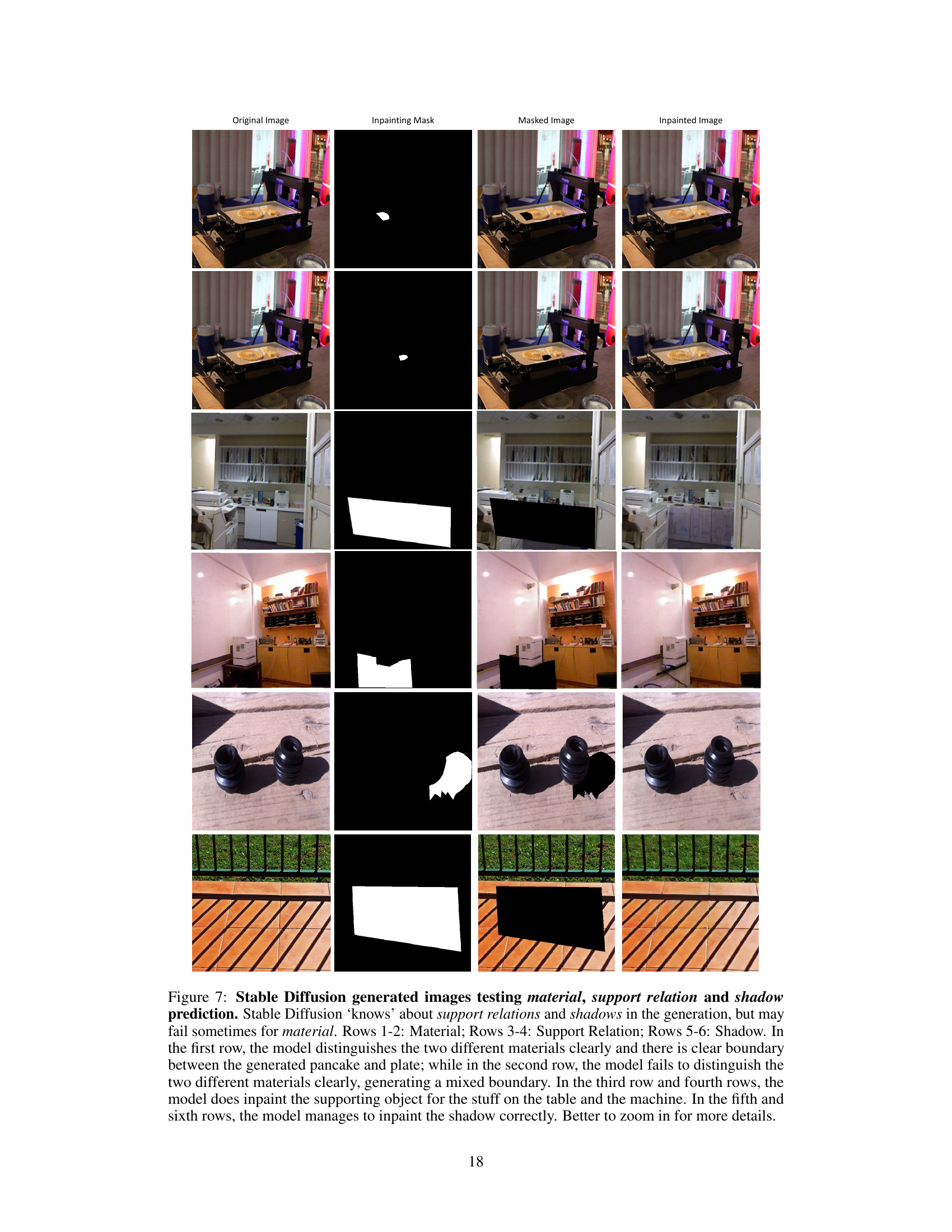
Figure 7: Stable Diffusion generated images testing material, support relation and shadow prediction. Stable Diffusion ‘knows’ about support relations and shadows in the generation, but may fail sometimes for material. Rows 1–2: Material; Rows 3–4: Support Relation; Rows 5–6: Shadow. In the first row, the model distinguishes the two different materials clearly and there is clear boundary between the generated pancake and plate; while in the second row, the model fails to distinguish the two different materials clearly, generating a mixed boundary. In the third row and fourth rows, the model does inpaint the supporting object for the stuff on the table and the machine. In the fifth and sixth rows, the model manages to inpaint the shadow correctly. Better to zoom in for more details.
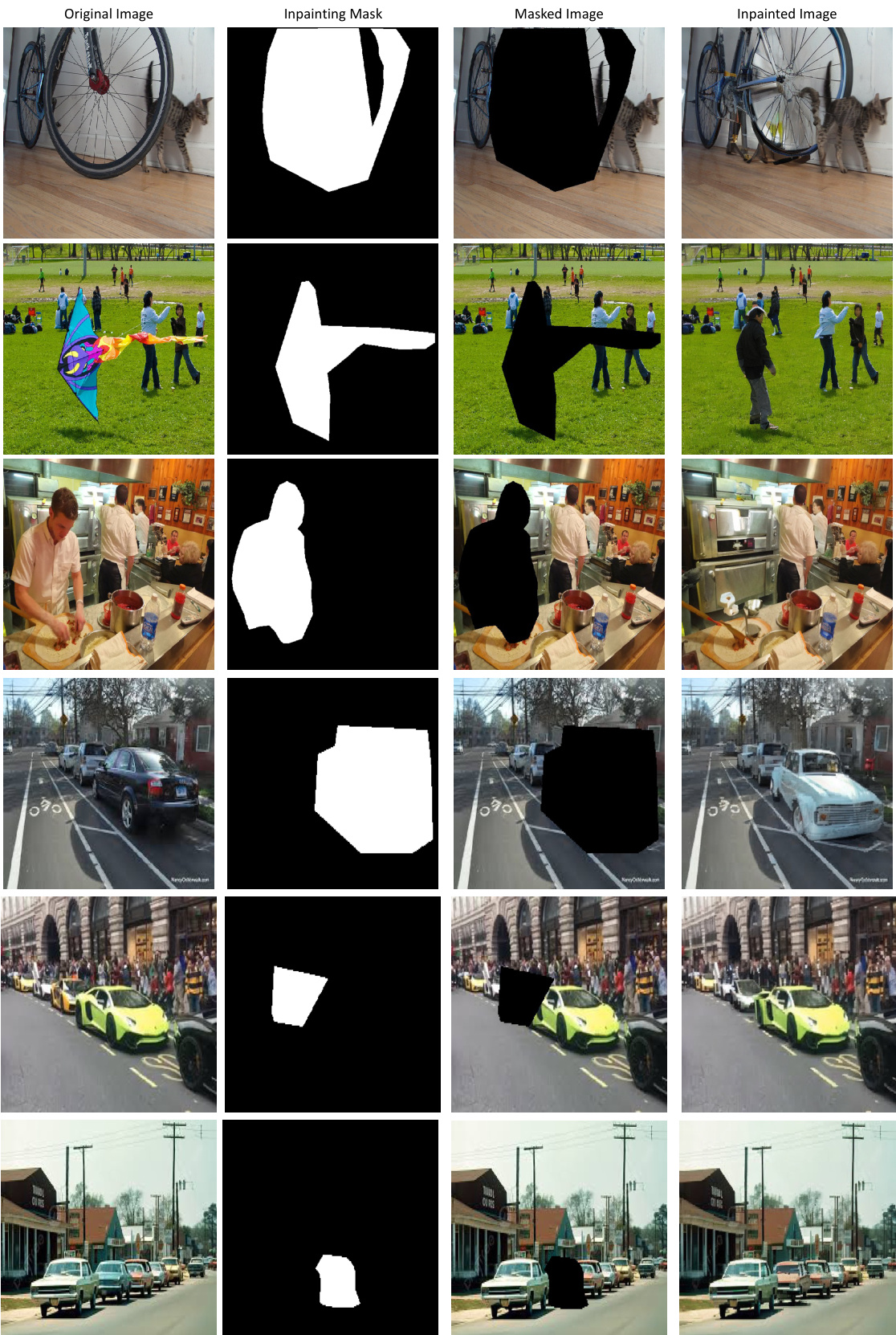
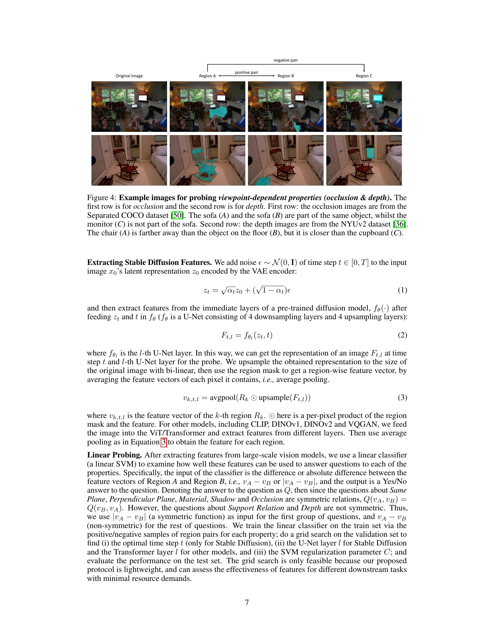
🔼 This figure shows examples of Stable Diffusion’s image inpainting results, demonstrating its ability to predict depth accurately but sometimes failing to correctly handle occlusions. The figure includes six examples, with the first three focusing on occlusions and the latter three on depth perception.
read the caption
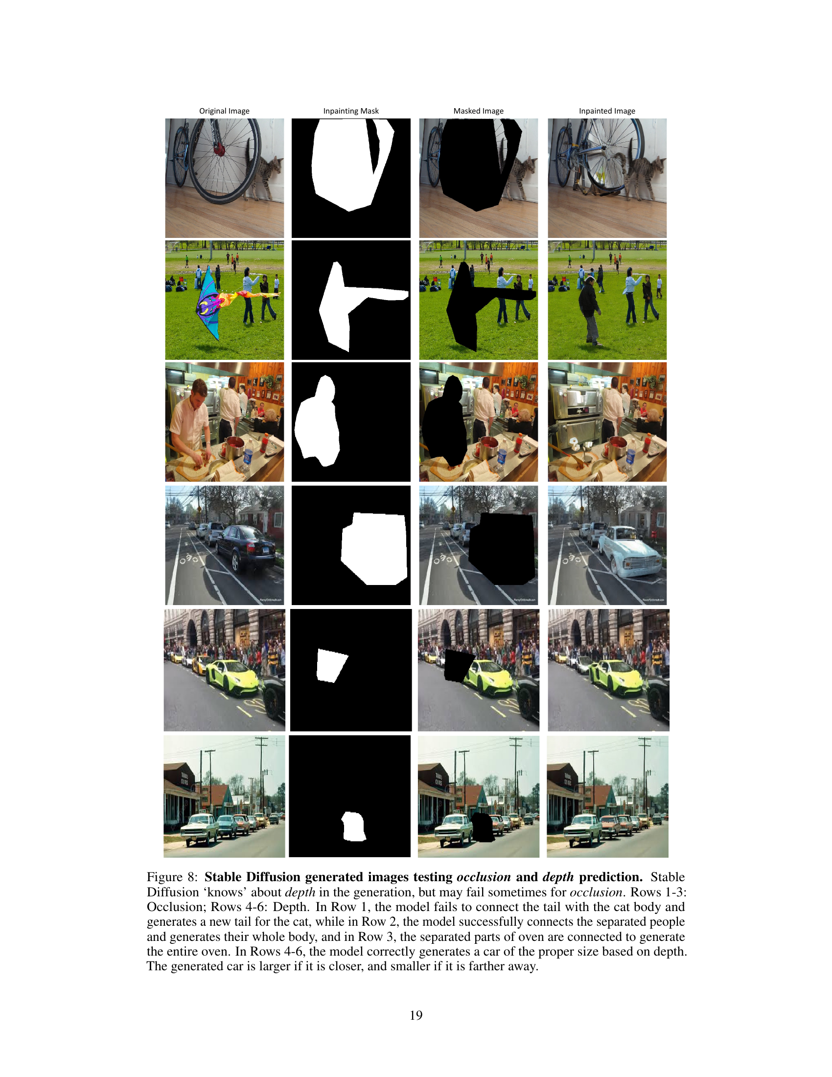
Figure 8: Stable Diffusion generated images testing occlusion and depth prediction. Stable Diffusion ‘knows’ about depth in the generation, but may fail sometimes for occlusion. Rows 1–3: Occlusion; Rows 4–6: Depth. In Row 1, the model fails to connect the tail with the cat body and generates a new tail for the cat, while in Row 2, the model successfully connects the separated people and generates their whole body, and in Row 3, the separated parts of oven are connected to generate the entire oven. In Rows 4–6, the model correctly generates a car of the proper size based on depth. The generated car is larger if it is closer, and smaller if it is farther away.
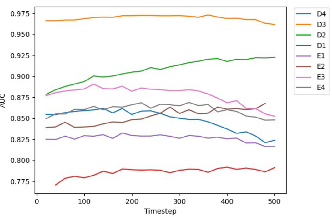
🔼 This figure shows the Area Under the Curve (AUC) values for different layers (D1-D4, E1-E4) and timesteps of the Stable Diffusion model when performing the ‘same plane’ task. The x-axis represents the timestep, and the y-axis represents the AUC score. Each line corresponds to a different layer within the Stable Diffusion model. The plot illustrates how the performance (AUC) of the model changes for the same-plane prediction task across different layers and different timesteps of the diffusion process.
read the caption
Figure 9: Curves for AUC at different layers and time steps of probing Stable Diffusion for the same plane task.
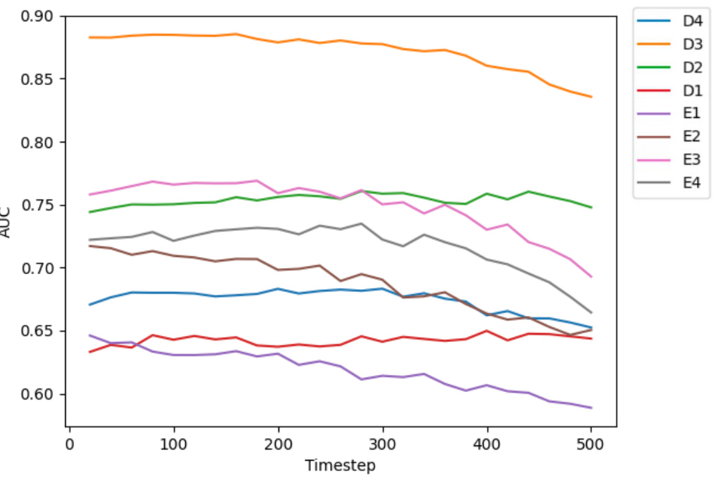
🔼 This figure shows the Area Under the Curve (AUC) values obtained for the ‘perpendicular plane’ task using Stable Diffusion. Different curves represent different layers (D1-D4, E1-E4) of the U-Net within the Stable Diffusion model. The x-axis represents the different time steps used during the diffusion process, illustrating how the AUC varies across layers and time steps. The overall trend helps to determine the optimal layers and time steps for maximizing performance on this specific task of identifying perpendicular planes.
read the caption
Figure 10: Curves for AUC at different layers and time steps of probing Stable Diffusion for the perpendicular plane task.
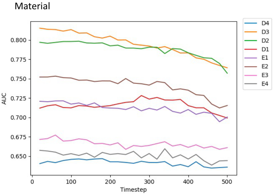
🔼 This figure shows the Area Under the Curve (AUC) values for different layers (D1-D4, E1-E4) and timesteps of the Stable Diffusion model when applied to the material property prediction task. Each line represents a specific layer, and the x-axis represents different timesteps in the diffusion process. The y-axis shows the AUC, measuring the model’s performance in distinguishing between different materials. The graph helps analyze which layers and timesteps of the Stable Diffusion model are most effective for material property prediction.
read the caption
Figure 11: Curves for AUC at different layers and time steps of probing Stable Diffusion for the material task.
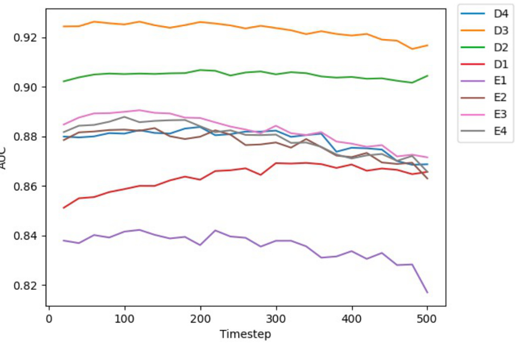
🔼 This figure shows the Area Under the Curve (AUC) for different layers (D1-D4, E1-E4) and timesteps of the Stable Diffusion model when performing the ‘same plane’ task. The x-axis represents the timestep, ranging from 0 to 500, and the y-axis represents the AUC score, indicating the model’s performance at classifying whether two regions are on the same plane. Each line corresponds to a different layer of the model, showing how the model’s performance varies across different layers and timesteps.
read the caption
Figure 9: Curves for AUC at different layers and time steps of probing Stable Diffusion for the same plane task.
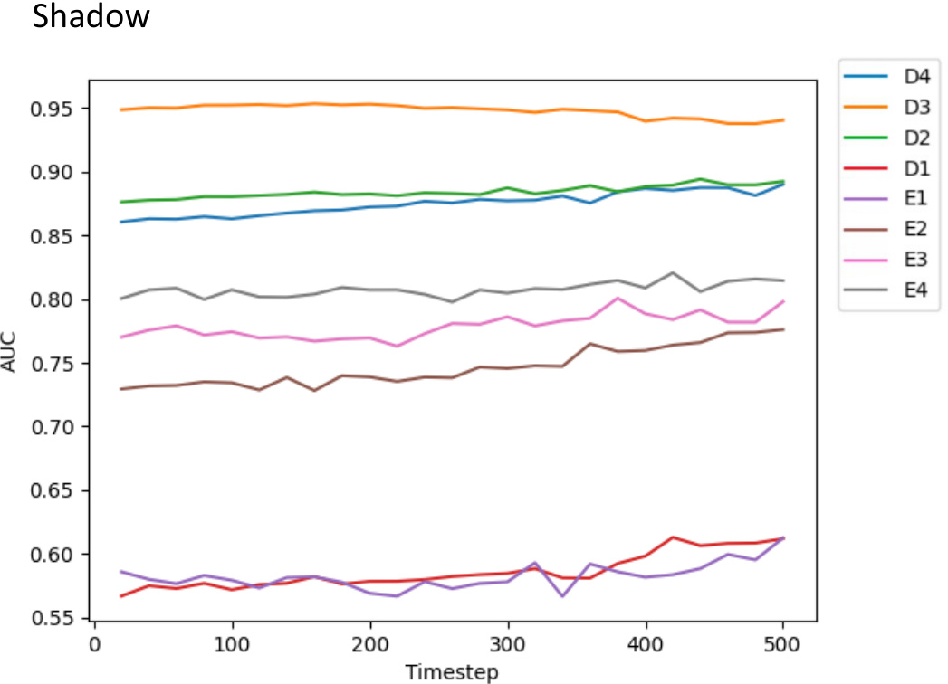
🔼 This figure shows the Area Under the Curve (AUC) values obtained for different layers and timesteps when probing the Stable Diffusion model’s ability to predict shadows. The x-axis represents the timestep, and the y-axis represents the AUC score. Different lines represent different layers in the model (D1-D4, E1-E4). The graph helps to understand which layer and timestep combination performs best for shadow prediction in the Stable Diffusion model.
read the caption
Figure 13: Curves for AUC at different layers and time steps of probing Stable Diffusion for the shadow task.
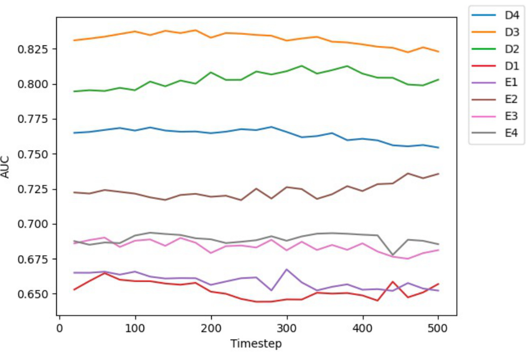
🔼 This figure shows the Area Under the Curve (AUC) values obtained when probing different layers and timesteps of the Stable Diffusion model for the ‘same plane’ task. The x-axis represents the timestep in the diffusion process, and the y-axis shows the AUC score which indicates how well the model can distinguish between pairs of regions that are on the same plane versus those that are not. Each line represents a different layer within the U-Net architecture of Stable Diffusion (D1-D4 representing decoder layers and E1-E4 representing encoder layers). The curves illustrate the performance of different layers at different timesteps, allowing researchers to identify which layer and timestep combination is most effective for this specific task in 3D scene understanding.
read the caption
Figure 9: Curves for AUC at different layers and time steps of probing Stable Diffusion for the same plane task.
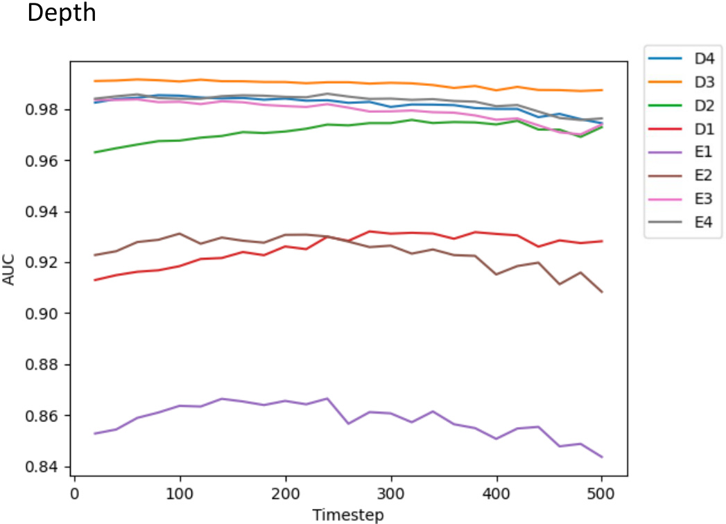
🔼 This figure shows the Area Under the Curve (AUC) values obtained from using features extracted from different layers (D1-D4, E1-E4) and timesteps (0-500) of the Stable Diffusion model for a depth prediction task. The plot helps to visualize how the performance of the model varies across different layers and timesteps. It indicates the optimal layers and timesteps to extract features for the depth prediction task.
read the caption
Figure 15: Curves for AUC at different layers and time steps of probing Stable Diffusion for the depth task.
More on tables

🔼 This table presents the hyperparameters and performance of a linear Support Vector Machine (SVM) trained on Stable Diffusion features for seven different 3D scene properties. For each property, the optimal time step, layer, and regularization parameter (C) were determined through grid search on a validation set. The table shows the resulting validation AUC (Area Under the ROC Curve) scores, indicating the model’s performance in classifying the property.
read the caption
Table 2: SVM grid search results of Stable Diffusion features. For each property, we train the linear SVM on the training set and grid search the best combination of time step, layer, and C on the validation set. The ROC AUC score (%) is reported on the validation set using the selected combination.

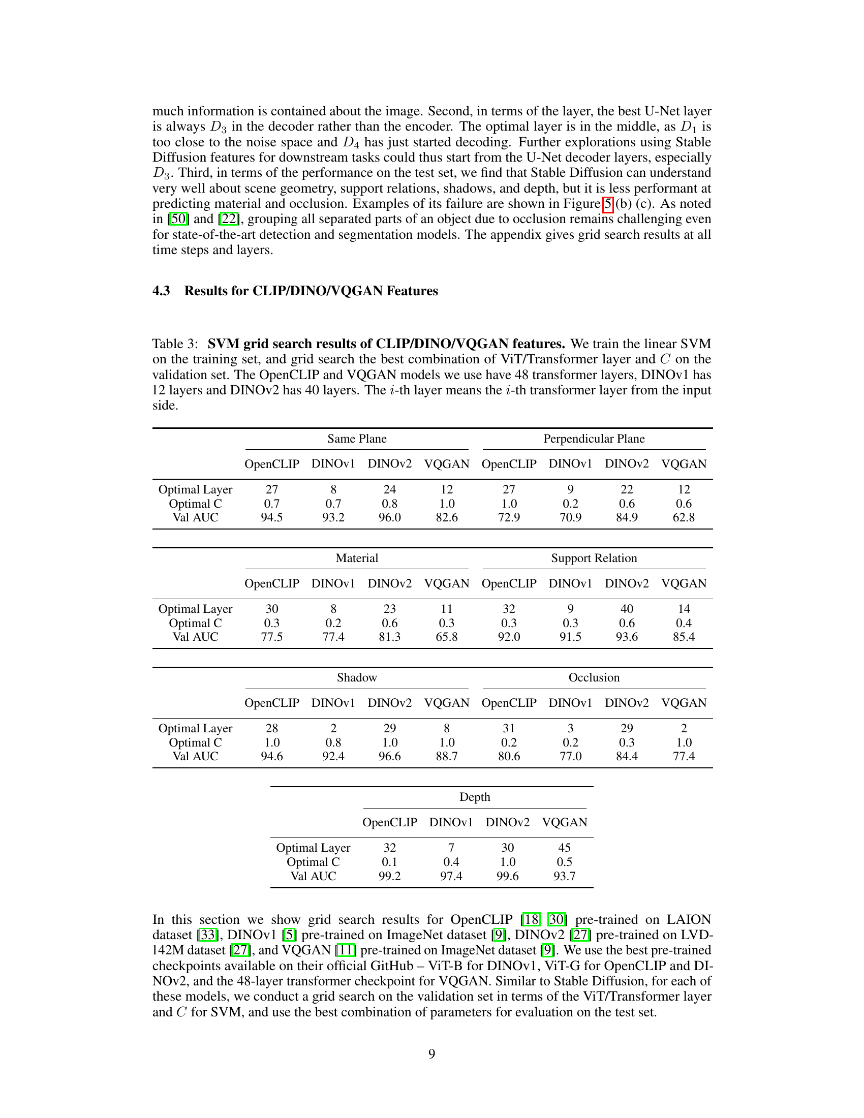
🔼 This table presents the results of a grid search performed to find the optimal hyperparameters for different pre-trained vision models (CLIP, DINOv1, DINOv2, VQGAN) when used for a linear probing task. The grid search involved selecting the best transformer layer and regularization parameter (C) for an SVM classifier to predict different 3D scene properties. The table shows the optimal layer and C value found, along with the resulting validation AUC score for each property and model.
read the caption
Table 3: SVM grid search results of CLIP/DINO/VQGAN features. We train the linear SVM on the training set, and grid search the best combination of ViT/Transformer layer and C on the validation set. The OpenCLIP and VQGAN models we use have 48 transformer layers, DINOv1 has 12 layers and DINOv2 has 40 layers. The i-th layer means the i-th transformer layer from the input side.

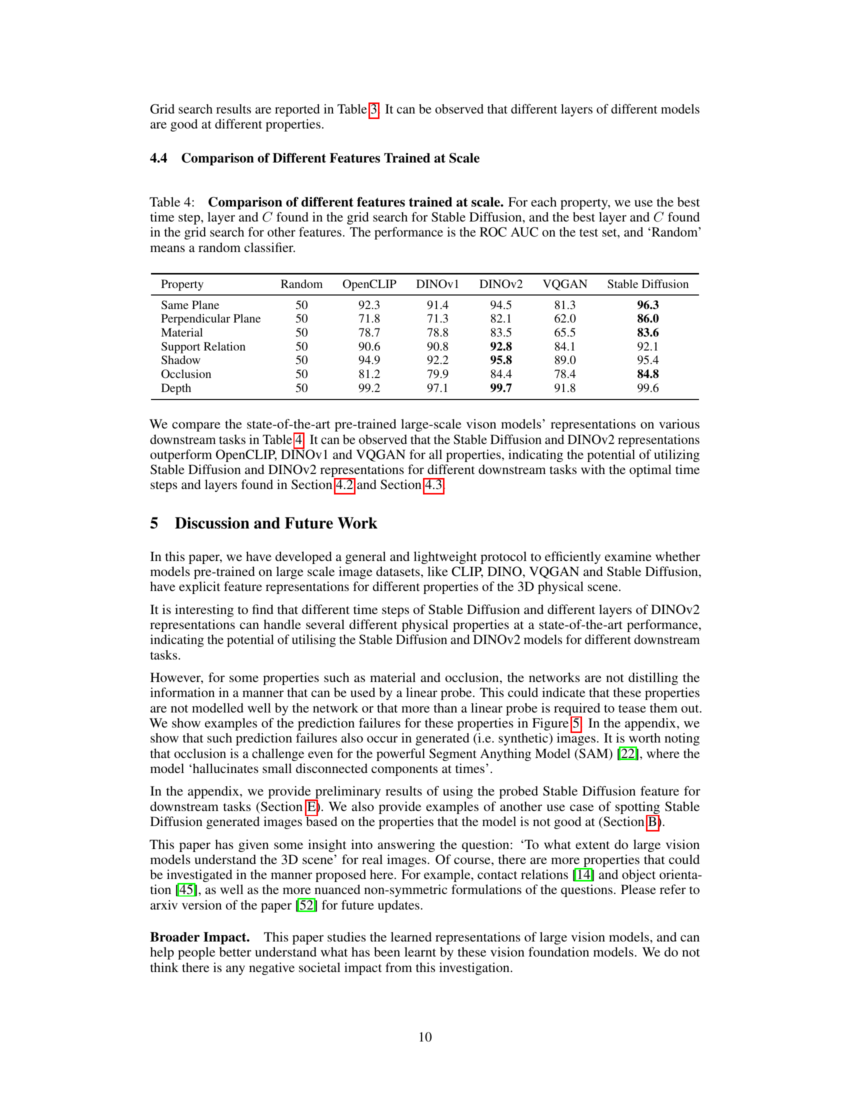
🔼 This table compares the performance of different large-scale vision models (OpenCLIP, DINOv1, DINOv2, VQGAN, and Stable Diffusion) on various downstream tasks related to 3D physical scene understanding. For each property (Same Plane, Perpendicular Plane, etc.), the best hyperparameters from a grid search are used for each model. The results are presented as the area under the ROC curve (AUC) on a test set, comparing each model against a random classifier.
read the caption
Table 4: Comparison of different features trained at scale. For each property, we use the best time step, layer and C found in the grid search for Stable Diffusion, and the best layer and C found in the grid search for other features. The performance is the ROC AUC on the test set, and 'Random' means a random classifier.
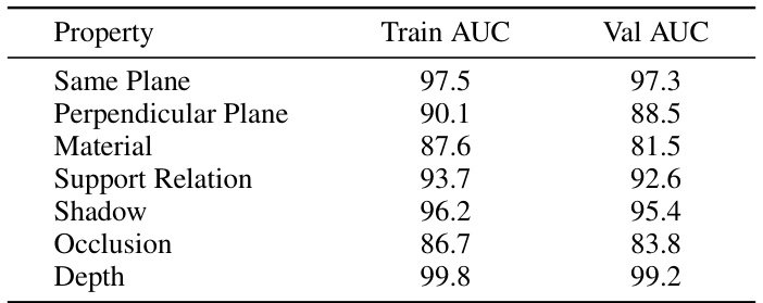
🔼 This table presents the training and validation AUC scores achieved by a Support Vector Machine (SVM) using features extracted from the Stable Diffusion model. The best performing time step, layer, and regularization parameter (C) were determined through grid search for each of the seven properties investigated (Same Plane, Perpendicular Plane, Material, Support Relation, Shadow, Occlusion, and Depth). The AUC scores indicate the model’s ability to discriminate between positive and negative examples for each property using the Stable Diffusion features.
read the caption
Table 5: Train/Val AUC of SVM grid search for Stable Diffusion features. For each property, the Train/Val AUC at the best combination of time step, layer and C is reported.

🔼 This table shows the results of using features from Stable Diffusion, selected by the authors’ probing method, for the task of surface normal estimation. The features were injected into the iDisc model [29], and the results are compared to the original iDisc model’s performance. The metrics used for comparison include Mean Angular Error, Angular RMSE, and percentages of angles less than 11.25, 22.5, and 30 degrees.
read the caption
Table 6: Preliminary results of using the probed feature for the downstream task of normal estimation. Here we show the results of injecting the selected Stable Diffusion feature into iDisc [29]. Please see text for more details.

🔼 This table shows the comparison of depth estimation performance using features from ResNet-50 and Stable Diffusion (SD). The performance is measured by three metrics (δ₁, δ₂, δ₃) representing the percentage of pixels with relative depth errors less than 11.25%, 22.5%, and 30%, respectively, and RMSE (Root Mean Squared Error) representing the overall accuracy. SD features significantly outperform ResNet-50 features across all metrics, indicating the potential of using probed SD features for depth estimation.
read the caption
Table 7: Preliminary results of using the probed feature for downstream task of depth estimation. Here we show the results of a comparison between ResNet and SD features on the NYUv2 Depth test dataset. Please see text for more details.
Full paper#
