TL;DR#
Offline reinforcement learning often struggles with long-term planning, especially when step-wise rewards are unavailable or sparse. Existing methods like Decision Transformer (DT) rely on return-to-go (RTG) estimations, which can be unreliable in such scenarios. This leads to inconsistencies in credit assignment and difficulties in learning temporally consistent policies. Furthermore, DT can struggle with trajectory stitching, combining suboptimal trajectories to achieve better overall results.
The proposed Latent Plan Transformer (LPT) tackles these issues by using a latent variable to represent a ‘plan’, connecting trajectory generation and the final return. Instead of relying on RTGs, LPT learns the joint distribution of trajectories and returns, allowing it to infer the plan from the expected return before policy execution. The method utilizes a Transformer-based architecture and posterior sampling, demonstrating the effectiveness of planning through latent space inference. LPT shows strong empirical results across diverse benchmarks, outperforming existing methods in tasks with sparse and delayed rewards, showcasing its capability in credit assignment, and trajectory stitching.
Key Takeaways#
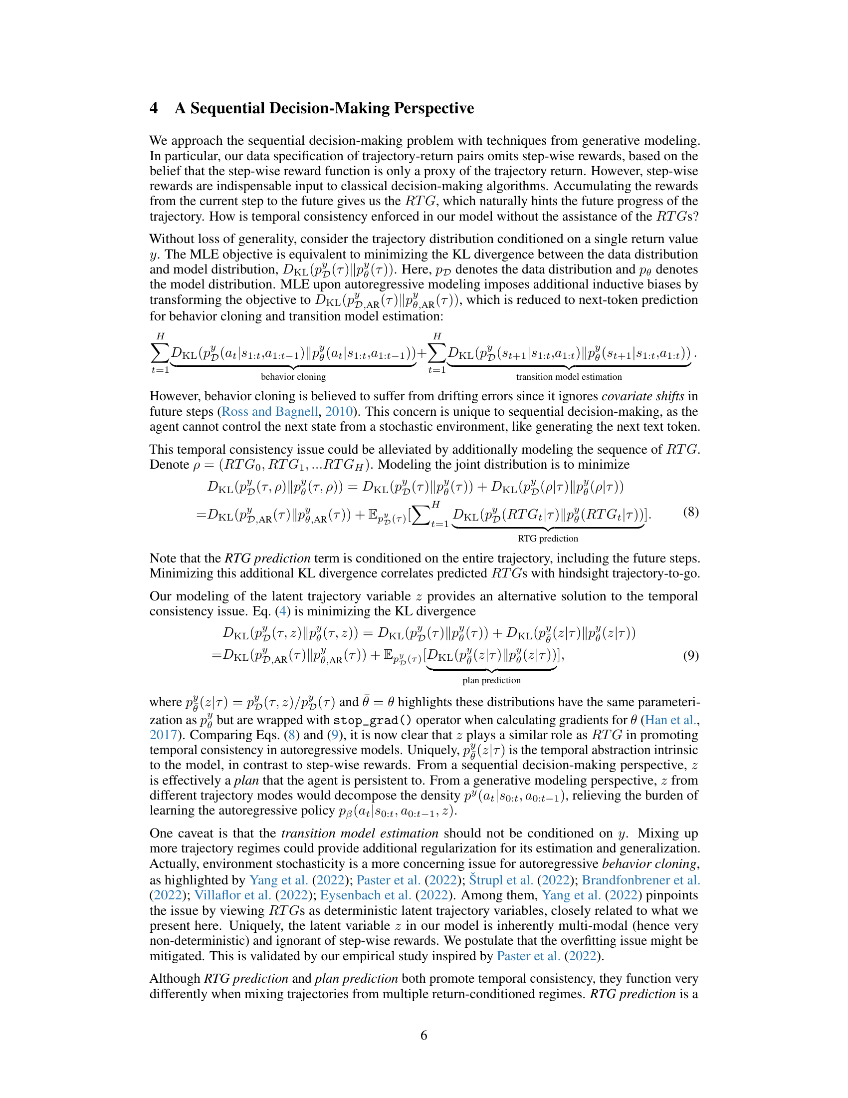
Why does it matter?#
This paper is important because it presents a novel approach to long-term planning in reinforcement learning, addressing the challenge of temporal consistency without relying on step-wise rewards. It offers a strong alternative to traditional reward-prompting methods, opening up new avenues for research in offline RL and generative models for decision-making. Its empirical success across diverse benchmarks validates the potential of latent variable inference for planning and its effectiveness in handling sparse and delayed rewards.
Visual Insights#
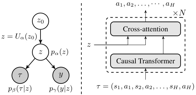
🔼 The figure illustrates the Latent Plan Transformer (LPT) model. The left panel shows the overall architecture, highlighting the latent variable z connecting the trajectory generator and return predictor. The latent variable is generated from a prior distribution (z = Ua(zo)). Given z, the trajectory and return are conditionally independent. The right panel focuses on the trajectory generator, illustrating how it uses a causal transformer and cross-attention with z to generate the trajectory sequence.
read the caption
Figure 1: Left: Overview of Latent Plan Transformer (LPT). z ∈ Rd is the latent vector. The prior distribution of z is a neural transformation of zo, i.e., z = Ua(zo), zo ~ N(0, Ia). Given z, τ and y are independent. ps(T|z) is the trajectory generator. py(y|z) is the return predictor. Right: Illustration of trajectory generator ps(T|z).

🔼 This table presents the performance comparison of the proposed Latent Plan Transformer (LPT) model against several baseline methods (CQL, DT, QDT) on various OpenAI Gym MuJoCo tasks. The results are categorized by two data specifications: one with step-wise rewards and another with only the final return. The table shows the final return achieved by each method across different tasks, highlighting the superior performance of LPT, especially when only the final return is provided as input.
read the caption
Table 1: Evaluation results of offline OpenAI Gym MuJoCo tasks. We provide results for data specification with step-wise reward (left) and final return (right). Bold highlighting indicates top scores. LPT outperforms all final-return baselines and most step-wise-reward baselines.
In-depth insights#
Latent Plan Inference#
The concept of ‘Latent Plan Inference’ suggests a powerful approach to AI planning. Instead of relying on explicit, step-wise rewards, it infers a high-level plan from a desired outcome (e.g., a high reward). This plan, represented as a latent variable, guides the system’s actions, effectively decoupling trajectory generation from immediate reward signals. This framework offers several advantages: it reduces reliance on meticulously designed reward functions, enabling adaptation to complex and uncertain environments; it allows for more nuanced credit assignment by connecting actions to the ultimate goal; and it facilitates trajectory stitching, combining suboptimal trajectories to achieve the desired outcome. The inference process itself becomes a form of planning, providing a strong alternative to step-wise reward prompting and potentially enhancing long-range planning capabilities. However, challenges remain, particularly in dealing with highly stochastic environments and ensuring the inferred plans are robust and generalize well. Further research into the properties of the latent space and the effectiveness of the inference method is crucial to fully realize the potential of this approach.
Offline RL Approach#
Offline reinforcement learning (RL) tackles the challenge of learning policies from pre-collected datasets, without the need for online interaction with the environment. This approach is particularly valuable in scenarios where online data collection is expensive, dangerous, or impossible. A key advantage is the ability to leverage large, previously gathered datasets which can significantly speed up the learning process and improve the performance of the resulting policy. However, offline RL presents significant challenges. The primary difficulty stems from the distribution mismatch between the training data and the states encountered during deployment. The learned policy may perform poorly in states not well-represented in the training data. Addressing this requires careful consideration of data quality, algorithm design, and evaluation metrics. Techniques such as importance weighting, behavior cloning, and conservative Q-learning aim to mitigate this distribution shift, but each has limitations. Effective offline RL strategies often incorporate sophisticated data augmentation, regularization, and constraints to improve robustness and generalization. The field is rapidly evolving, with ongoing research exploring new algorithms, data representations, and evaluation benchmarks to overcome the challenges and unlock the full potential of learning from offline data.
MCMC Posterior#
In the context of a research paper, a section on “MCMC Posterior” would delve into the application of Markov Chain Monte Carlo (MCMC) methods for estimating posterior distributions. This is crucial when dealing with complex probability models where direct calculation is intractable. The discussion would likely detail the specific MCMC algorithm used (e.g., Metropolis-Hastings, Gibbs sampling, Hamiltonian Monte Carlo), justifying its selection based on the problem’s characteristics. Key aspects would include the proposal distribution (how new samples are generated), acceptance criteria (determining whether a proposed sample is accepted or rejected), and convergence diagnostics (assessing whether the algorithm has adequately explored the posterior). A critical evaluation would address the algorithm’s efficiency, the impact of tuning parameters on performance, and potential limitations, such as slow convergence or sensitivity to initialization. The results section would showcase the posterior estimates obtained, perhaps visualized through density plots or other means. Finally, the implications of the obtained posterior would be discussed in relation to the research question, highlighting any insights gained or conclusions drawn.
Trajectory Stitching#
Trajectory stitching, a crucial challenge in offline reinforcement learning, focuses on the ability of an agent to combine suboptimal trajectory segments from a dataset to achieve a complete and optimal trajectory. This is especially relevant when dealing with sparse rewards or datasets lacking complete successful trajectories. The success of trajectory stitching hinges on the agent’s capability to identify and integrate relevant sub-trajectories, effectively learning temporal dependencies across disparate parts of the data. Latent variable models, like those presented in this paper, offer an elegant solution by providing an abstraction that integrates information from both the final return and sub-trajectories, enabling effective stitching. This contrasts with methods relying solely on step-wise rewards, which can struggle to handle temporally extended decision-making and sparse rewards inherent in many real-world scenarios. The effectiveness of trajectory stitching is crucial for achieving competitive performance, particularly in tasks requiring complex sequential actions and long-range planning, as demonstrated by the presented experimental results.
Future Work#
The “Future Work” section of this research paper presents exciting avenues for extending the Latent Plan Transformer (LPT). Expanding LPT’s capabilities to online settings and multi-agent scenarios is crucial. Online adaptation would enhance real-world applicability, while a multi-agent extension could unlock collaborations and complex interactions. Investigating the model’s potential in embodied agents is also highly promising. This exploration would extend LPT beyond simulations to physical robots, revealing its effectiveness in handling complex sensorimotor dynamics. Furthermore, a deeper theoretical analysis of LPT’s generalization capabilities is essential, providing a stronger foundation for its broader adoption. Finally, exploring LPT’s role in various real-world applications such as molecule design, where it has shown early success, warrants dedicated investigation. Addressing these areas will solidify LPT’s position as a leading generative model for planning.
More visual insights#
More on figures

🔼 This figure shows the comparison of trajectories generated by LPT and those from the training set in two different maze environments, Maze2D-medium and Maze2D-large. The left panels display example trajectories from the original training data, illustrating their suboptimal nature and frequent failures to reach the goal. In contrast, the right panels showcase trajectories generated by the Latent Plan Transformer (LPT) model, demonstrating its ability to generate more efficient and successful paths to the goal state. The yellow stars in each maze mark the location of the goal.
read the caption
Figure 2: (a) Maze2D-medium environment (b) Maze2D-large environment. Left panels show example trajectories from the training set and right panels show LPT generations. Yellow stars represent the goal states.
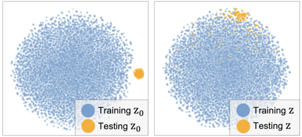
🔼 This figure visualizes the latent variable z in the Maze2D-medium environment. The left panel shows the training z0 samples from the aggregated posterior, while the right panel shows the distribution of z, which is transformed from z0. The colors differentiate between training and testing data. It illustrates the model’s ability to generate new trajectories that are similar to those in the training data, yet also capable of exploring unseen regions of the latent space, indicating the model’s generalization capability.
read the caption
Figure 3: t-SNE plot of latent variables in the Maze2D-medium. Left: Training z0 from aggregated posterior Ep(T,y)[pθ(z0|T,Y)]. Testing z0 from pθ(z0|y), disjoint from training population. Right: Distribution of z = Ua(z0).
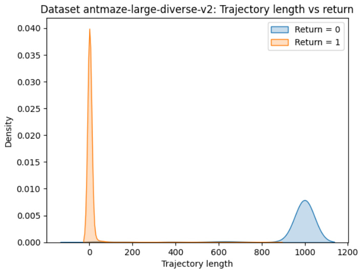
🔼 This figure shows the distribution of trajectory lengths and returns in the Antmaze-large-diverse dataset. The x-axis represents the length of the trajectory, and the y-axis represents the density. Two distributions are shown, one for trajectories with a return of 0 and another for trajectories with a return of 1. The distribution for trajectories with a return of 0 is heavily concentrated near a length of 1, while the distribution for trajectories with a return of 1 is concentrated around a length of 1000. This indicates a strong correlation between trajectory length and return in this dataset, with longer trajectories more likely to result in a successful return.
read the caption
Figure 4: Trajectory length and return distribution in dataset Antmaze-large-diverse

🔼 This figure shows the distribution of trajectory lengths and returns for the Maze2D-Large dataset. The top panel is a histogram of the returns, showing that most trajectories have a relatively low return, but there are some trajectories with much higher returns. The bottom panel is a histogram of the trajectory lengths, showing that the trajectory lengths are approximately normally distributed, with a mean around 250 steps. The combination of the two panels shows the relationship between trajectory length and return, with longer trajectories often yielding higher returns.
read the caption
Figure 5: Trajectory length and return distribution in dataset Maze2D-Large
More on tables

🔼 This table presents the performance comparison of different reinforcement learning algorithms (CQL, DT, QDT, LPT, and LPT-EI) on three different Maze2D tasks with varying complexities (umaze, medium, and large). The results are expressed as mean ± standard deviation and show the average scores achieved by each algorithm on the tasks. Bold highlights indicate the best-performing algorithm for each task. The table demonstrates LPT’s success in achieving superior performance compared to the other algorithms, particularly when combined with Exploitation-inclined Inference (LPT-EI).
read the caption
Table 2: Evaluation results of Maze2D tasks. Bold highlighting indicates top scores.

🔼 This table presents the performance comparison of different reinforcement learning algorithms (CQL, DT, LPT, and LPT-EI) on two Antmaze tasks: Antmaze-umaze and Antmaze-umaze-diverse. The results show the average success rate (percentage) and standard deviation across multiple trials for each algorithm. LPT and LPT-EI consistently outperform the baselines, indicating their effectiveness in solving these sparse-reward tasks.
read the caption
Table 3: Evaluation results of Antmaze tasks. Bold highlighting indicates top scores.

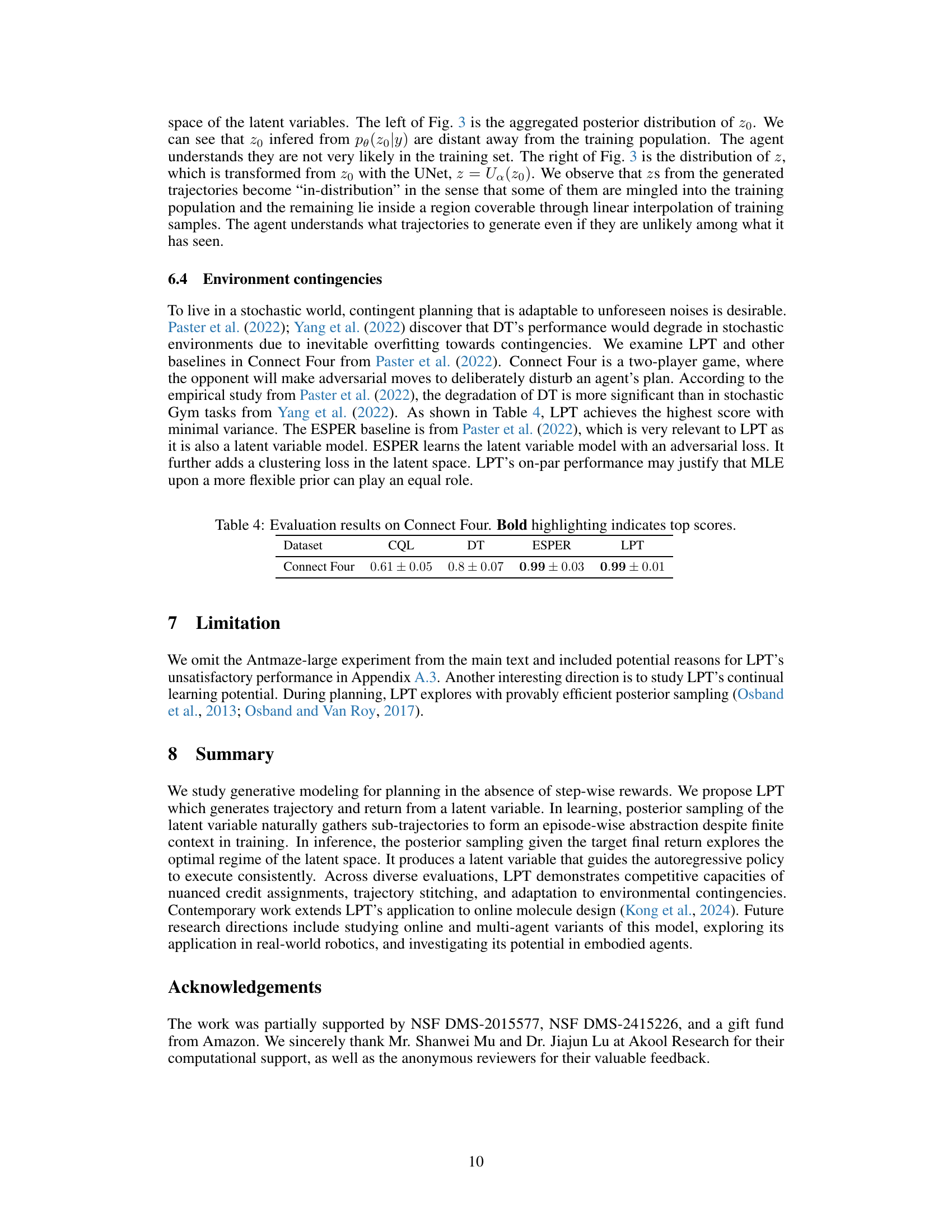
🔼 This table presents the performance comparison of different algorithms (CQL, DT, ESPER, and LPT) on the Connect Four game. The results are shown as mean ± standard deviation over 5 runs. The bold values highlight the best-performing algorithm for each metric, demonstrating LPT’s superior performance in this specific environment.
read the caption
Table 4: Evaluation results on Connect Four. Bold highlighting indicates top scores.

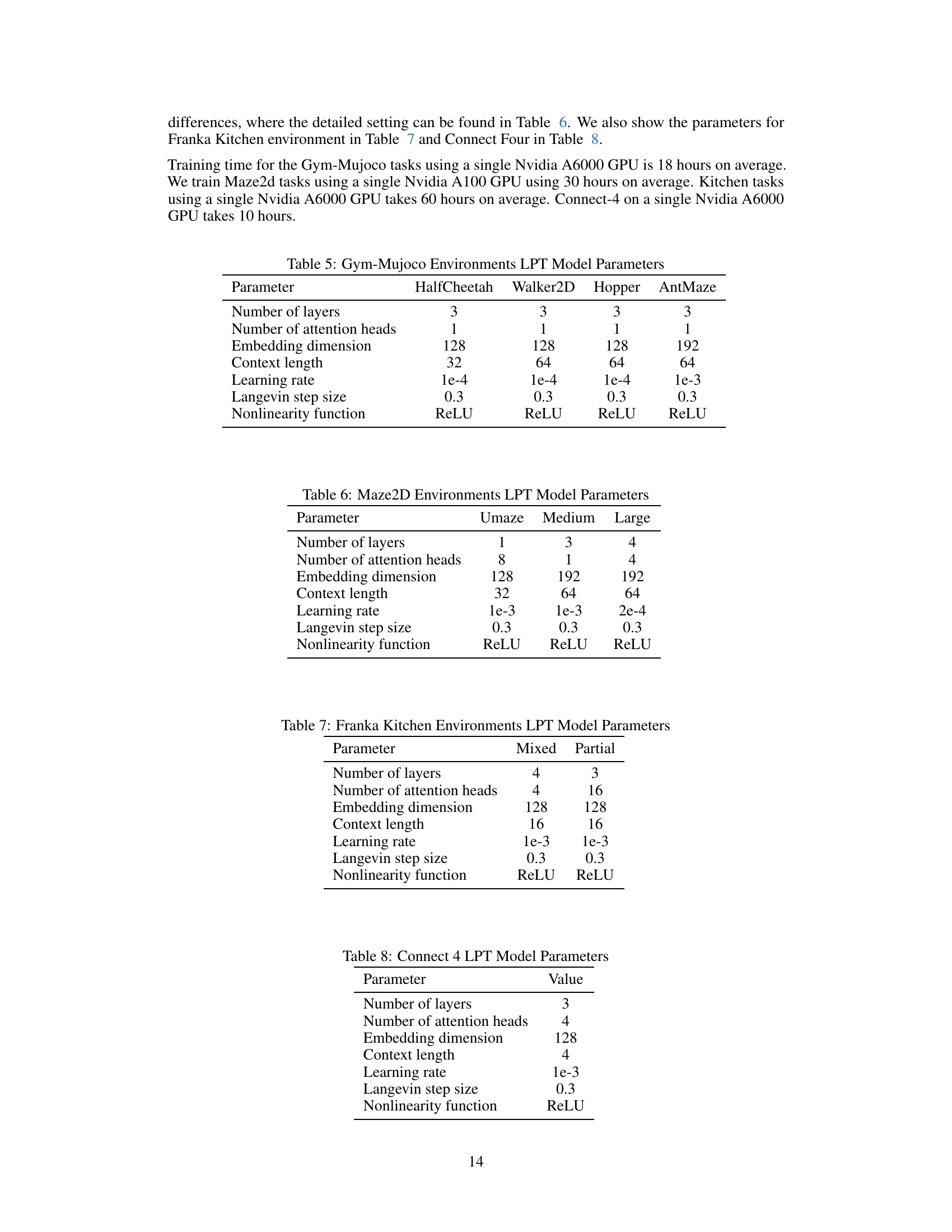
🔼 This table lists the hyperparameters used for training the Latent Plan Transformer (LPT) model on various Gym-Mujoco locomotion tasks. The parameters shown include the number of layers, attention heads, embedding dimension, context length, learning rate, Langevin step size, and the nonlinearity function used in the model architecture. These settings are task-specific, reflecting the differing complexities of the HalfCheetah, Walker2D, Hopper, and AntMaze environments.
read the caption
Table 5: Gym-Mujoco Environments LPT Model Parameters
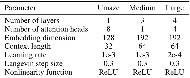
🔼 This table shows the hyperparameters used for training the Latent Plan Transformer (LPT) model on three different Maze2D environments: Umaze, Medium, and Large. Each environment has varying complexity, and these settings were adjusted to optimize performance for each environment’s unique characteristics. The parameters shown include the number of layers in the neural network, the number of attention heads used in the Transformer architecture, the embedding dimension, context length, learning rate, Langevin step size, and nonlinearity function.
read the caption
Table 6: Maze2D Environments LPT Model Parameters
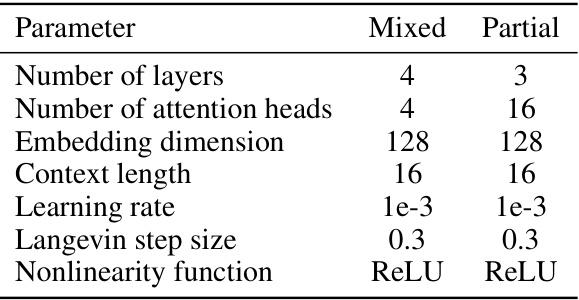
🔼 This table shows the hyperparameters used for training the Latent Plan Transformer (LPT) model on the Franka Kitchen dataset. It lists the number of layers, number of attention heads, embedding dimension, context length, learning rate, Langevin step size, and nonlinearity function used for both the ‘mixed’ and ‘partial’ datasets. The ‘mixed’ dataset contains both task-directed and non-task-directed demonstrations, while the ‘partial’ dataset contains primarily task-directed demonstrations. These parameters were adjusted to optimize the LPT model’s performance on the Franka Kitchen task.
read the caption
Table 7: Franka Kitchen Environments LPT Model Parameters

🔼 This table shows the hyperparameters used for the Connect 4 environment in the Latent Plan Transformer (LPT) model. It includes the number of layers, attention heads, embedding dimension, context length, learning rate, Langevin step size, and the nonlinearity function used.
read the caption
Table 8: Connect 4 LPT Model Parameters

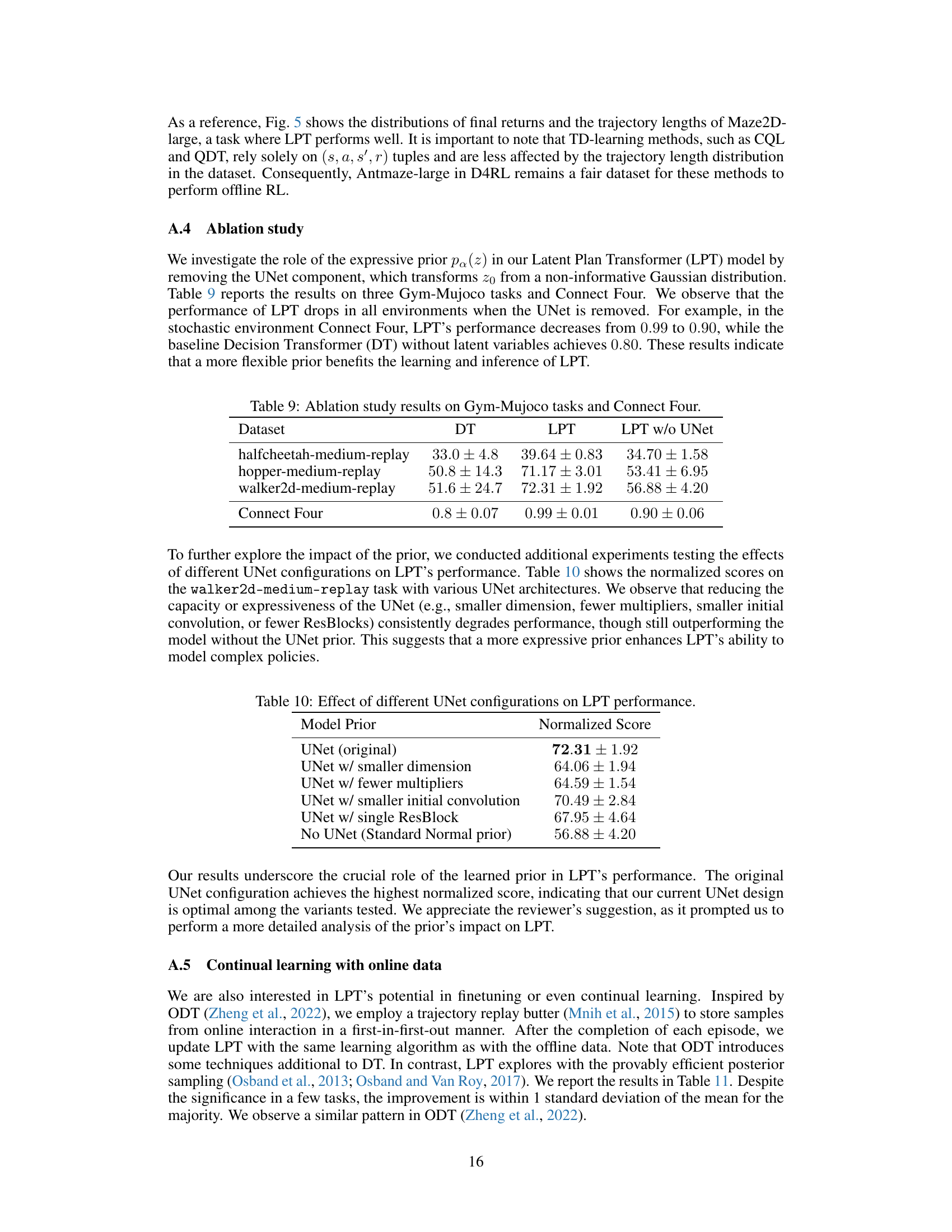
🔼 This table presents the results of an ablation study conducted to evaluate the impact of the expressive prior, specifically the UNet component, in the Latent Plan Transformer (LPT) model. By removing the UNet, the study assesses the model’s performance across three Gym-Mujoco tasks (halfcheetah-medium-replay, hopper-medium-replay, walker2d-medium-replay) and the Connect Four game. The results demonstrate a clear performance decrease across all tasks when the UNet is removed. The comparison includes scores for the original LPT model and a Decision Transformer (DT) baseline without latent variables.
read the caption
Table 9: Ablation study results on Gym-Mujoco tasks and Connect Four.

🔼 This ablation study investigates the impact of different UNet configurations on the LPT model’s performance. The table shows the normalized scores on the walker2d-medium-replay task using various UNet architectures, demonstrating that reducing the UNet’s capacity or expressiveness consistently degrades performance, highlighting the importance of a sufficiently expressive prior for enhanced model performance.
read the caption
Table 10: Effect of different UNet configurations on LPT performance.
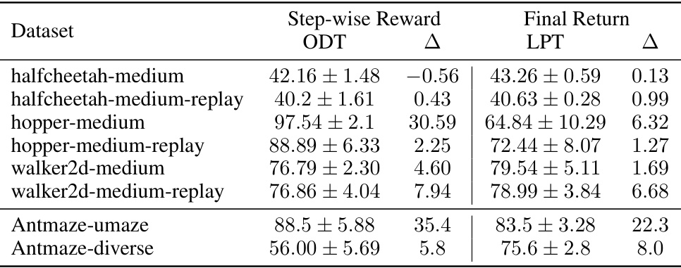
🔼 This table compares the performance of the proposed Latent Plan Transformer (LPT) model against the Decision Transformer (ODT) baseline on several online reinforcement learning tasks. The results show the average scores and standard deviations for both step-wise reward and final return settings, highlighting the improvement achieved by LPT in most tasks.
read the caption
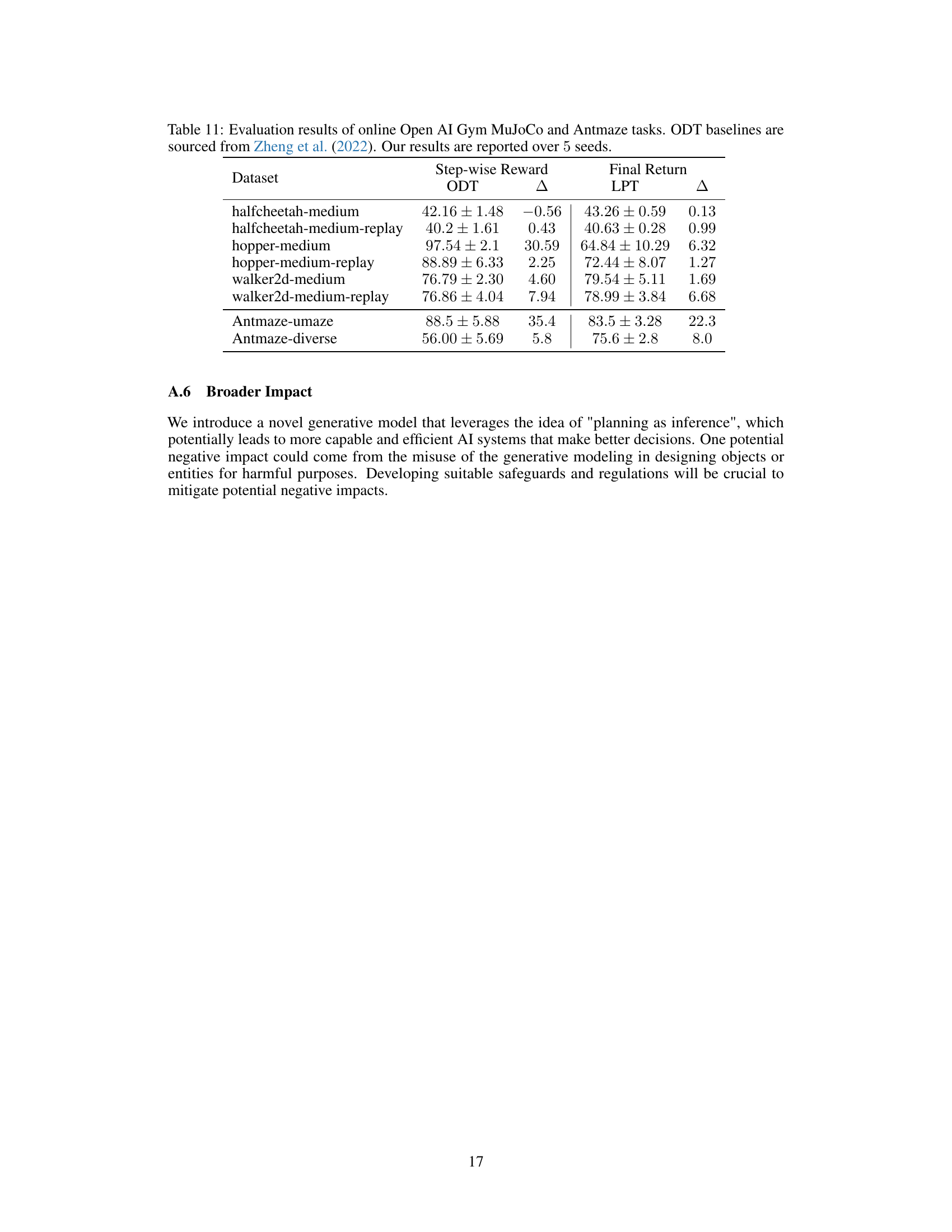
Table 11: Evaluation results of online OpenAI Gym MuJoCo and Antmaze tasks. ODT baselines are sourced from Zheng et al. (2022). Our results are reported over 5 seeds.
Full paper#

