TL;DR#
Large diffusion models, while powerful for image generation, are too large for many applications, especially those running on resource-constrained devices. Existing compression methods often compromise generation quality or only achieve modest compression. This creates a significant hurdle for wider adoption of these models.
BitsFusion overcomes these challenges with a novel mixed-precision weight quantization method that compresses the UNet of Stable Diffusion v1.5 to 1.99 bits, resulting in a 7.9x size reduction. The technique involves assigning optimal bit-widths to each layer based on an analysis of quantization error, using carefully designed initialization strategies, and employing a two-stage training pipeline. Importantly, BitsFusion achieves better generation quality than the original model, demonstrating significant advancement in model compression without sacrificing performance.
Key Takeaways#
Why does it matter?#
This paper is significant because it presents BitsFusion, a novel method for drastically reducing the size of large diffusion models. This is crucial for deploying these models on resource-constrained devices and making them more accessible for a wider range of applications. The high compression ratio (7.9x) achieved while maintaining or improving image quality opens exciting new avenues for research in model compression and efficient AI.
Visual Insights#

🔼 This figure displays a comparison of images generated using the full-precision Stable Diffusion v1.5 model and the BitsFusion model (with UNet weights quantized to 1.99 bits). The top row shows images from the full-precision model, while the bottom row shows images generated by BitsFusion. The significant reduction in model size (7.9x) is achieved with comparable image quality. All images were generated using the same parameters (PNDM sampler, 50 sampling steps, random seed 1024), differing only in the model used.
read the caption
Figure 1: Top: Images generated from full-precision Stable Diffusion v1.5. Bottom: Images generated from BitsFusion, where the weights of UNet are quantized into 1.99 bits, achieving 7.9× smaller storage than the one from Stable Diffusion v1.5. All the images are synthesized under the setting of using PNDM sampler [49] with 50 sampling steps and random seed as 1024. Prompts and more generations are provided in App. M.

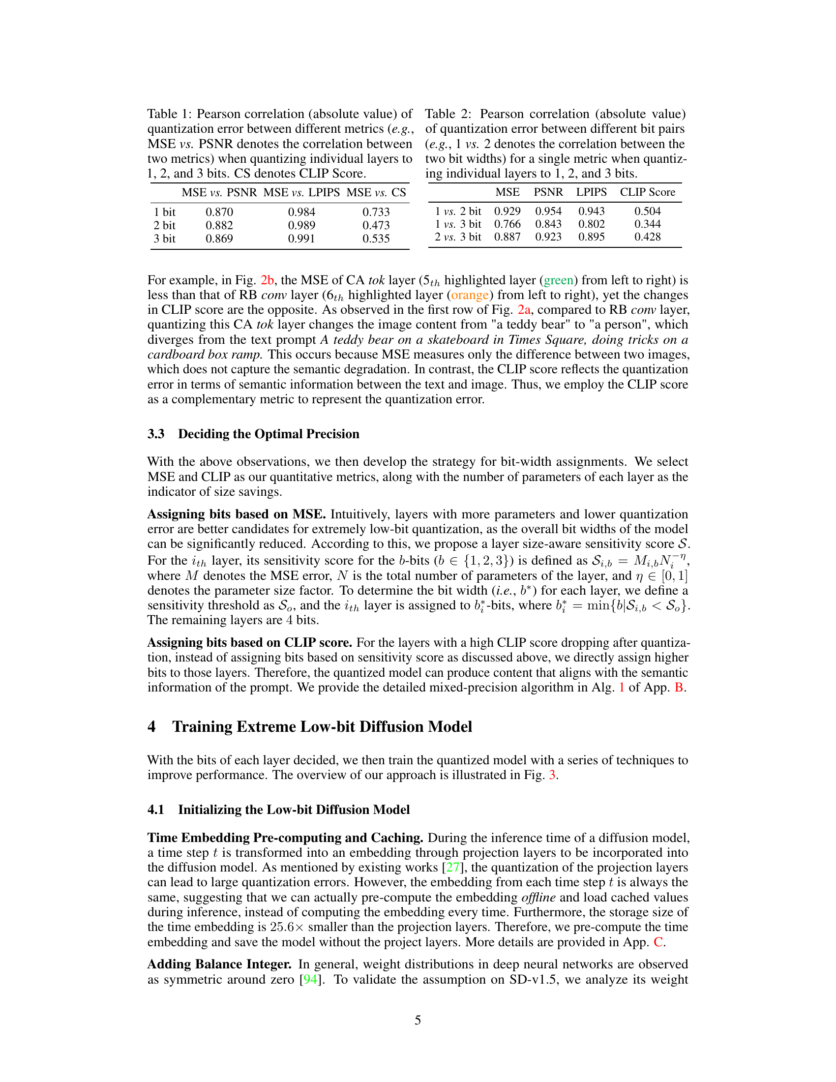
🔼 This table presents the Pearson correlation coefficients between different image quality metrics (MSE, PSNR, LPIPS, and CLIP Score) when individual layers of a Stable Diffusion model are quantized to 1, 2, or 3 bits. It shows the strength of the linear relationship between pairs of metrics across different quantization levels. A high correlation suggests that these metrics capture similar aspects of image quality degradation caused by quantization.
read the caption
Table 1: Pearson correlation (absolute value) of quantization error between different metrics (e.g., MSE vs. PSNR denotes the correlation between two metrics) when quantizing individual layers to 1, 2, and 3 bits. CS denotes CLIP Score.
In-depth insights#
Quantization Methods#
In exploring the realm of ‘Quantization Methods’ within the context of a research paper, several key aspects warrant in-depth analysis. Post-training quantization (PTQ) techniques, which involve quantizing pre-trained models without retraining, are attractive for their efficiency. However, they often suffer from performance degradation compared to quantization-aware training. Quantization-aware training (QAT) methods, on the other hand, incorporate quantization constraints into the training process, leading to superior performance but increased computational cost. A critical factor is the choice of quantization bit-width, with lower bit-widths resulting in smaller models but potentially sacrificing accuracy. The paper should explore various bit-widths and analyze the trade-off between model size and performance. Mixed-precision quantization, where different layers of a model are quantized with different bit-widths, provides a nuanced approach that balances model compression and accuracy. The effectiveness of any quantization method heavily depends on the architecture of the underlying model. Careful consideration of layer-wise quantization sensitivity is crucial for optimizing the overall performance. Advanced techniques, such as the use of scaling factors, zero-point adjustments, and novel training strategies designed to address the quantization error, should also be discussed. Finally, a robust evaluation comparing several quantization strategies across various metrics is essential, ideally including both quantitative and qualitative measures of generation quality.
Mixed Precision#
The concept of “mixed precision” in numerical computation, particularly within the context of deep learning, involves using different levels of precision (e.g., FP16, FP32, INT8) for various parts of a model or algorithm. This strategy is driven by the trade-off between computational efficiency and numerical accuracy. Lower precision formats, such as FP16 or INT8, offer significant speedups and reduced memory footprint during training and inference, but can lead to numerical instability or reduced accuracy if not managed carefully. A well-designed mixed-precision scheme aims to utilize higher precision where necessary to maintain numerical stability in critical operations, while employing lower precision for less sensitive parts to improve efficiency. Careful consideration is required in selecting which parts of the model will benefit most from the speed improvement of lower precision and determining how to avoid the pitfalls of lower precision. This selection often depends on empirical analysis and the specific characteristics of the model and the training process. The success of a mixed-precision approach relies heavily on its ability to balance the need for accuracy with the desire for efficiency. It often involves techniques like loss scaling to alleviate the effects of reduced precision, careful initialization, and potentially specialized training algorithms.
Training Strategies#
Effective training strategies are crucial for successful model development, especially when dealing with complex architectures and limited resources. A thoughtful approach to training would likely involve a multi-stage training process, perhaps starting with a distillation phase, where a smaller, quantized model learns from a larger, high-precision model. This strategy can effectively transfer knowledge and improve the efficiency of training the smaller model. The subsequent stages might focus on fine-tuning to optimize the quantized model’s performance on the target task, potentially using techniques such as curriculum learning to gradually increase the difficulty of the training data. Another key aspect is optimization of hyperparameters, which can significantly influence model performance. Careful selection and tuning of the hyperparameters, perhaps using techniques like Bayesian optimization or evolutionary strategies, is crucial to finding the optimal training configuration. The final stage may involve evaluation and refinement based on comprehensive metrics, ensuring the model meets the desired performance standards.
Ablation Study#
An ablation study systematically evaluates the contribution of individual components within a machine learning model. In the context of a research paper, a well-executed ablation study would dissect a complex model, removing or altering single parts (e.g., specific layers, modules, or hyperparameters) to observe the impact on performance. The goal is to isolate and quantify the effect of each component, clarifying its importance and guiding future model design or optimization efforts. A strong ablation study will follow a rigorous methodology, carefully controlling for confounding variables to ensure that observed changes are attributable to the modification and not extraneous factors. Results are often presented visually, using graphs or tables to showcase the relative contributions of different components, enhancing the reader’s understanding of the model’s inner workings. A well-designed ablation study strengthens a paper’s overall contribution by providing empirical evidence supporting the authors’ claims about the model’s architecture and its effectiveness.
Future Work#
The ‘Future Work’ section of a research paper on low-bit quantization of diffusion models could explore several promising avenues. Extending the quantization techniques to other components of the diffusion model, beyond the UNet, such as the VAE or text encoder, could significantly improve overall model efficiency. Investigating alternative quantization methods, like learned quantization or non-uniform quantization, could lead to better performance compared to uniform quantization. Developing more sophisticated training strategies for low-bit models, such as improved distillation techniques or exploration of novel training loss functions, would be beneficial. Further analysis of quantization effects on specific layers and how to optimize bit allocation to further minimize the overall quantization error warrants investigation. A comprehensive evaluation of the proposed model on broader tasks and datasets would provide stronger evidence of its generalizability and robustness. Finally, exploring the application of low-bit quantization to other types of generative models or even exploring this work in combination with other compression techniques like pruning, could expand the impact of this research significantly.
More visual insights#
More on figures

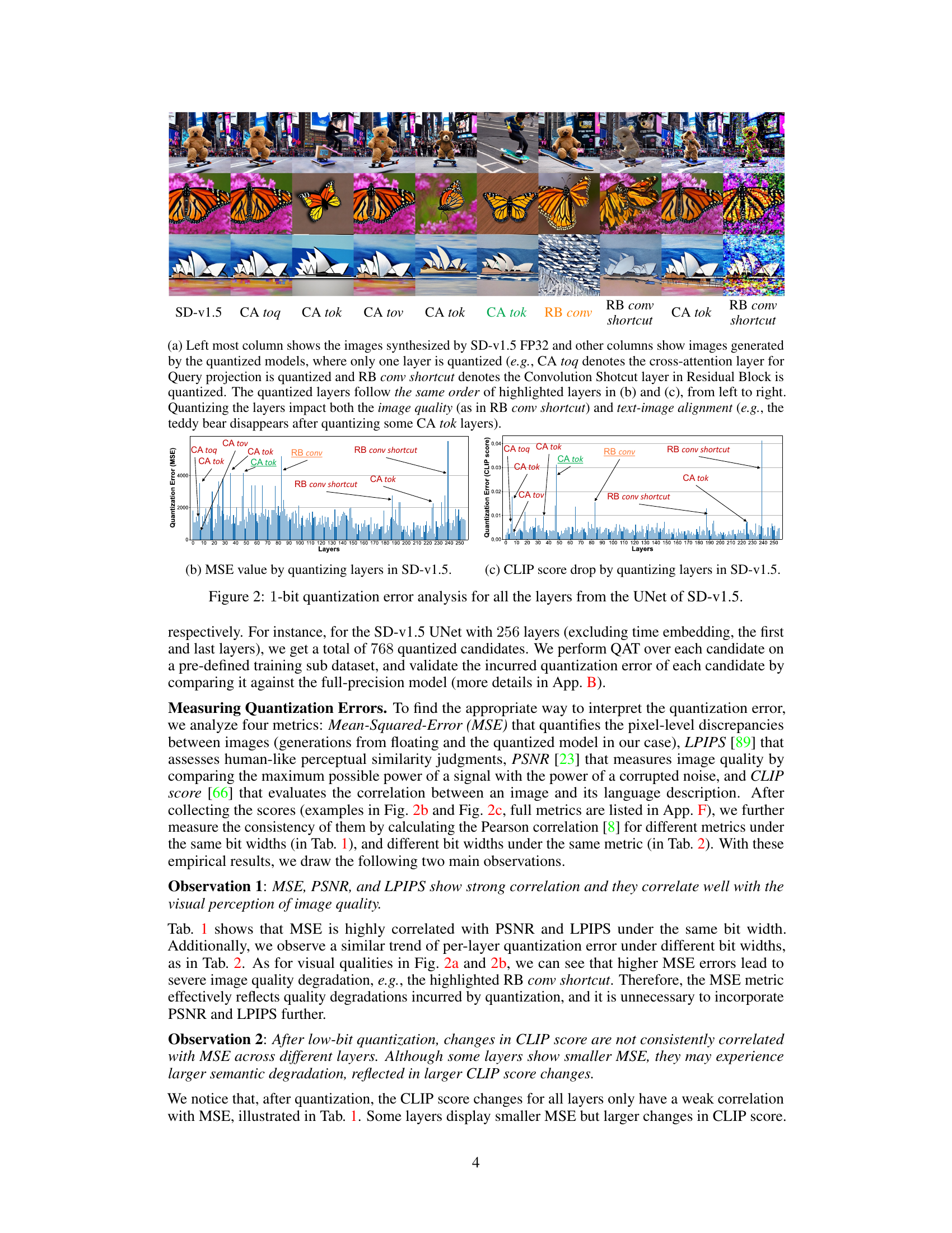
🔼 This figure presents a per-layer sensitivity analysis of the Stable Diffusion v1.5 UNet model. Each subfigure shows the results of quantizing individual layers to 1 bit while keeping other layers at full precision. (a) shows the images generated with only one layer quantized to 1-bit at a time, demonstrating the impact on image quality and text-image alignment. (b) and (c) provide line graphs showing the Mean Squared Error (MSE) and CLIP score drop, respectively, for each layer when quantized to 1-bit. These graphs help illustrate which layers are most sensitive to 1-bit quantization and inform the mixed-precision quantization strategy.
read the caption
Figure 2: 1-bit quantization error analysis for all the layers from the UNet of SD-v1.5.

🔼 This figure shows the results of a per-layer sensitivity analysis conducted on the Stable Diffusion v1.5 UNet model. Each layer was quantized to 1 bit individually while keeping other layers at full precision. The analysis measured the impact on image generation quality using MSE (Mean Squared Error) and CLIP score (a metric of text-image alignment). The figure displays two graphs, one showing the MSE value for each layer after 1-bit quantization and another showing the change in CLIP score for each layer. This analysis helps determine which layers are more sensitive to quantization and guides the selection of optimal bit-widths in a mixed-precision quantization strategy.
read the caption
Figure 2: 1-bit quantization error analysis for all the layers from the UNet of SD-v1.5.

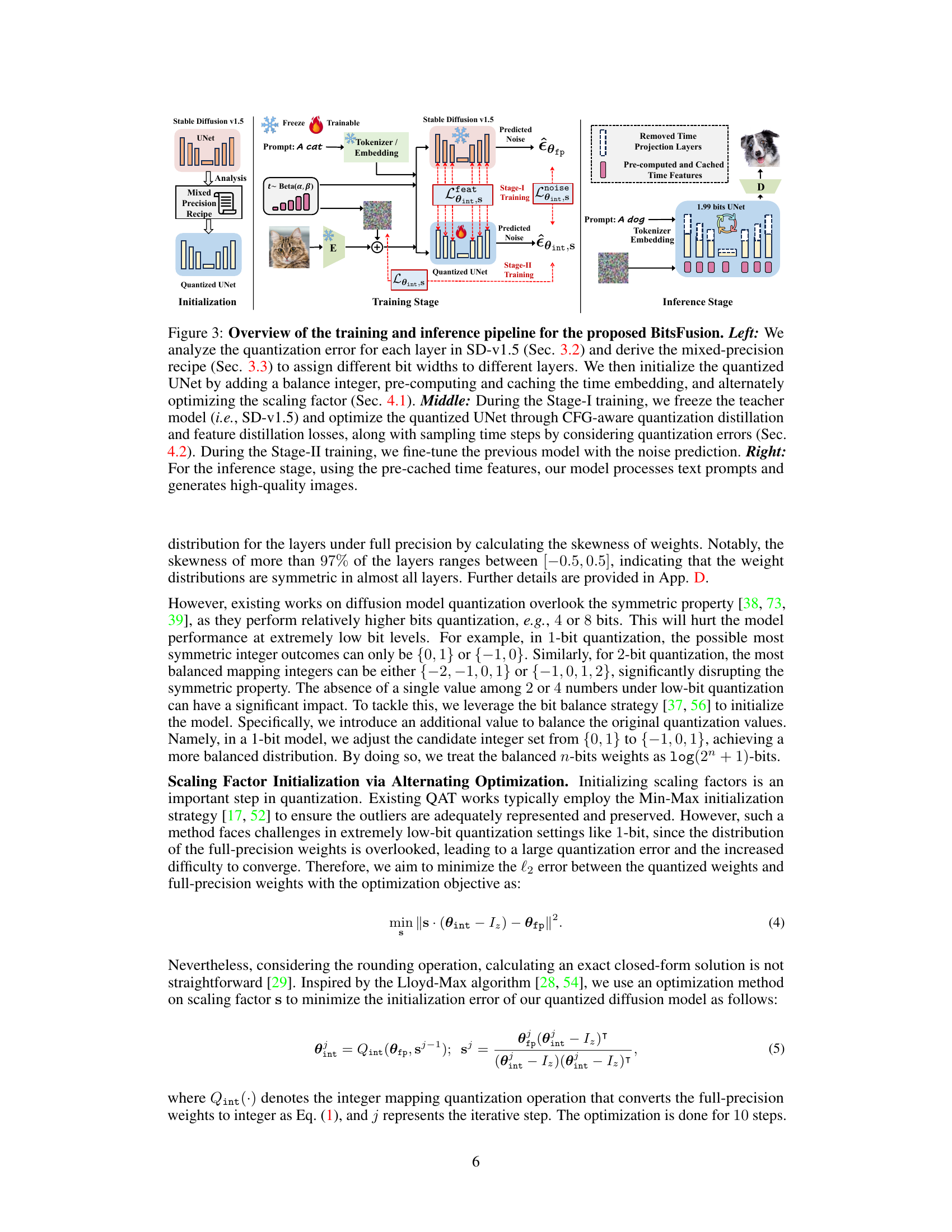
🔼 This figure illustrates the training and inference pipeline of BitsFusion. The left part shows the analysis of quantization error, the derivation of mixed-precision recipe, and initialization of the quantized UNet. The middle part describes the two-stage training process: Stage-I utilizes CFG-aware quantization distillation and feature distillation, while Stage-II fine-tunes the model using noise prediction. The right part shows the inference stage using pre-computed time features to generate images.
read the caption
Figure 3: Overview of the training and inference pipeline for the proposed BitsFusion. Left: We analyze the quantization error for each layer in SD-v1.5 (Sec. 3.2) and derive the mixed-precision recipe (Sec. 3.3) to assign different bit widths to different layers. We then initialize the quantized UNet by adding a balance integer, pre-computing and caching the time embedding, and alternately optimizing the scaling factor (Sec. 4.1). Middle: During the Stage-I training, we freeze the teacher model (i.e., SD-v1.5) and optimize the quantized UNet through CFG-aware quantization distillation and feature distillation losses, along with sampling time steps by considering quantization errors (Sec. 4.2). During the Stage-II training, we fine-tune the previous model with the noise prediction. Right: For the inference stage, using the pre-cached time features, our model processes text prompts and generates high-quality images.
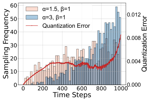
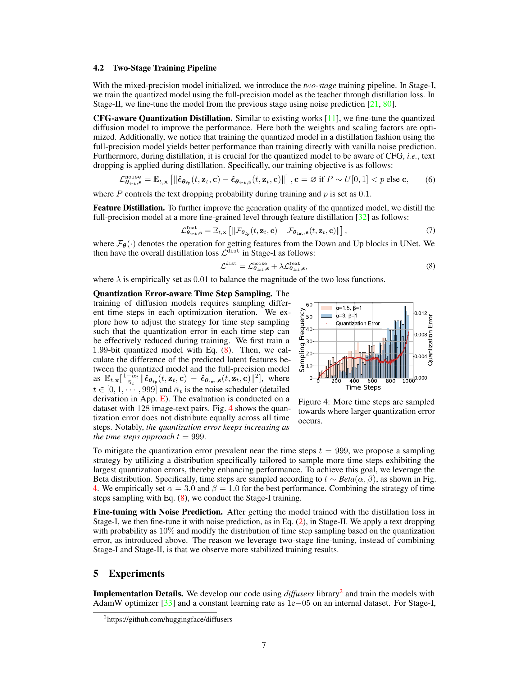
🔼 This figure shows the relationship between the quantization error and the sampling frequency of different time steps during the training of a 1.99-bit quantized diffusion model. The x-axis represents the time steps, ranging from 0 to 999. The left y-axis shows the sampling frequency, illustrating how often each time step is sampled during training. Two different beta distributions (α=1.5, β=1 and α=3, β=1) are shown to demonstrate how adjusting these parameters affects the sampling distribution. The right y-axis shows the quantization error for each time step, represented by a red line. The figure demonstrates that by adjusting the beta distribution parameters (specifically using α=3, β=1), more time steps with higher quantization errors are sampled more frequently during training, which helps to mitigate the impact of these high-error steps.
read the caption
Figure 4: More time steps are sampled towards where larger quantization error occurs.

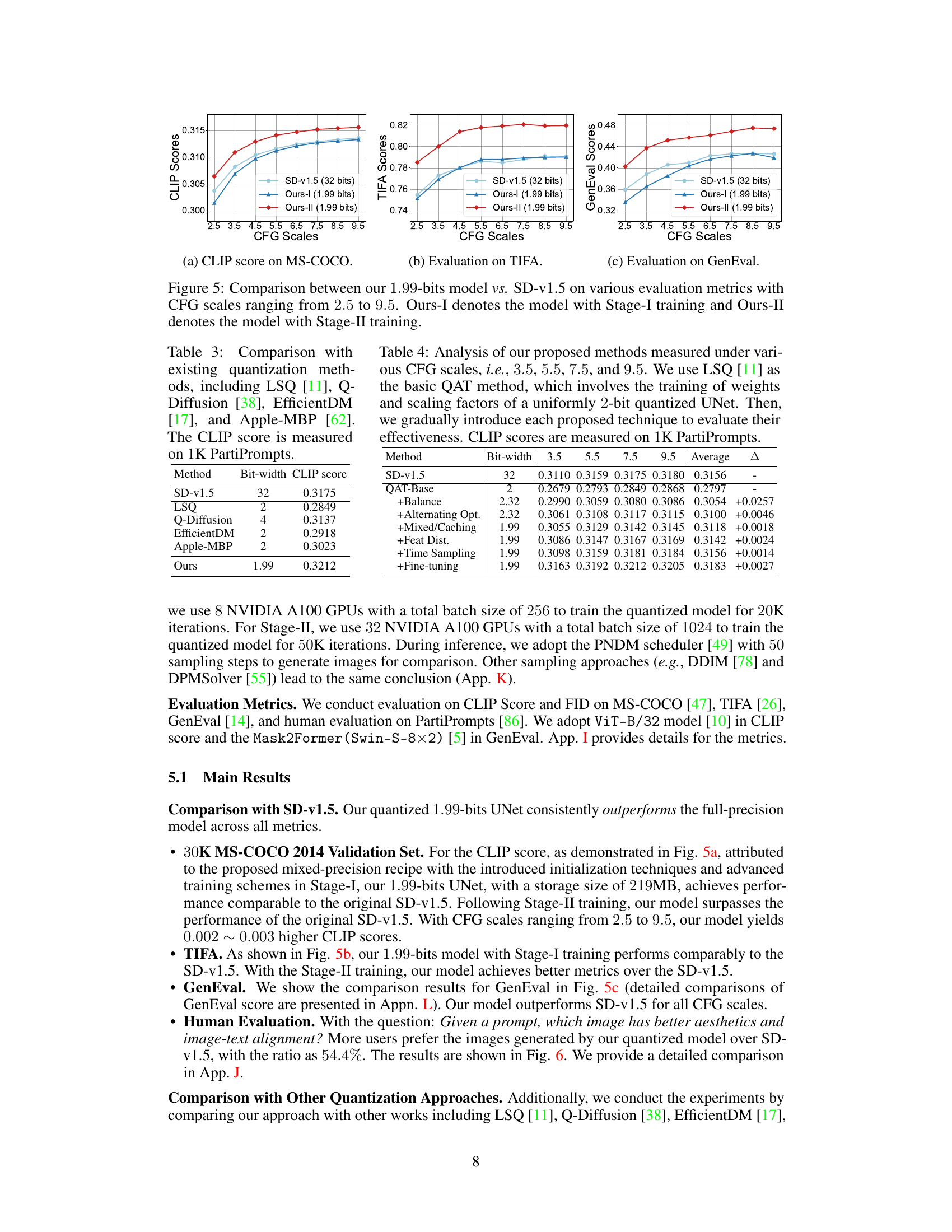
🔼 This figure shows the performance comparison between the proposed 1.99-bit quantized model (BitsFusion) and the original Stable Diffusion v1.5 (SD-v1.5) across three different evaluation metrics: CLIP score, TIFA score, and GenEval score. The comparison is made for various CFG (Classifier-Free Guidance) scales, ranging from 2.5 to 9.5. The results indicate that BitsFusion, especially after Stage-II training, consistently outperforms SD-v1.5 across all metrics and CFG scales.
read the caption
Figure 5: Comparison between our 1.99-bits model vs. SD-v1.5 on various evaluation metrics with CFG scales ranging from 2.5 to 9.5. Ours-I denotes the model with Stage-I training and Ours-II denotes the model with Stage-II training.
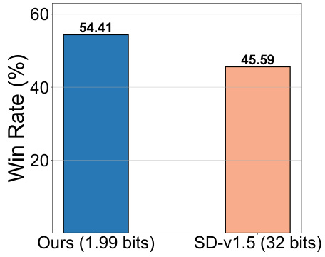
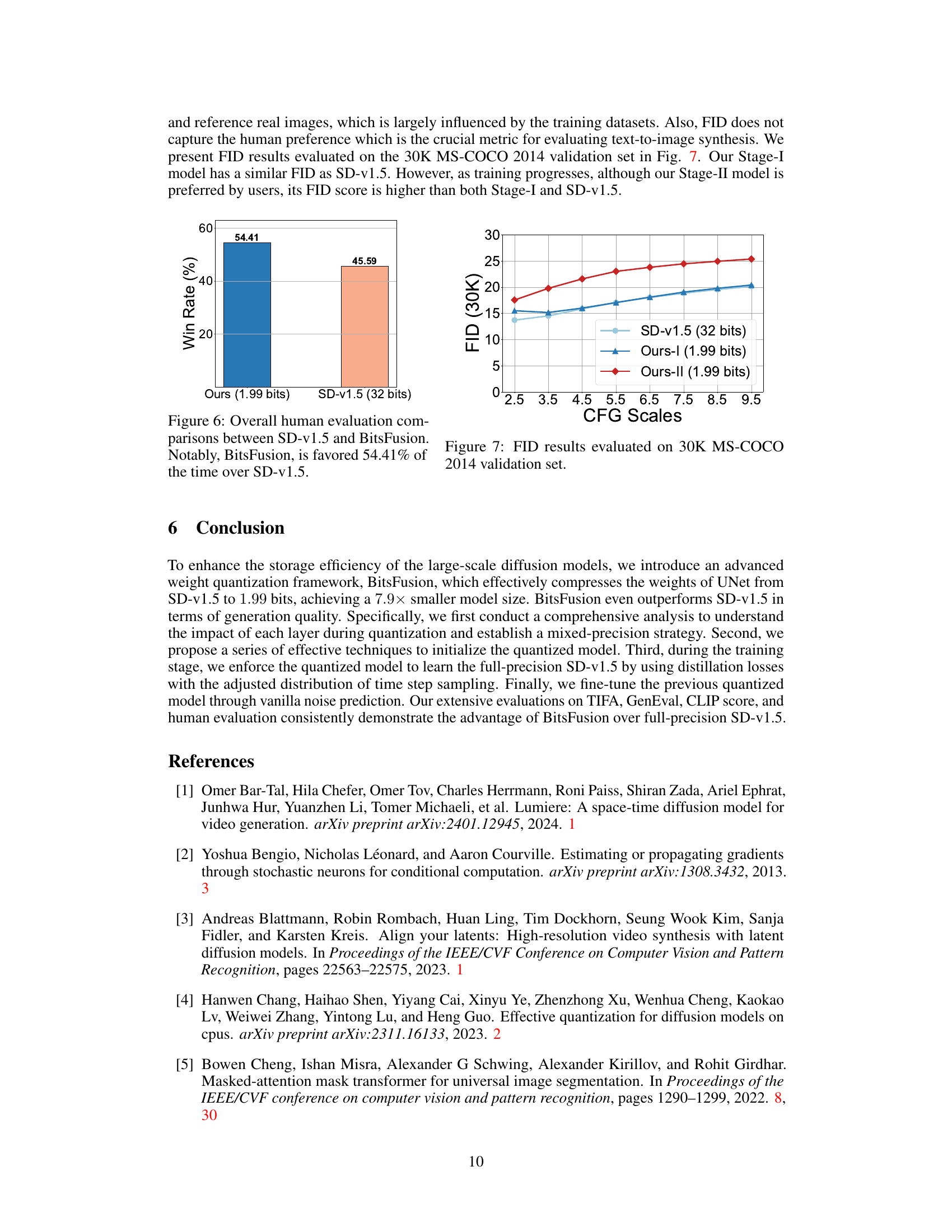
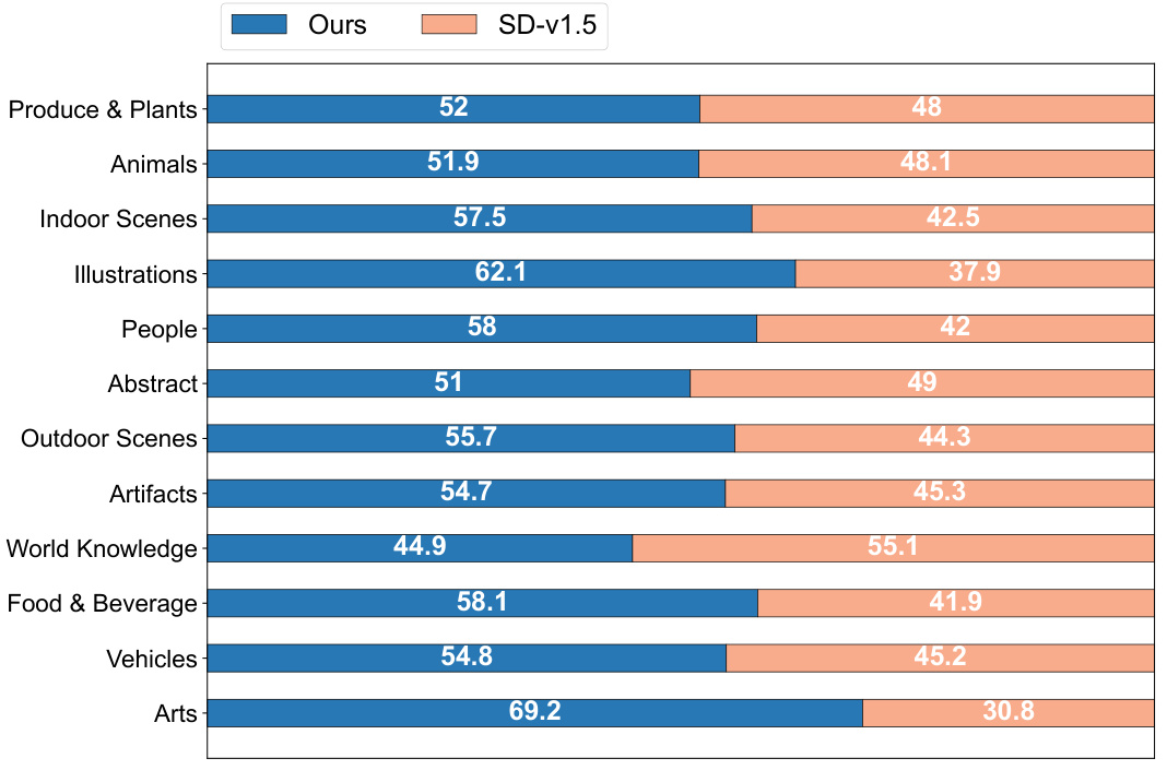
🔼 This figure shows the results of a human evaluation comparing the image generation quality of the proposed BitsFusion model (1.99 bits) against the original Stable Diffusion v1.5 (32 bits). The evaluation focused on user preference, showing that 54.41% of the time, participants preferred images generated by the quantized BitsFusion model. This demonstrates the superior performance of the quantized model, despite its significantly smaller size.
read the caption
Figure 6: Overall human evaluation comparisons between SD-v1.5 and BitsFusion. Notably, BitsFusion is favored 54.41% of the time over SD-v1.5.
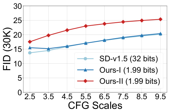
🔼 This figure compares the performance of the proposed 1.99-bit quantized model (BitsFusion) against the original Stable Diffusion v1.5 (SD-v1.5) across three different evaluation metrics: CLIP score, TIFA score, and GenEval score. The comparison is performed at various CFG (Classifier-Free Guidance) scales, ranging from 2.5 to 9.5. The results show that the quantized model, especially after the second stage of training, consistently outperforms or matches the full-precision model across all metrics and CFG scales.
read the caption
Figure 5: Comparison between our 1.99-bits model vs. SD-v1.5 on various evaluation metrics with CFG scales ranging from 2.5 to 9.5. Ours-I denotes the model with Stage-I training and Ours-II denotes the model with Stage-II training.

🔼 This figure presents a per-layer sensitivity analysis of the Stable Diffusion v1.5 UNet model. Each subfigure shows the quantization error after quantizing a single layer to 1 bit while keeping other layers at full precision. Subfigure (a) shows images generated under different quantization settings, illustrating the impact on visual quality. Subfigures (b) and (c) depict the MSE and CLIP score changes respectively, showing how different layers’ quantization affect the overall results. This analysis informs the mixed-precision quantization strategy of the BitsFusion model.
read the caption
Figure 2: 1-bit quantization error analysis for all the layers from the UNet of SD-v1.5.
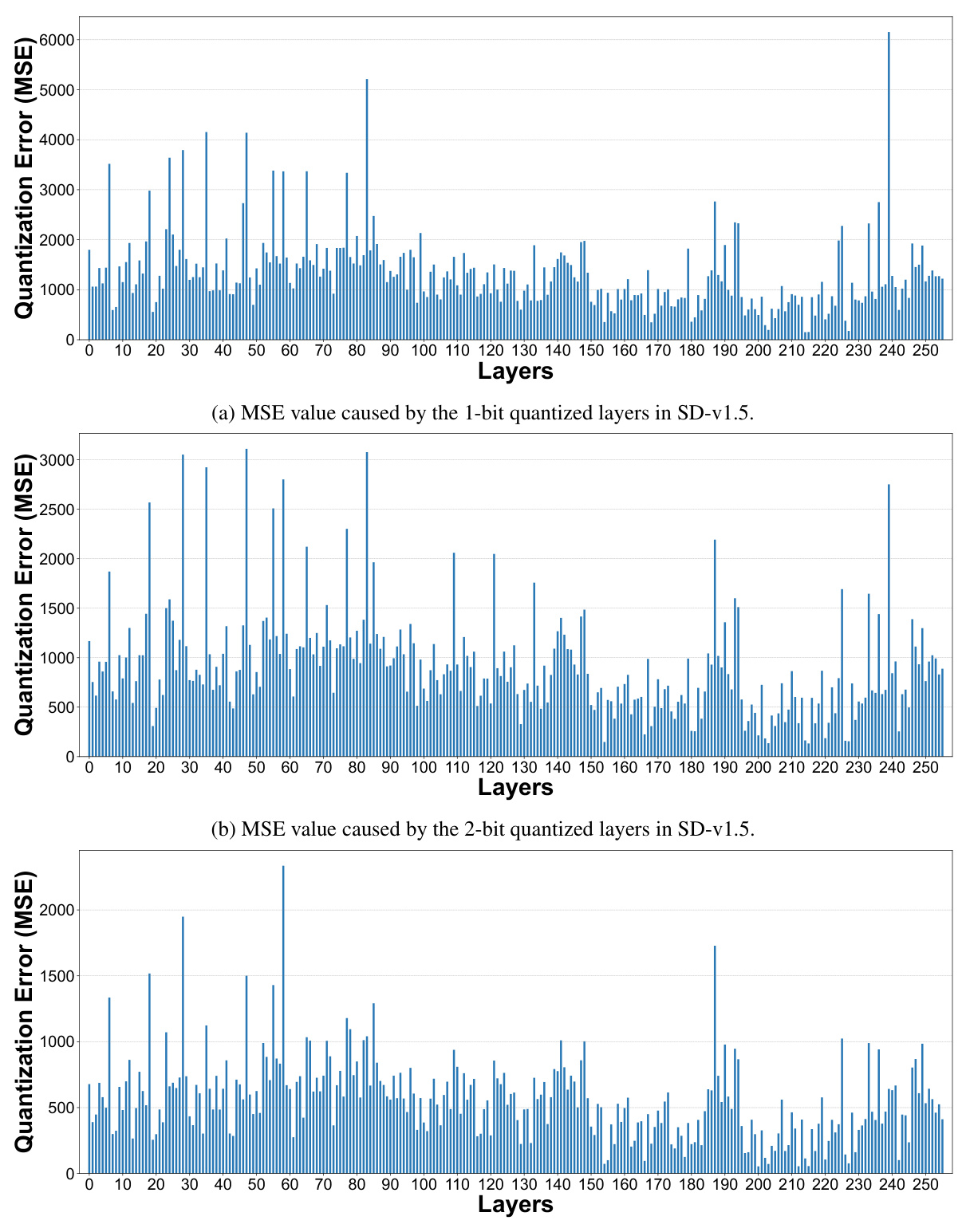
🔼 This figure presents a per-layer sensitivity analysis of the Stable Diffusion v1.5 UNet model by quantizing each layer to 1, 2, and 3 bits while freezing others at full precision. It shows the quantization error for each layer using Mean Squared Error (MSE) and CLIP score. (a) shows the MSE values for each layer quantized to 1 bit, (b) shows the MSE values for each layer quantized to 2 bits, and (c) shows the CLIP score drop for each layer quantized to 1, 2, and 3 bits. The analysis helps determine the optimal bit-width assignment for each layer in a mixed-precision quantization strategy. The results illustrate how different layers exhibit varying sensitivities to quantization, informing the optimal bit assignment for each layer, aiming to minimize the overall quantization error while maximizing size reduction.
read the caption
Figure 2: 1-bit quantization error analysis for all the layers from the UNet of SD-v1.5.
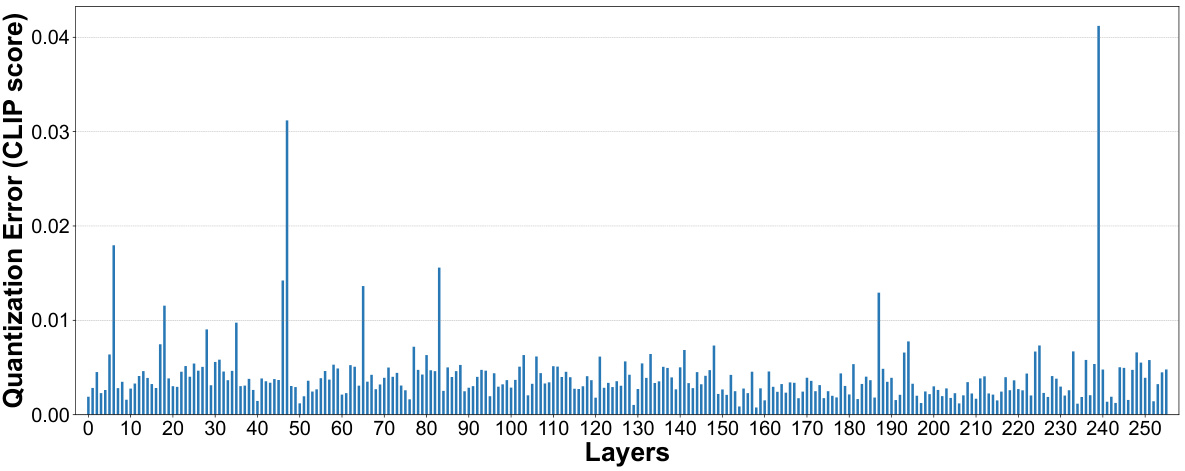
🔼 This figure presents a per-layer sensitivity analysis of the Stable Diffusion v1.5 UNet model, quantizing each layer to 1, 2, and 3 bits individually while keeping others at full precision. Subsequently, quantization-aware training (QAT) was performed on each layer. The results are visualized to show the quantization error (MSE and CLIP score) for each layer at different bit depths. The purpose is to determine the sensitivity of different layers to quantization and inform a mixed-precision quantization strategy where different layers are quantized to different bit-depths based on their error profiles. (a) shows MSE values, (b) shows CLIP score drops.
read the caption
Figure 2: 1-bit quantization error analysis for all the layers from the UNet of SD-v1.5.
🔼 This figure presents a per-layer sensitivity analysis of the Stable Diffusion v1.5 UNet model. Each subfigure visualizes the quantization error for a different aspect when each layer is quantized to 1 bit while others remain at full precision. (a) shows the Mean Squared Error (MSE) for each layer. (b) shows the change in CLIP score (a measure of text-image alignment) for each layer. (c) shows the combination of both MSE and CLIP score to illustrate how different layers are sensitive to quantization. The figure is used to inform the mixed-precision quantization strategy adopted in the paper.
read the caption
Figure 2: 1-bit quantization error analysis for all the layers from the UNet of SD-v1.5.

🔼 This figure presents the results of a per-layer sensitivity analysis performed on the UNet of Stable Diffusion v1.5. Each layer was quantized to 1 bit, while the rest of the network remained at full precision. The analysis evaluated the impact of this quantization on various metrics, including Mean Squared Error (MSE), which measures pixel-level differences, and CLIP score, which assesses the alignment between image content and text prompts. The figure shows plots illustrating the MSE value and CLIP score drop for each layer after 1-bit quantization. This analysis informs the selection of optimal bit widths for each layer in a mixed-precision quantization strategy.
read the caption
Figure 2: 1-bit quantization error analysis for all the layers from the UNet of SD-v1.5.

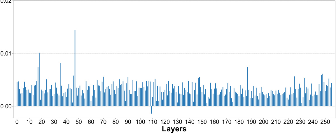
🔼 This figure shows the LPIPS (Learned Perceptual Image Patch Similarity) values for each layer of the Stable Diffusion v1.5 (SD-v1.5) model after applying 1-bit, 2-bit, and 3-bit quantization. LPIPS is a metric that measures the perceptual similarity between images. Lower LPIPS values indicate higher visual similarity between the original and quantized images. The figure helps in analyzing the impact of quantization on the perceptual quality of images generated by different layers of the model. Each sub-figure (a), (b), and (c) represents the results for 1-bit, 2-bit, and 3-bit quantization, respectively, providing a visual representation of the per-layer quantization error in terms of perceptual quality.
read the caption
Figure 11: LPIPS value of quantized layers in SD-v1.5.

🔼 This figure shows the LPIPS (Learned Perceptual Image Patch Similarity) values for each layer of the Stable Diffusion v1.5 (SD-v1.5) model after applying different levels of quantization (1-bit, 2-bit, and 3-bit). LPIPS is a metric that measures the perceptual similarity between images, so lower LPIPS values indicate less visual degradation due to quantization. The figure helps to demonstrate the impact of quantization on different layers, providing data to support the decision-making for which layers should be quantized more aggressively and which should be given more precision.
read the caption
Figure 11: LPIPS value of quantized layers in SD-v1.5.

🔼 This figure presents a per-layer sensitivity analysis of the Stable Diffusion v1.5 UNet model. Each subfigure shows the impact of quantizing individual layers to 1 bit on various metrics: (a) Mean Squared Error (MSE), (b) change in CLIP score, and (c) change in perceptual similarity metrics (LPIPS). The x-axis represents the layer number, and the y-axis shows the error. This analysis helps to understand which layers are more sensitive to quantization and informs the mixed-precision quantization strategy where different layers are assigned different bit depths depending on their sensitivity.
read the caption
Figure 2: 1-bit quantization error analysis for all the layers from the UNet of SD-v1.5.
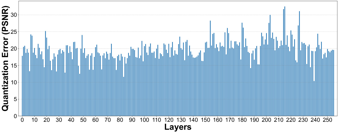
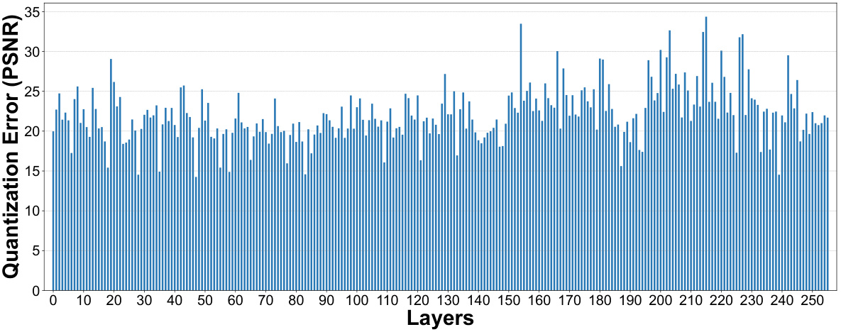
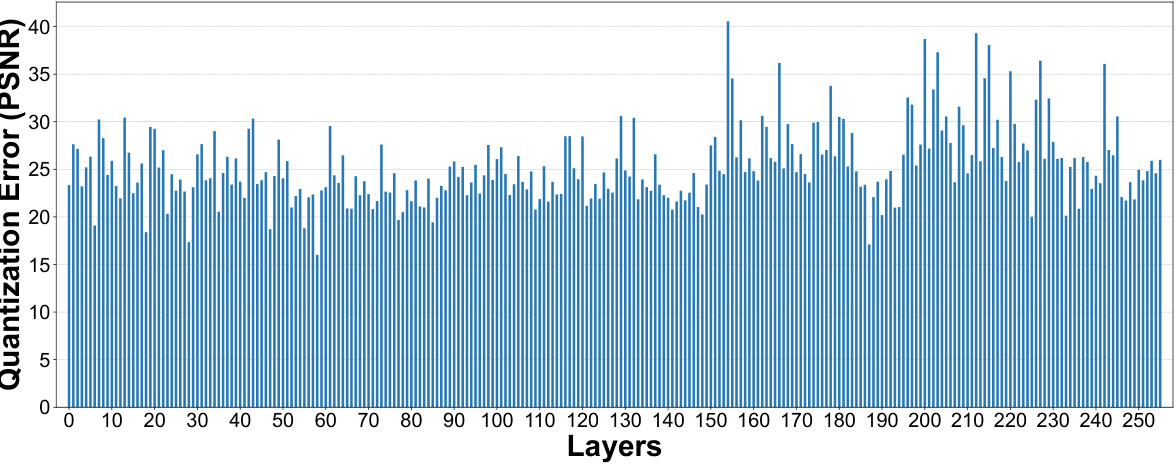
🔼 This figure shows the PSNR values of quantized layers in Stable Diffusion v1.5 for 1-bit, 2-bit, and 3-bit quantization. The x-axis represents the layer number, while the y-axis represents the PSNR value. The figure illustrates the quantization error per layer for different quantization bit-widths, showing the impact of quantization on image quality layer by layer.
read the caption
Figure 12: PSNR value of quantized layers in SD-v1.5.
🔼 This figure shows the mean squared error (MSE) values for each layer of the Stable Diffusion v1.5 model when quantized to 1, 2, and 3 bits. The x-axis represents the layer number (out of 256), and the y-axis represents the MSE value. Each subplot shows the MSE for a different bit quantization level. This helps to visualize the impact of quantization on different layers of the model, allowing for the selection of an optimal quantization strategy by assigning different bit widths to various layers.
read the caption
Figure 9: MSE value caused by the quantized layers in SD-v1.5.
🔼 This figure shows the results of a per-layer sensitivity analysis performed on the Stable Diffusion v1.5 UNet model. Each layer was quantized to 1 bit while keeping the rest at full precision. Quantization-aware training was performed, and the quantization error was evaluated using MSE and CLIP score. Subfigure (a) shows example images generated from quantizing a single layer to illustrate that different layers have different impacts on generation quality and text-image alignment. Subfigures (b) and (c) show the MSE and CLIP score drop for each layer respectively, showing the distribution of quantization error across all layers. This analysis informs the mixed-precision quantization strategy used in the paper.
read the caption
Figure 2: 1-bit quantization error analysis for all the layers from the UNet of SD-v1.5.

🔼 This figure shows a comparison between images generated by the full-precision Stable Diffusion v1.5 and the quantized model (BitsFusion). Six different prompts were used to generate pairs of images. The top row shows the images generated by Stable Diffusion, and the bottom row shows the images generated by BitsFusion, demonstrating the quantized model’s ability to produce high-quality images comparable to the full-precision model.
read the caption
Figure 17: Top: Images generated from full-precision Stable Diffusion v1.5. Bottom: Images generated from BitsFusion. Prompts from left to right are: a: A person standing on the desert, desert waves, gossip illustration, half red, half blue, abstract image of sand, clear style, trendy illustration, outdoor, top view, clear style, precision art, ultra high definition image; b: A detailed oil painting of an old sea captain, steering his ship through a storm. Saltwater is splashing against his weathered face, determination in his eyes. Twirling malevolent clouds are seen above and stern waves threaten to submerge the ship while seagulls dive and twirl through the chaotic landscape. Thunder and lights embark in the distance, illuminating the scene with an eerie green glow.; c: A solitary figure shrouded in mists peers up from the cobble stone street at the imposing and dark gothic buildings surrounding it. an old-fashioned lamp shines nearby. oil painting.; d: A deep forest clearing with a mirrored pond reflecting a galaxy-filled night sky; e: a handsome 24 years old boy in the middle with sky color background wearing eye glasses, it's super detailed with anime style, it's a portrait with delicated eyes and nice looking face; f: A dog that has been meditating all the time.
🔼 This figure shows a comparison of images generated by the full-precision Stable Diffusion v1.5 model and the BitsFusion model (with UNet weights quantized to 1.99 bits). The top row displays images generated using the full-precision model, while the bottom row shows images generated by BitsFusion. The results demonstrate that BitsFusion achieves significantly smaller model size (7.9x smaller) while maintaining comparable image quality. All images were generated using the same settings: PNDM sampler, 50 sampling steps, and a random seed of 1024. More details about the prompts used are available in Appendix M.
read the caption
Figure 1: Top: Images generated from full-precision Stable Diffusion v1.5. Bottom: Images generated from BitsFusion, where the weights of UNet are quantized into 1.99 bits, achieving 7.9× smaller storage than the one from Stable Diffusion v1.5. All the images are synthesized under the setting of using PNDM sampler [49] with 50 sampling steps and random seed as 1024. Prompts and more generations are provided in App. M.

🔼 The figure shows the results of a per-layer sensitivity analysis performed on the Stable Diffusion v1.5 UNet model. Each layer of the UNet was quantized to 1 bit while keeping the other layers at full precision, and then quantization-aware training (QAT) was performed. The resulting quantization errors are shown using three metrics: MSE, PSNR, and CLIP score. (a) shows example images generated by quantizing individual layers to 1-bit. The impact on image quality and text-image alignment is clearly visible. (b) and (c) show plots of MSE and CLIP score changes caused by quantizing individual layers to 1-bit, revealing the sensitivity of different layers to 1-bit quantization.
read the caption
Figure 2: 1-bit quantization error analysis for all the layers from the UNet of SD-v1.5.
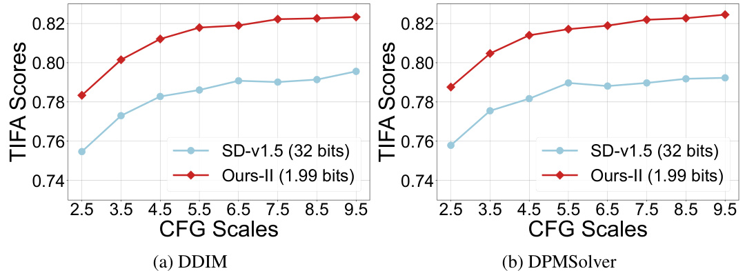
🔼 This figure compares the performance of the original Stable Diffusion v1.5 (32 bits) and the proposed BitsFusion (1.99 bits) method using different sampling schedulers (DDIM and DPMSolver). The x-axis represents the classifier-free guidance (CFG) scales, and the y-axis shows the TIFA scores. This figure demonstrates that BitsFusion consistently outperforms the original model across various CFG scales and sampling methods.
read the caption
Figure 16: TIFA scores comparisons between SD-v1.5 and BitsFusion, with different schedulers. Left: TIFA scores measured with DDIM [78] scheduler. Right: TIFA score measured with DPMSolver [55] scheduler.
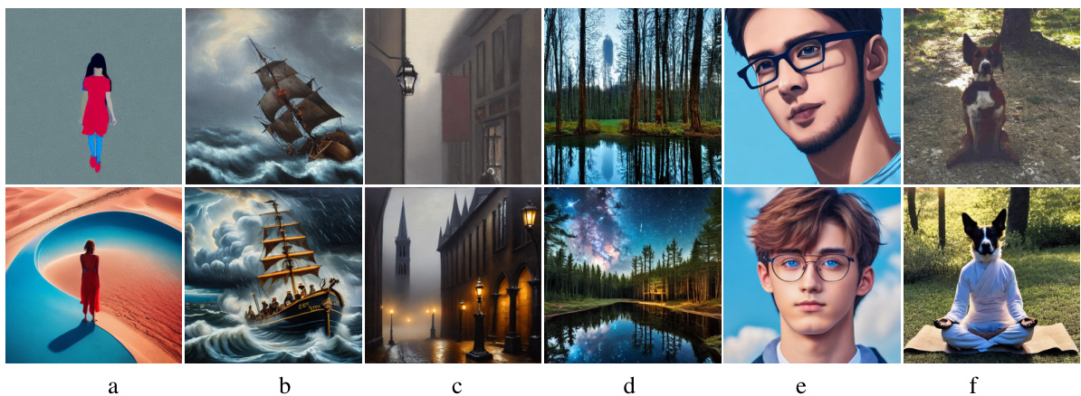
🔼 This figure shows a comparison of images generated using the full-precision Stable Diffusion v1.5 model and the BitsFusion model with 1.99-bit weight quantization. The top row displays images from the original Stable Diffusion, while the bottom row shows images generated by the quantized BitsFusion model. The images demonstrate that the quantized model achieves comparable image quality while significantly reducing model size (7.9x smaller). All images were generated using the same settings (PNDM sampler, 50 sampling steps, random seed 1024), differing only in the model used. Specific prompts used for each image are listed in Appendix M.
read the caption
Figure 1: Top: Images generated from full-precision Stable Diffusion v1.5. Bottom: Images generated from BitsFusion, where the weights of UNet are quantized into 1.99 bits, achieving 7.9× smaller storage than the one from Stable Diffusion v1.5. All the images are synthesized under the setting of using PNDM sampler [49] with 50 sampling steps and random seed as 1024. Prompts and more generations are provided in App. M.
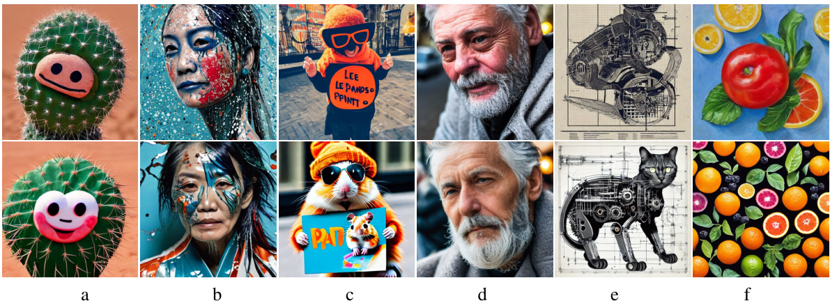
🔼 This figure shows a comparison of images generated by the full-precision Stable Diffusion v1.5 model and the BitsFusion model (with UNet weights quantized to 1.99 bits). The top row displays images from Stable Diffusion, and the bottom row displays images from BitsFusion. The images illustrate that BitsFusion achieves significantly reduced storage size (7.9 times smaller) while maintaining comparable image quality. All images were generated using the same settings (PNDM sampler, 50 sampling steps, random seed 1024). Prompts for image generation are detailed in Appendix M.
read the caption
Figure 1: Top: Images generated from full-precision Stable Diffusion v1.5. Bottom: Images generated from BitsFusion, where the weights of UNet are quantized into 1.99 bits, achieving 7.9× smaller storage than the one from Stable Diffusion v1.5. All the images are synthesized under the setting of using PNDM sampler [49] with 50 sampling steps and random seed as 1024. Prompts and more generations are provided in App. M.
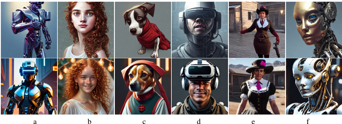
🔼 This figure showcases the image generation capabilities of both the original Stable Diffusion v1.5 model and the quantized BitsFusion model. The top row displays images created using the full-precision Stable Diffusion v1.5, demonstrating its baseline image quality. The bottom row presents images generated by BitsFusion, where the UNet’s weights have been quantized to 1.99 bits. Despite the significant reduction in model size (7.9 times smaller), BitsFusion maintains impressive image quality, comparable to the original Stable Diffusion v1.5. The generation parameters (sampler, steps, seed) were kept consistent for a fair comparison.
read the caption
Figure 1: Top: Images generated from full-precision Stable Diffusion v1.5. Bottom: Images generated from BitsFusion, where the weights of UNet are quantized into 1.99 bits, achieving 7.9× smaller storage than the one from Stable Diffusion v1.5. All the images are synthesized under the setting of using PNDM sampler [49] with 50 sampling steps and random seed as 1024. Prompts and more generations are provided in App. M.

🔼 This figure shows a comparison of images generated by the original Stable Diffusion model (top row) and the proposed BitsFusion model (bottom row). The BitsFusion model uses 1.99-bit weight quantization, significantly reducing the model size while maintaining comparable image quality. All images were generated using the same settings (PNDM sampler, 50 sampling steps, random seed 1024) for a fair comparison. The prompts used to generate these images can be found in Appendix M.
read the caption
Figure 1: Top: Images generated from full-precision Stable Diffusion v1.5. Bottom: Images generated from BitsFusion, where the weights of UNet are quantized into 1.99 bits, achieving 7.9× smaller storage than the one from Stable Diffusion v1.5. All the images are synthesized under the setting of using PNDM sampler [49] with 50 sampling steps and random seed as 1024. Prompts and more generations are provided in App. M.
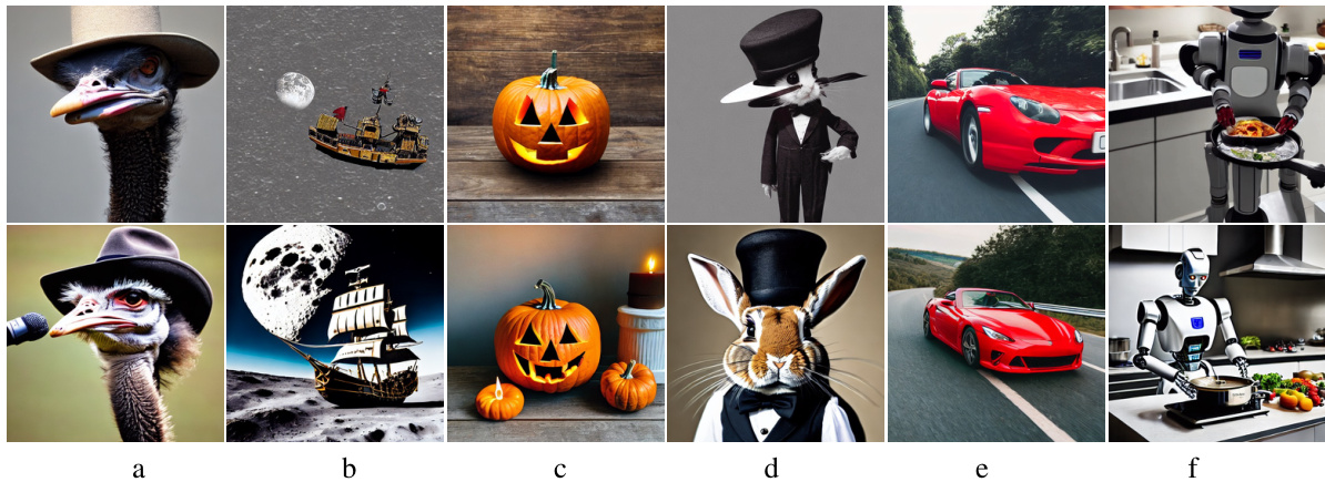
🔼 This figure shows a comparison of images generated by the full-precision Stable Diffusion v1.5 model and the BitsFusion model (with UNet weights quantized to 1.99 bits). The top row displays images generated using the full-precision model, while the bottom row shows images generated using the quantized BitsFusion model. The visual similarity demonstrates that the quantized model maintains high image quality despite its significantly reduced size (7.9x smaller). All images were created using the same parameters: PNDM sampler [49], 50 sampling steps, and a random seed of 1024. Specific prompts and additional generated images can be found in Appendix M.
read the caption
Figure 1: Top: Images generated from full-precision Stable Diffusion v1.5. Bottom: Images generated from BitsFusion, where the weights of UNet are quantized into 1.99 bits, achieving 7.9× smaller storage than the one from Stable Diffusion v1.5. All the images are synthesized under the setting of using PNDM sampler [49] with 50 sampling steps and random seed as 1024. Prompts and more generations are provided in App. M.

🔼 This figure shows a comparison of images generated using the full-precision Stable Diffusion v1.5 model and the BitsFusion model. The top row displays images generated by the original model, while the bottom row shows images generated by the quantized BitsFusion model. Each column represents a different image generated from a specific text prompt. The prompts are provided in the caption, and they vary in subject, style, and level of detail.
read the caption
Figure 17: Top: Images generated from full-precision Stable Diffusion v1.5. Bottom: Images generated from BitsFusion. Prompts from left to right are: a: A person standing on the desert, desert waves, gossip illustration, half red, half blue, abstract image of sand, clear style, trendy illustration, outdoor, top view, clear style, precision art, ultra high definition image; b: A detailed oil painting of an old sea captain, steering his ship through a storm. Saltwater is splashing against his weathered face, determination in his eyes. Twirling malevolent clouds are seen above and stern waves threaten to submerge the ship while seagulls dive and twirl through the chaotic landscape. Thunder and lights embark in the distance, illuminating the scene with an eerie green glow.; c: A solitary figure shrouded in mists peers up from the cobble stone street at the imposing and dark gothic buildings surrounding it. an old-fashioned lamp shines nearby. oil painting.; d: A deep forest clearing with a mirrored pond reflecting a galaxy-filled night sky; e: a handsome 24 years old boy in the middle with sky color background wearing eye glasses, it's super detailed with anime style, it's a portrait with delicated eyes and nice looking face; f: A dog that has been meditating all the time.

🔼 This figure shows a comparison of images generated by the full-precision Stable Diffusion v1.5 model and the BitsFusion model with 1.99-bit weight quantization. The top row displays images from the full-precision model, while the bottom row shows images from the quantized model. The images demonstrate that BitsFusion achieves comparable image quality with a significantly reduced model size (7.9 times smaller). The generation parameters (sampler, steps, seed) are kept consistent for both models.
read the caption
Figure 1: Top: Images generated from full-precision Stable Diffusion v1.5. Bottom: Images generated from BitsFusion, where the weights of UNet are quantized into 1.99 bits, achieving 7.9× smaller storage than the one from Stable Diffusion v1.5. All the images are synthesized under the setting of using PNDM sampler [49] with 50 sampling steps and random seed as 1024. Prompts and more generations are provided in App. M.
More on tables

🔼 This table presents the Pearson correlation coefficients between quantization errors obtained when quantizing individual layers to different bit-widths (1, 2, and 3 bits). Each cell shows the correlation for a single metric (MSE, PSNR, LPIPS, or CLIP score) between two different bit-widths. For instance, the value 0.929 in the first row and first column indicates a strong positive correlation (0.929) between the MSE obtained using 1-bit quantization and the MSE obtained using 2-bit quantization. This suggests that layers with high MSE in 1-bit quantization are likely to also have high MSE in 2-bit quantization. The table helps to understand the relationship between quantization errors across different bit-widths for each metric.
read the caption
Table 2: Pearson correlation (absolute value) of quantization error between different bit pairs (e.g., 1 vs. 2 denotes the correlation between the two bit widths) for a single metric when quantizing individual layers to 1, 2, and 3 bits.
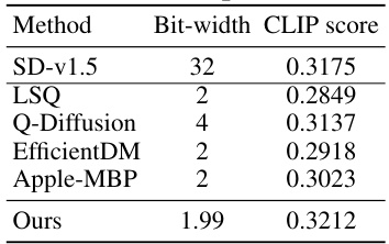
🔼 This table compares the performance of BitsFusion (the proposed method) against other existing weight quantization methods for diffusion models. The methods are compared based on their bit-width and the CLIP score achieved on a set of 1000 PartiPrompts. The CLIP score measures the alignment between generated images and their text descriptions, indicating the overall quality of the generated images.
read the caption
Table 3: Comparison with existing quantization methods, including LSQ [11], Q-Diffusion [38], EfficientDM [17], and Apple-MBP [62]. The CLIP score is measured on 1K PartiPrompts.

🔼 This table presents an ablation study, analyzing the impact of different techniques incorporated into the BitsFusion model on its performance. The baseline is a simple 2-bit quantization (LSQ). Subsequent rows add components of the BitsFusion method one at a time, showing how each contributes to the overall CLIP score. The results are evaluated across various CFG (Classifier-Free Guidance) scales to demonstrate robustness. The final row shows the overall improvement achieved by BitsFusion.
read the caption
Table 4: Analysis of our proposed methods measured under various CFG scales, i.e., 3.5, 5.5, 7.5, and 9.5. We use LSQ [11] as the basic QAT method, which involves the training of weights and scaling factors of a uniformly 2-bit quantized UNet. Then, we gradually introduce each proposed technique to evaluate their effectiveness. CLIP scores are measured on 1K PartiPrompts.

🔼 This table presents the results of an ablation study on the parameter size factor (η) used in the mixed-precision quantization strategy. Different values of η were tested (0, 0.1, 0.2, 0.3, 0.4, 0.5), and the corresponding CLIP scores are shown. The experiment aimed to determine the optimal value of η that balances model size reduction with maintaining good image generation quality.
read the caption
Table 5: Analysis of η in the mixed-precision strategy.

🔼 This table presents an ablation study evaluating the impact of different techniques incorporated into the BitsFusion model. It starts with a baseline method (LSQ) and sequentially adds components like balanced integer initialization, alternating optimization, mixed precision with caching, feature distillation, and time-step aware sampling. The results, measured by CLIP score on 1k PartiPrompts, show the performance improvement at each step, demonstrating the effectiveness of the proposed techniques in improving the quantization performance of the UNet in Stable Diffusion. The CFG (classifier-free guidance) scale is varied to show the model’s robustness across different guidance levels.
read the caption
Table 4: Analysis of our proposed methods measured under various CFG scales, i.e., 3.5, 5.5, 7.5, and 9.5. We use LSQ [11] as the basic QAT method, which involves the training of weights and scaling factors of a uniformly 2-bit quantized UNet. Then, we gradually introduce each proposed technique to evaluate their effectiveness. CLIP scores are measured on 1K PartiPrompts.
Full paper#


