TL;DR#
Existing graph foundation models struggle with generalizability and negative transfer across diverse tasks and domains. This is primarily due to challenges in defining transferable patterns on graphs, unlike images and text. Previous attempts focused on graphon theory or subgraph structures, but these are often limited in applicability or computationally intensive.
The paper proposes GFT, a novel graph foundation model that leverages computation trees derived from message-passing processes as transferable tokens. This approach demonstrates effectiveness by improving model generalization and reducing negative transfer. The effectiveness is shown via theoretical analysis and extensive experiments across diverse datasets and graph learning tasks. The model’s success shows the potential of computation trees as a foundational vocabulary for GFMs.
Key Takeaways#
Why does it matter?#
This paper is crucial for researchers in graph neural networks and machine learning. It introduces a novel approach to building graph foundation models (GFMs), addressing the limitations of existing methods. The concept of transferable computation trees as tokens is highly innovative and opens new avenues for improving model generalization and reducing negative transfer. This work is timely given the increasing importance of GFMs and its solutions are broadly applicable across various graph learning tasks.
Visual Insights#
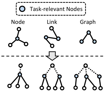
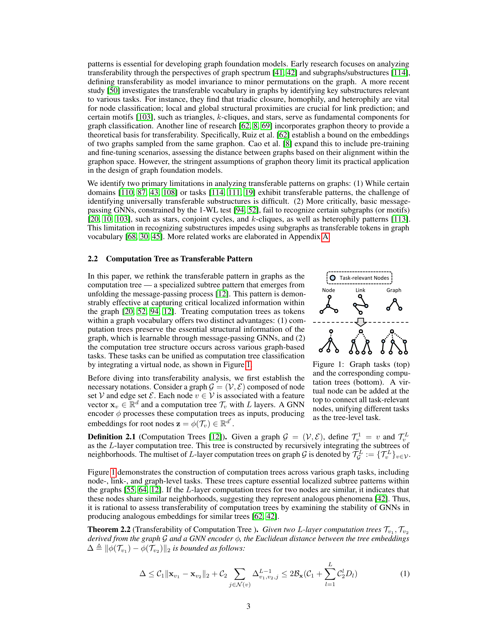
🔼 This figure illustrates how computation trees can represent various graph tasks. The top row shows examples of node-level, link-level, and graph-level tasks. The bottom row shows the corresponding computation trees derived from the message-passing process of a graph neural network. A key aspect is the addition of a virtual node to connect task-relevant nodes, making it possible to unify different graph tasks into a single ’tree-level’ task.
read the caption
Figure 1: Graph tasks (top) and the corresponding computation trees (bottom). A virtual node can be added at the top to connect all task-relevant nodes, unifying different tasks as the tree-level task.

🔼 This table presents the results of transfer learning experiments conducted on both homophilic and heterophilic graphs. It demonstrates a correlation between the computation tree similarity between source and target graphs and the transfer learning performance. Higher tree similarity between graphs generally leads to better transfer learning accuracy, while the impact of motif similarity is less significant. The table is divided into two parts, one for homophilic graphs (airport networks) and one for heterophilic graphs (WebKB networks), with each part showing results for various combinations of source and target graphs.
read the caption
Table 1: Transfer learning performance on homophily (above) and heterophily (below) graphs. For any target graph, source graphs with higher tree similarity lead to improved accuracy, highlighted with Blue. Conversely, the influence of motif similarity is marginal, marked by LightBlue.
In-depth insights#
GFT: Graph Foundation#
The heading “GFT: Graph Foundation” suggests a research paper focusing on a novel graph foundation model. A graph foundation model, analogous to large language models (LLMs) or large vision models (LVMs), aims to be a general-purpose model pre-trained on vast amounts of graph data. GFT likely leverages a transferable tree vocabulary, meaning that the model represents graph information using computation trees, enabling knowledge transfer between various graph-related tasks and domains. This approach tackles the challenge of defining transferable patterns for graphs, which differs significantly from images or text. The “transferable” aspect highlights the model’s ability to generalize across different graph types and tasks, improving performance and reducing negative transfer, unlike previous pre-trained graph neural network (GNN) models. The name “Graph Foundation” emphasizes its role as a foundational model, potentially serving as a basis for numerous downstream graph-based applications.
Transferable Tree#
The concept of “Transferable Tree” in a research paper likely revolves around representing and utilizing tree-like structures to capture transferable knowledge across diverse graph-based tasks. This approach likely addresses the limitations of existing methods by focusing on computation trees, which are derived from the message-passing process in graph neural networks (GNNs). The key idea is that these computation trees encode transferable patterns shared across various tasks and domains, forming a universal vocabulary for graph learning. Treating these trees as tokens in the vocabulary improves model generalization, reduces negative transfer, and increases efficiency by integrating tree extraction and encoding into the GNN message-passing process. The theoretical analysis and experimental validation demonstrate the effectiveness of this approach. The research likely explores different aspects like tree reconstruction, tree classification, vocabulary quantization, and the impact of computation tree similarity on transfer learning performance. Generalization and scalability of the proposed method are likely also considered, comparing it to traditional subgraph-based and LLMs-based approaches. Ultimately, “Transferable Tree” represents an innovative approach towards building robust and generalizable graph foundation models.
Computation Tree#
The concept of a ‘Computation Tree’ in the context of graph neural networks (GNNs) offers a novel perspective on transferable patterns within graph data. Instead of relying on subgraphs or graph spectra, which may not fully capture relevant information or be efficiently extractable, computation trees leverage the inherent structure of the message-passing process in GNNs. Each node’s computation tree represents the flow of information during message passing, effectively encapsulating localized patterns critical for various graph learning tasks. This approach offers efficiency advantages as computation tree extraction is integrated within the GNN computation itself, unlike explicit subgraph extraction, which is computationally more expensive. The use of computation trees as tokens in a transferable vocabulary allows for a unified representation across different graph tasks, improving model generalization and transferability. The effectiveness hinges on the ability of GNNs to learn and represent computation tree patterns, which are then quantized to form a discrete vocabulary for efficient representation and subsequent use in classification tasks. This theoretically grounded approach promises to advance the field of graph foundation models, significantly improving model performance in diverse applications.
GFT: Model Transfer#
The heading “GFT: Model Transfer” suggests a section dedicated to exploring the model’s ability to generalize knowledge learned from one task or domain to another. This likely involves a discussion of transfer learning techniques implemented in GFT, possibly including pre-training strategies on large, diverse datasets to establish a strong foundational knowledge base. The core of this section would focus on demonstrating the effectiveness of GFT’s transfer capabilities across various tasks (e.g., node, link, graph classification) and domains. Quantitative results showing performance improvements on target tasks after transfer learning, compared to models trained from scratch, would be crucial. Furthermore, the section would likely delve into the mechanisms underlying GFT’s transferability, analyzing the role of the ’transferable Tree vocabulary’ in facilitating knowledge transfer. A qualitative discussion of how GFT handles potential issues like negative transfer—where pre-training hinders performance on the target task—would also be expected. Finally, the analysis may include comparisons with other state-of-the-art transfer learning approaches for graph neural networks, highlighting GFT’s unique strengths and limitations in this area.
Future of GFT#
The future of GFT (Graph Foundation Model with Transferable Tree Vocabulary) looks promising, given its demonstrated effectiveness in cross-domain and cross-task graph learning. Further research could focus on enhancing its scalability and efficiency for even larger graphs, perhaps by exploring more sophisticated tree encoding and aggregation techniques. Integrating GFT with other foundation models, such as large language models (LLMs) or large vision models (LVMs), would open exciting new avenues for multimodal graph analysis and knowledge discovery. Investigating its application in diverse domains beyond those explored in the paper, such as drug discovery, financial modeling and climate change analysis, should reveal additional valuable insights and practical applications. Addressing potential limitations related to the expressiveness of message-passing GNNs and the choice of computation tree representation are crucial for robust generalization. Finally, further theoretical analysis to more precisely define the transferability of computation trees and their relationship to various graph properties would strengthen the foundation of GFT and guide future developments.
More visual insights#
More on figures

🔼 This figure shows three synthetic graphs (G1, G2, and G3) constructed from two basic blocks. The number of blocks is varied to demonstrate how the size of the graphs can be increased. These graphs are used in the experiments to study the transferability of computation trees, showing how the similarity of tree structures affects the ability of a model to generalize to new tasks.
read the caption
Figure 2: Synthetic graphs composed of two basic blocks. More blocks can scale up the graph sizes.

🔼 This figure illustrates the two-stage training process of the GFT model. In the pre-training stage (a), a graph database is used to generate computation trees which are encoded into a tree vocabulary via a tree reconstruction task. This involves reconstructing features of the root node, the connectivity among nodes, and the semantics of the trees. An orthogonal regularizer is applied to improve the quality of the tree vocabulary. In the fine-tuning stage (b), the pre-trained tree vocabulary is used to unify graph-related tasks (node, link, and graph-level) into a computation tree classification task. This involves querying the fixed tree vocabulary, classifying computation trees, and using both a prototype classifier and a linear classifier to generate predictions. The process adapts the general knowledge encoded in the tree vocabulary to specific tasks.
read the caption
Figure 4: During pre-training, GFT encodes general knowledge from a graph database into a tree vocabulary through tree reconstruction. In fine-tuning, the learned tree vocabulary is applied to unify graph-related tasks as tree classification, adapting the general knowledge to specific tasks.
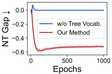
🔼 The figure shows the negative transfer gap (NT gap) on the Cora dataset for node classification. The NT gap is calculated as R(S,T) - R(0,T), where R(S,T) is the risk on task T with pre-training on task S and R(0,T) is the risk without pre-training. The plot compares the NT gap for two approaches: one without a tree vocabulary and the other using the authors’ proposed method (GFT). The results illustrate that employing the learned tree vocabulary to align the tree reconstruction task (pre-training) and tree classification task (fine-tuning) significantly reduces negative transfer. The y-axis represents the NT gap and the x-axis represents the number of training epochs.
read the caption
Figure 5: Negative transfer gap on Cora in node classification.
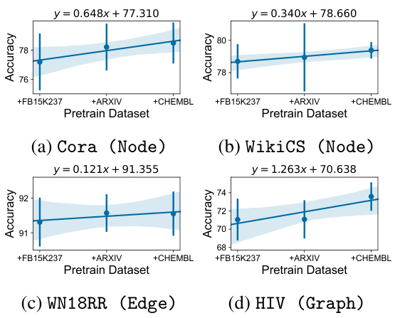
🔼 This figure shows the impact of using different combinations of pre-training datasets on the performance of GFT across four different graph datasets (Cora, WikiCS, WN18RR, and HIV). Each subplot represents a different dataset and task (node classification, node classification, link prediction, and graph classification, respectively). The x-axis shows the combination of pre-training datasets used (FB15k237, Arxiv, and Chembl), and the y-axis shows the accuracy achieved by GFT. The lines represent the trend of accuracy with an increasing number of pre-training datasets used. The shaded area indicates the standard deviation of the accuracy over multiple runs. This figure demonstrates that GFT consistently achieves better performance as more pre-training datasets are used, illustrating the effectiveness of the model in learning transferable patterns across diverse graphs.
read the caption
Figure 7: GFT consistently improves model performance with more pre-training datasets.

🔼 This figure compares the efficiency of using computation trees versus subgraphs for GFT model training. It shows memory usage and training time per epoch across different batch sizes. The results demonstrate that the computation tree approach is significantly more memory-efficient and scalable, as subgraph-based methods run out of memory at larger batch sizes.
read the caption
Figure 8: The efficiency analysis between computation trees and subgraphs. Our GFT is based on the computation trees and we further replace the computation trees with subgraphs called GFT-Subgraph. We compare their memory usage (a) and time consumption (b) during pretraining. With the increase of batch sizes, Subgraph-based GFT encounters out-of-memory, yet computation tree-based GFT can still fit in the GPU.
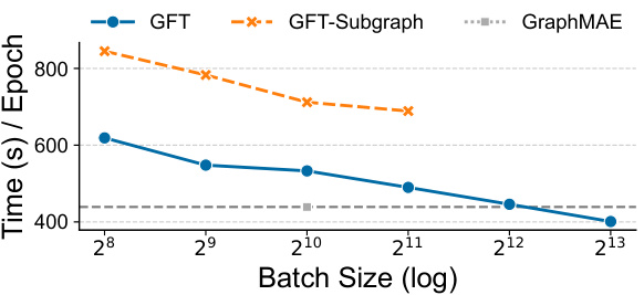
🔼 This figure compares the efficiency of using computation trees versus subgraphs in the GFT model. The top graph shows memory usage, and the bottom shows the time taken per epoch, both plotted against increasing batch size (log scale). The results indicate that using computation trees is significantly more memory-efficient and allows for much larger batch sizes before running into out-of-memory errors, compared to using subgraphs. This highlights the efficiency advantage of GFT’s approach.
read the caption
Figure 8: The efficiency analysis between computation trees and subgraphs. Our GFT is based on the computation trees and we further replace the computation trees with subgraphs called GFT-Subgraph. We compare their memory usage (a) and time consumption (b) during pretraining. With the increase of batch sizes, Subgraph-based GFT encounters out-of-memory, yet computation tree-based GFT can still fit in the GPU.

🔼 This figure illustrates the two-stage training process of the GFT model. The pre-training phase uses a tree reconstruction task to learn a general tree vocabulary from a diverse graph database. This vocabulary captures fundamental patterns common to different graph tasks. In the fine-tuning stage, this vocabulary is utilized to unify various graph tasks (node, link, and graph level) as a single tree classification task, thus improving model generalization and reducing negative transfer.
read the caption
Figure 4: During pre-training, GFT encodes general knowledge from a graph database into a tree vocabulary through tree reconstruction. In fine-tuning, the learned tree vocabulary is applied to unify graph-related tasks as tree classification, adapting the general knowledge to specific tasks.

🔼 This figure illustrates how different graph tasks (node, link, and graph classification) can be represented as computation trees. A computation tree is a specialized subtree pattern derived from unfolding the message-passing process in a graph neural network. By adding a virtual node at the top of the computation tree, all the task-relevant nodes are connected, unifying the different graph tasks as a single tree-level classification task. This shows the basic idea behind using computation trees as transferable patterns across various graph tasks.
read the caption
Figure 1: Graph tasks (top) and the corresponding computation trees (bottom). A virtual node can be added at the top to connect all task-relevant nodes, unifying different tasks as the tree-level task.

🔼 This figure shows the relationship between computation tree similarity and transfer learning performance on synthetic graphs. Three distinct graphs (G1, G2, G3) were constructed. G1 and G2 share similar motifs but have different computation tree distributions. G1 and G3 have dissimilar motifs but similar computation tree distributions. The x-axis represents the number of blocks used to construct the synthetic graphs, representing the scale of the graph. The y-axis on the leftmost subplot shows the transferability, measured using the inverse of the Central Moment Discrepancy (CMD). The y-axis on the middle subplot represents the computation tree similarity (Tree Sim.) measured using the Weisfeiler-Lehman subtree kernel. The y-axis on the rightmost subplot displays the motif similarity (Motif Sim.) measured using the graphlet sampling kernel. The results indicate that higher computation tree similarity is strongly correlated with improved transfer learning performance, while motif similarity shows less correlation.
read the caption
Figure 3: Transfer performance on synthetic graphs with G1 as the target graph. Higher tree similarity correlates with enhanced transferability.

🔼 This figure shows the results of transfer learning experiments on synthetic graphs. Three different graphs (G1, G2, and G3) were used, with G1 being the target graph. The graphs were designed to have varying levels of computation tree similarity and motif similarity. The x-axis represents the number of blocks in the graph, which is a measure of the graph’s size. The y-axis represents transferability, which is measured using the inverse of the Central Moment Discrepancy (CMD). The figure demonstrates that higher tree similarity between the source and target graphs correlates strongly with improved transferability, while the impact of motif similarity is less pronounced. This supports the paper’s central argument that computation trees are more effective transferable patterns than motifs for graph learning.
read the caption
Figure 3: Transfer performance on synthetic graphs with G1 as the target graph. Higher tree similarity correlates with enhanced transferability.
More on tables

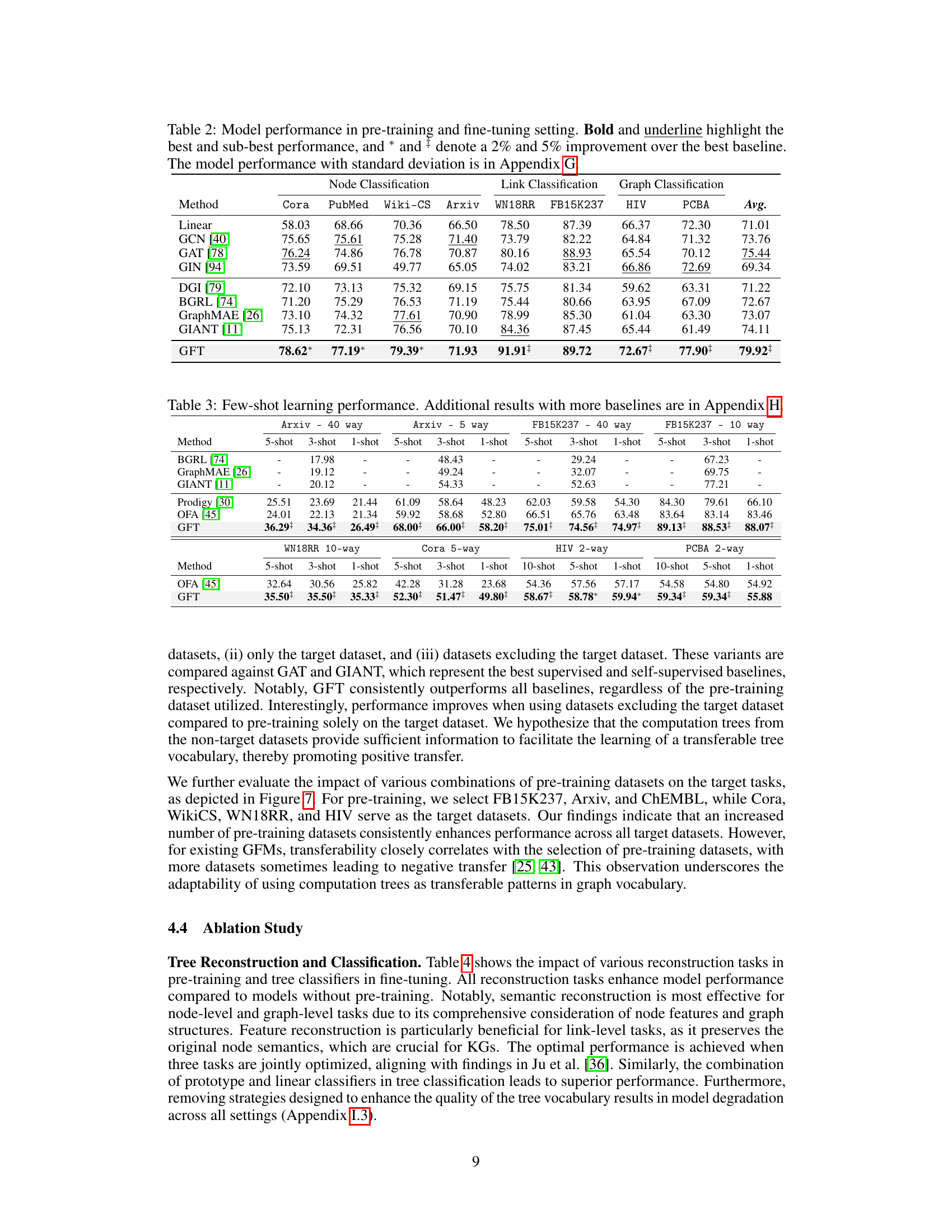
🔼 This table presents the performance of various models (including the proposed GFT model) on node, link, and graph classification tasks. The results are split based on the dataset and the task. The best and second-best performances for each task and dataset are highlighted, indicating the performance gain of the GFT model compared to existing methods. Detailed results with standard deviations are available in Appendix G.
read the caption
Table 2: Model performance in pre-training and fine-tuning setting. Bold and underline highlight the best and sub-best performance, and * and * denote a 2% and 5% improvement over the best baseline. The model performance with standard deviation is in Appendix G.

🔼 This table shows the few-shot learning performance of the GFT model compared to other self-supervised methods and graph foundation models. The results are presented for various datasets and different numbers of shots (training instances per class). The table highlights GFT’s superior performance, especially when training instances are extremely limited.
read the caption
Table 3: Few-shot learning performance. Additional results with more baselines are in Appendix H.

🔼 This table presents the ablation study results on the tree reconstruction tasks in pre-training and tree classifiers in fine-tuning. It shows the impact of various reconstruction tasks (reconstructing features of the root node, connectivity among nodes, and overall semantics of computation trees) in pre-training on the model performance across node-level, link-level, and graph-level tasks. It also shows the comparison results with different tree classifiers (prototype classifier and linear classifier).
read the caption
Table 4: Ablation on tree reconstruction (above) and tree classification (bottom).
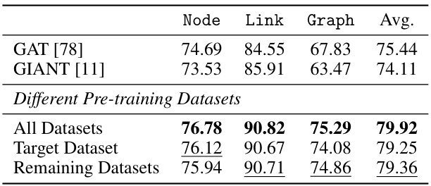
🔼 This table presents the performance of various models in node, link, and graph classification tasks, comparing the GFT model with baselines such as GCN, GAT, GIN, DGI, BGRL, GraphMAE, and GIANT. The results are shown for pre-training and fine-tuning settings, indicating the average performance across multiple datasets with standard deviations detailed in Appendix G. The best and second-best performances are highlighted, with additional notes on performances that exceed baselines by 2% and 5%.
read the caption
Table 2: Model performance in pre-training and fine-tuning setting. Bold and underline highlight the best and sub-best performance, and * and * denote a 2% and 5% improvement over the best baseline. The model performance with standard deviation is in Appendix G.
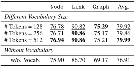
🔼 This table presents the results of an ablation study evaluating the effect of using different sizes of tree vocabulary and a setting without a tree vocabulary in the GFT model. It compares the average performance across node, link, and graph classification tasks for various vocabulary sizes, showing the impact of the tree vocabulary on model performance. The results demonstrate that using the tree vocabulary enhances model generalization and improves performance across various tasks.
read the caption
Table 6: The impact of tree vocabulary.

🔼 This table compares the performance of using computation trees versus subgraphs as transferable patterns in the GFT model. It shows accuracy results for node, link, and graph classification tasks across four models: GAT, GraphMAE, GFT with subgraphs (GFT - Subgraph), and GFT with computation trees (GFT - Tree). The results highlight the superior performance of using computation trees over subgraphs for various graph tasks.
read the caption
Table 7: The comparison between computation trees and subgraphs.

🔼 This table compares the number of parameters across various graph foundation models, including Prodigy, OFA, UniGraph, and the proposed GFT model. It highlights the relative model complexity and efficiency, demonstrating that GFT achieves comparable performance with significantly fewer parameters than some of the other models.
read the caption
Table 8: Comparison of number of parameters across different models

🔼 This table presents the results of transfer learning experiments conducted on both homophily and heterophily graph datasets. It shows the relationship between computation tree similarity (a measure of how similar the computation trees of two graphs are), motif similarity (a measure of how similar the graph motifs of two graphs are), and transfer learning performance (accuracy). The table highlights that higher computation tree similarity correlates with better transfer learning accuracy, while motif similarity has a less significant effect.
read the caption
Table 1: Transfer learning performance on homophily (above) and heterophily (below) graphs. For any target graph, source graphs with higher tree similarity lead to improved accuracy, highlighted with Blue. Conversely, the influence of motif similarity is marginal, marked by LightBlue.

🔼 This table presents the statistics of nine graph datasets used in the experiments, including the domain, task type, number of graphs, average number of nodes and edges, and number of classes. The datasets represent various types of graphs, including citation networks, web link networks, knowledge graphs, and molecular graphs, covering node-level, link-level, and graph-level tasks.
read the caption
Table 10: Dataset statistics [45].

🔼 This table lists the hyperparameters used for fine-tuning the GFT model across different datasets. It includes learning rate, number of epochs, early stopping criteria, batch size, number of instances per class used for creating prototypes, temperature parameters for both prototype and linear classifiers, and weights for the loss functions of these classifiers.
read the caption
Table 11: Hyper-parameters in fine-tuning.

🔼 This table shows the performance comparison of various models on different tasks (node, link, and graph classification) and datasets. The models are compared under two training schemes: pre-training and fine-tuning. The best performing models are highlighted and improvement over the best baseline is also specified.
read the caption
Table 2: Model performance in pre-training and fine-tuning setting. Bold and underline highlight the best and sub-best performance, and * and * denote a 2% and 5% improvement over the best baseline. The model performance with standard deviation is in Appendix G.

🔼 This table presents the few-shot learning performance of the GFT model compared to several baselines, including self-supervised methods and other graph foundation models. It shows the performance across different datasets and different numbers of shots (training samples per class) for node and link classification tasks. The results demonstrate the effectiveness of GFT in few-shot learning scenarios.
read the caption
Table 3: Few-shot learning performance. Additional results with more baselines are in Appendix H.

🔼 This table presents the average performance of different models across various graph datasets and tasks in both pre-training and fine-tuning settings. The models include supervised and self-supervised GNNs, as well as graph foundation models. The table highlights the superior performance of the GFT model, with significant improvements over the best baseline in most cases, indicating its ability to transfer learning effectively across different tasks and domains.
read the caption
Table 2: Model performance in pre-training and fine-tuning setting. Bold and underline highlight the best and sub-best performance, and * and * denote a 2% and 5% improvement over the best baseline. The model performance with standard deviation is in Appendix G.

🔼 This table presents the few-shot learning performance of the GFT model compared to several baselines. Few-shot learning is a technique where the model is trained with a limited number of labeled examples per class. The table shows the performance across different tasks and datasets, and for various numbers of training examples per class (shots). The results demonstrate that GFT significantly outperforms the baselines even with limited training data, highlighting its effectiveness in few-shot learning scenarios.
read the caption
Table 3: Few-shot learning performance. Additional results with more baselines are in Appendix H.

🔼 This table presents the few-shot learning performance of the GFT model compared to several baselines (BGRL, GraphMAE, GIANT, Prodigy, OFA) across different datasets (Arxiv, FB15K237, Cora, HIV, PCBA) and various shot settings (1-shot, 3-shot, 5-shot) with different numbers of training instances per class (5, 10, 20, 30). The results showcase GFT’s superior performance in few-shot learning scenarios, emphasizing its ability to rapidly adapt to new tasks with limited labeled data.
read the caption
Table 3: Few-shot learning performance. Additional results with more baselines are in Appendix H.

🔼 This table presents the results of few-shot learning experiments, comparing the performance of GFT against various baselines across different datasets and settings. The results demonstrate the effectiveness of GFT, particularly in low-shot learning scenarios where training data is limited. The table showcases performance for different numbers of shots (e.g., 1-shot, 3-shot, 5-shot) and across various datasets (e.g., Arxiv, FB15K237, Cora, HIV, PCBA). Appendix H provides more detailed results with additional baselines.
read the caption
Table 3: Few-shot learning performance. Additional results with more baselines are in Appendix H.

🔼 This table presents the few-shot learning performance of the GFT model compared to other self-supervised methods and graph foundation models. The results show accuracy across various datasets (Arxiv, FB15K237, Cora, and HIV) with different numbers of shots (1, 3, 5, 10) and training instances per class (indicated by # train). It demonstrates GFT’s effectiveness with limited labeled data during the fine-tuning phase. Appendix H contains additional results.
read the caption
Table 3: Few-shot learning performance. Additional results with more baselines are in Appendix H.

🔼 This table presents the few-shot learning performance of the proposed model (GFT) and other existing models. Few-shot learning is a setting where models are trained on a limited number of examples for each class. The table shows the performance of different models across several datasets and varying numbers of training examples per class (shot). The results highlight the effectiveness of GFT in low-data scenarios.
read the caption
Table 3: Few-shot learning performance. Additional results with more baselines are in Appendix H.

🔼 This table presents the performance of various models on node classification, link classification, and graph classification tasks, comparing the performance of GFT with various baseline models. The results are presented as the average accuracy across multiple runs, with standard deviations reported in Appendix G. Bold and underlined values indicate the best and second-best performances, respectively, and asterisks indicate performance improvements (2% or 5%) over the best baseline. The table highlights the effectiveness of GFT’s cross-domain and cross-task transferability.
read the caption
Table 2: Model performance in pre-training and fine-tuning setting. Bold and underline highlight the best and sub-best performance, and * and * denote a 2% and 5% improvement over the best baseline. The model performance with standard deviation is in Appendix G.

🔼 This table shows the performance of different models (including the proposed GFT model) on various node, link, and graph classification tasks. The results are presented for several benchmark datasets, showing the average performance across multiple runs to account for randomness. The table indicates significant performance gains by GFT compared to other baselines (especially on link and graph classification tasks) highlighting the efficacy of the proposed transferable tree vocabulary.
read the caption
Table 2: Model performance in pre-training and fine-tuning setting. Bold and underline highlight the best and sub-best performance, and * and * denote a 2% and 5% improvement over the best baseline. The model performance with standard deviation is in Appendix G.

🔼 This table presents the performance of different models across various graph datasets and tasks, including node classification, link classification, and graph classification. The results are shown for both pre-training and fine-tuning settings. GFT demonstrates consistently better performance than the other models across a range of datasets, significantly outperforming the best baseline in several cases. The table highlights the effectiveness of the GFT model in leveraging computation trees as transferable patterns. Standard deviations for all results can be found in Appendix G.
read the caption
Table 2: Model performance in pre-training and fine-tuning setting. Bold and underline highlight the best and sub-best performance, and * and * denote a 2% and 5% improvement over the best baseline. The model performance with standard deviation is in Appendix G.

🔼 This table presents the performance of different models (including the proposed GFT model) on various graph-related tasks (Node, Link, and Graph classification). The results are obtained using both pre-training and fine-tuning procedures. The best and second-best performing models are highlighted. The table also indicates improvements of the GFT model compared to the best baselines. More detailed results, including standard deviations, can be found in Appendix G.
read the caption
Table 2: Model performance in pre-training and fine-tuning setting. Bold and underline highlight the best and sub-best performance, and * and * denote a 2% and 5% improvement over the best baseline. The model performance with standard deviation is in Appendix G.

🔼 This table presents the average performance of different models across various graph datasets for node, link, and graph classification tasks, comparing supervised and self-supervised models with the proposed GFT model. It highlights the superior performance of GFT compared to other state-of-the-art models. The results include standard deviations (available in Appendix G) providing a more complete understanding of the model’s performance.
read the caption
Table 2: Model performance in pre-training and fine-tuning setting. Bold and underline highlight the best and sub-best performance, and * and * denote a 2% and 5% improvement over the best baseline. The model performance with standard deviation is in Appendix G.
Full paper#
