↗ OpenReview ↗ NeurIPS Homepage ↗ Chat
TL;DR#
Denoising diffusion models (DDMs) are powerful generative AI tools, but their performance heavily relies on carefully chosen ‘discretization schedules.’ Finding these schedules usually involves manual trial-and-error, which is time-consuming and may not yield optimal results. This research addresses this significant issue.
The researchers propose a novel algorithm that automatically learns the optimal schedules by minimizing a newly defined ‘cost’ function. This cost function reflects the computational work needed to accurately simulate the model’s sampling process. Importantly, the algorithm is efficient, data-dependent, and doesn’t require parameter tuning. Experiments on various datasets show that it recovers previously known optimal schedules and achieves competitive results, highlighting its potential to improve the efficiency and quality of DDMs.
Key Takeaways#
Why does it matter?#
This paper is significant because it presents a novel algorithm for optimizing diffusion model sampling, a crucial aspect of generative AI. The algorithm is data-dependent, adaptive, and scalable, addressing a major limitation of existing methods that rely on manual tuning. This opens new avenues for research in improving the efficiency and quality of generative models and has implications for various applications. It also offers a new geometric interpretation that could influence the design and development of DDM samplers.
Visual Insights#

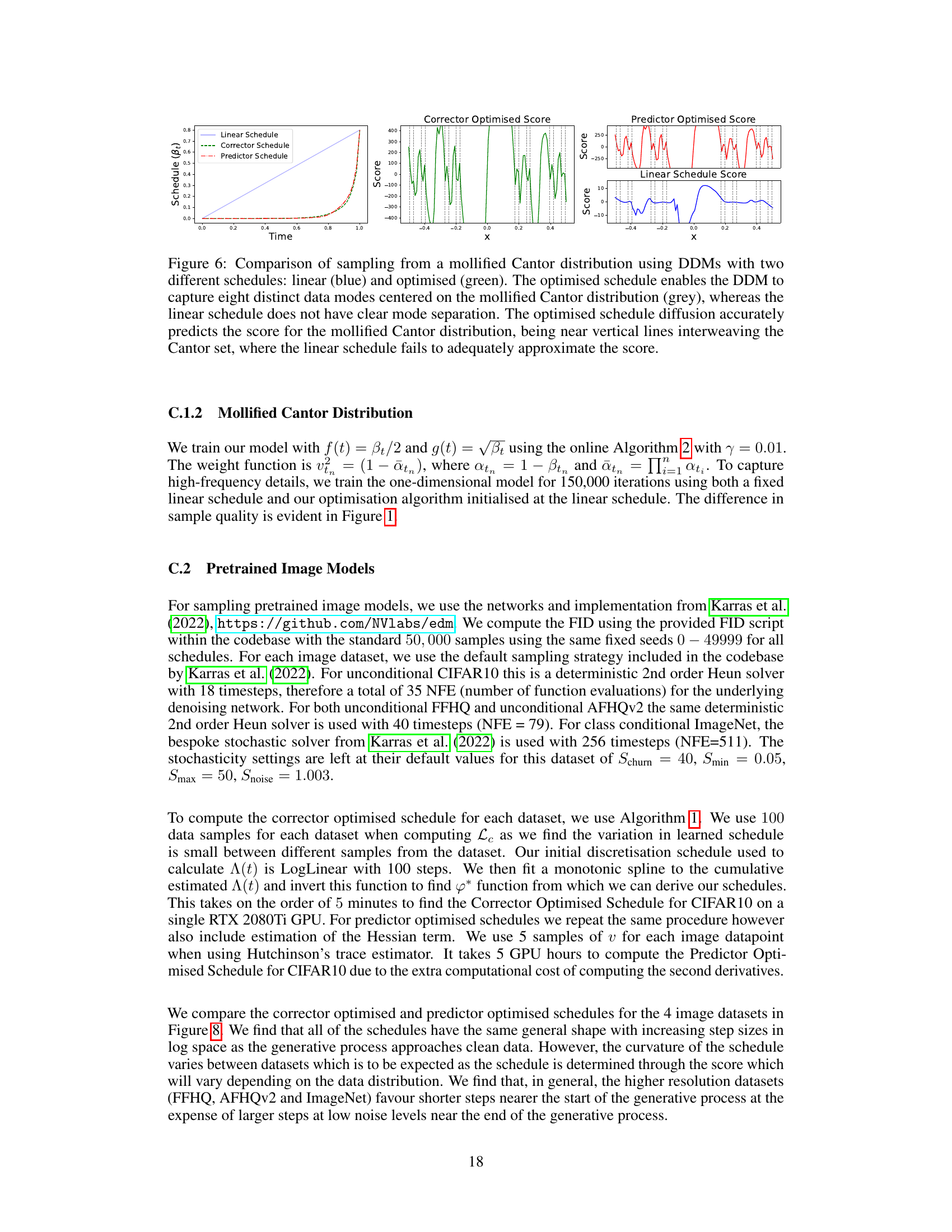
This figure compares density estimations of a mollified Cantor distribution generated using three different methods. The leftmost plot shows the actual density of the mollified Cantor distribution. The middle plot shows the density estimate generated by a Denoising Diffusion Model (DDM) using a linear schedule, which clearly fails to capture the eight modes of the distribution. The rightmost plot shows the density estimate generated by a DDM using an optimized schedule generated by the proposed Algorithm 1, which accurately captures the eight modes.

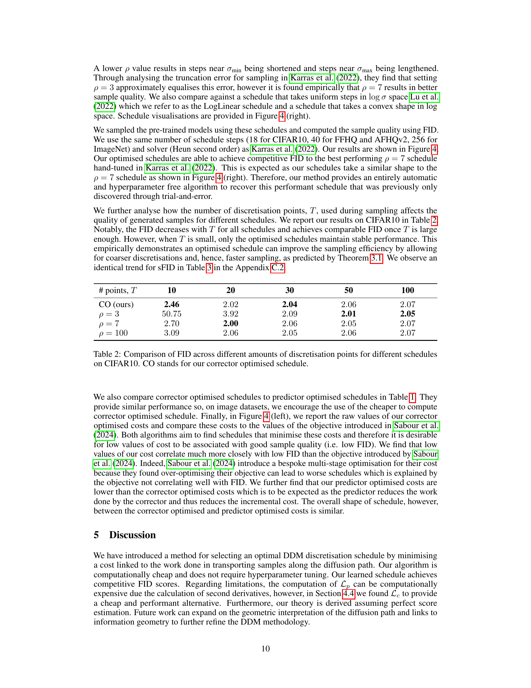
This table compares the Fréchet Inception Distance (FID) scores, a measure of sample quality, for different schedules used in sampling from pre-trained diffusion models on four image datasets: CIFAR-10, FFHQ, AFHQv2, and ImageNet. The schedules compared include various previously proposed methods (Eq (22) with ρ=3 and ρ=7, LogLinear, Convex), and the novel corrector and predictor-optimized schedules proposed in the paper. The best FID score for each dataset is highlighted in bold. Note that the ImageNet results only include the corrector-optimized schedule because the model lacks second-order differentiation, which is needed for the predictor-optimized schedule.
In-depth insights#
Score-Optimal DDM#
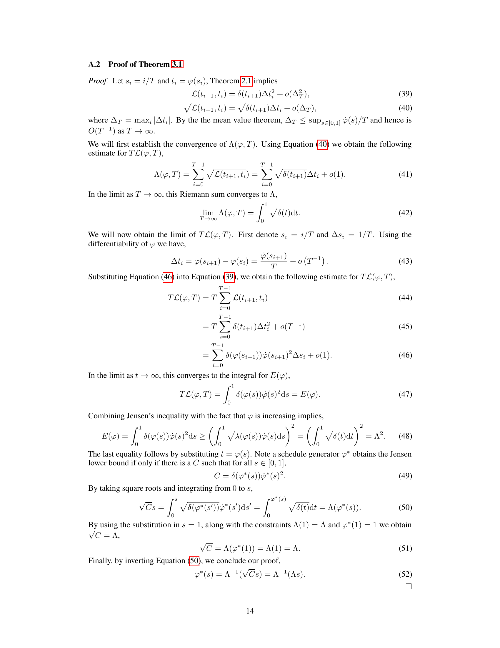
The concept of “Score-Optimal DDM” suggests a significant advancement in denoising diffusion models (DDMs). Optimizing the discretisation schedule is crucial for efficient and high-quality sample generation. This approach likely involves deriving a cost function that quantifies the computational effort of moving samples along the diffusion path, and then determining a schedule that minimizes this cost. This data-dependent adaptive approach would lead to significant improvements over existing, often manually tuned, methods. The key here is finding a balance between computational efficiency and the accuracy of the generated samples. Score matching plays a vital role; by incorporating estimated Stein scores, the algorithm adapts to the specific characteristics of the data distribution. The resulting algorithm would be highly scalable, suitable for both pre-trained and online model training.
Adaptive Schedule#
The concept of an ‘Adaptive Schedule’ in the context of a research paper likely refers to a dynamic adjustment of parameters within an algorithm or model over time. This contrasts with a static, pre-defined schedule where parameters remain constant. The adaptation could involve adjusting the learning rate, step size, or other hyperparameters based on the algorithm’s performance or feedback from the data. Key benefits of an adaptive schedule might include improved efficiency by optimizing for changing data characteristics or task demands, and enhanced robustness to noise and variations in data quality. The adaptive nature allows for self-regulation, enabling the model to learn optimal settings. A sophisticated adaptive schedule would likely incorporate mechanisms to monitor performance, detect changes, and trigger appropriate adjustments. Potential challenges in designing and evaluating an adaptive schedule might include computational overhead, complexity of implementation, and the difficulty of determining optimal adaptation strategies.
Cost of Correction#
The concept of ‘Cost of Correction’ in the context of diffusion models is crucial for understanding the efficiency of the sampling process. It essentially quantifies the computational effort required to steer samples generated by a predictor step back onto the desired diffusion path. The cost is directly related to the discrepancy between the distribution of predictor samples and the target distribution at a given time step. A low cost of correction indicates that the predictor is accurate and the corrective step is relatively easy, whereas a high cost implies significant deviation and substantial computational work to correct the trajectory. The paper leverages this cost function to devise an optimal discretisation schedule by minimising the cumulative cost across the entire diffusion process. This minimisation leads to computationally efficient and high-quality sample generation from complex data distributions. The cost function itself can be defined using metrics like the Stein divergence, making it sensitive to the specific dynamics and geometry of the data distribution.
Empirical Results#
An Empirical Results section would ideally present a thorough evaluation of the proposed score-optimal diffusion scheduling algorithm. This would involve comparing its performance against existing state-of-the-art methods across various datasets and metrics. Key metrics should include FID (Fréchet Inception Distance) and other relevant image quality measures to assess the generated samples’ visual fidelity. The analysis should go beyond simply reporting numerical results; it should include visualizations of the generated samples to demonstrate the algorithm’s effectiveness. Furthermore, a discussion on the computational efficiency of the proposed method compared to existing approaches is crucial. Finally, ablation studies demonstrating the individual contributions of different components of the algorithm (e.g., the predictor and corrector modules) are valuable in gaining a deeper understanding of the approach’s effectiveness and potential for future development. The use of rigorous statistical testing and error analysis should further enhance the reliability of the findings and strengthen the overall impact of the study.
Future Work#
Future work could explore several promising directions. Extending the theoretical framework to handle imperfect score estimation is crucial for real-world applications. This involves developing robust methods that account for score noise and uncertainty, potentially leveraging techniques from robust statistics or Bayesian inference. Investigating the geometric interpretation of the diffusion path, particularly its relationship to information geometry, could provide deeper insights into optimal schedule design and potentially lead to more efficient sampling strategies. Developing a more efficient algorithm for computing the predictor-optimized cost, which currently involves computationally expensive Hessian computations, is another important area. Exploring alternative predictor-corrector schemes or approximation techniques could significantly improve scalability. Finally, empirical evaluation on a wider range of datasets and model architectures is necessary to validate the generality and robustness of the proposed approach. This includes exploring high-dimensional datasets and investigating the effect of different model architectures on the performance of the score-optimal diffusion schedule.
More visual insights#
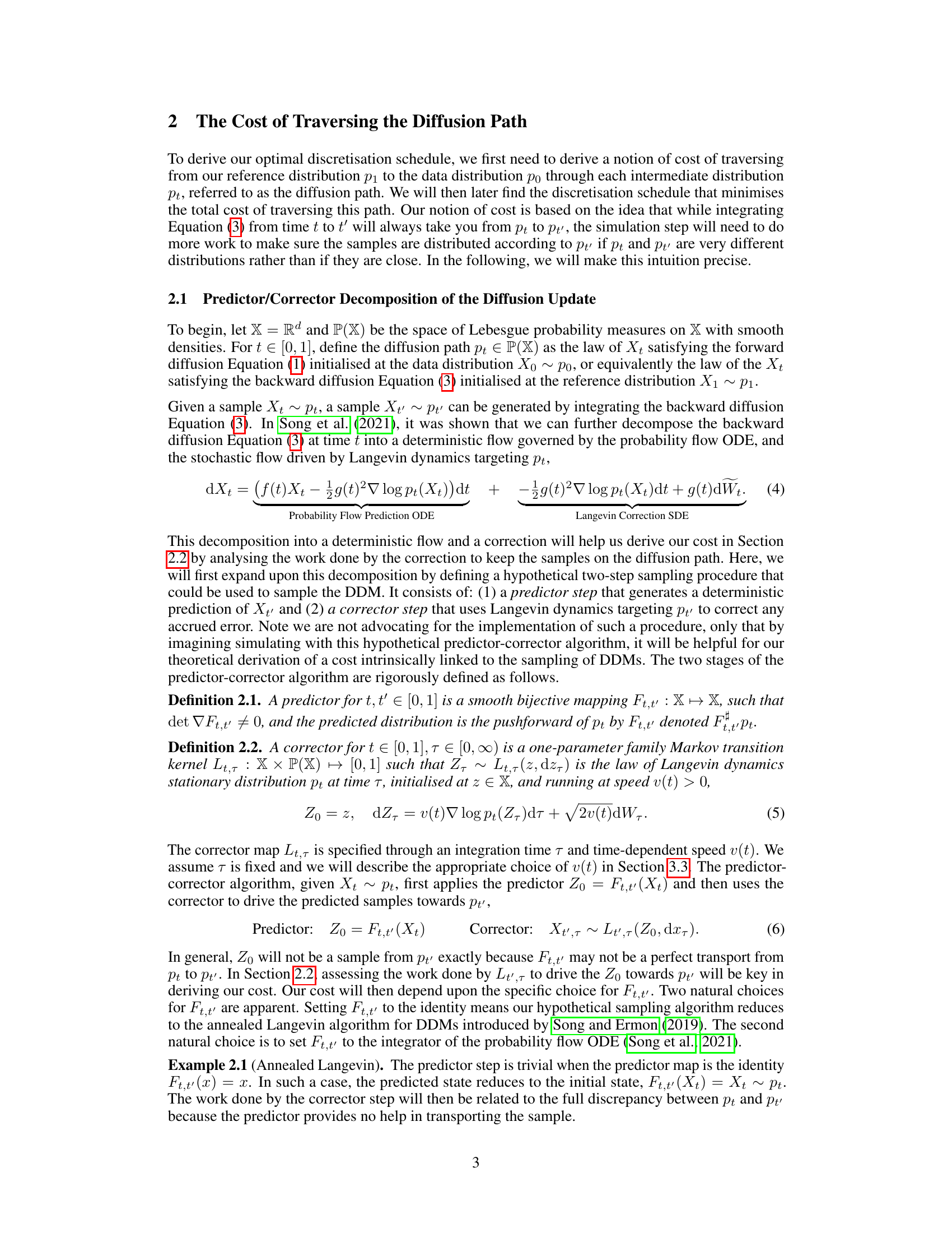
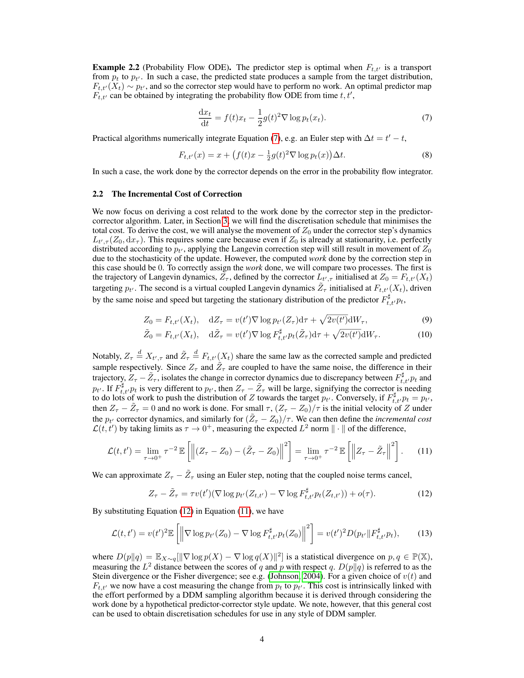
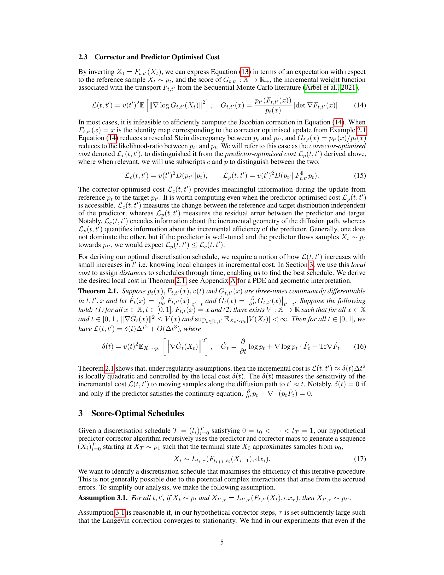
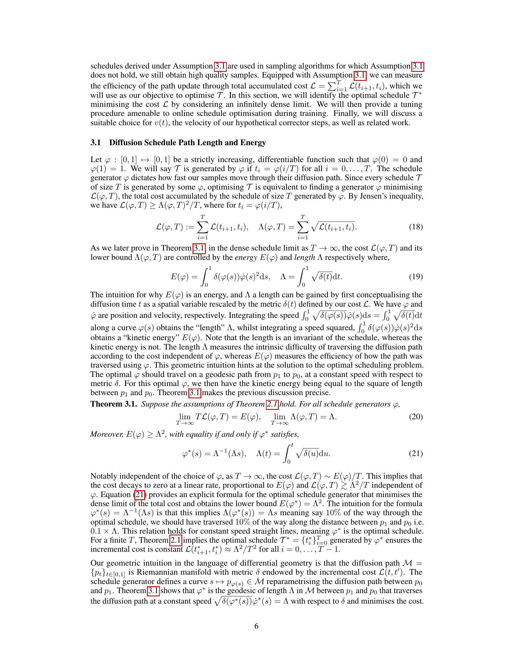
More on figures

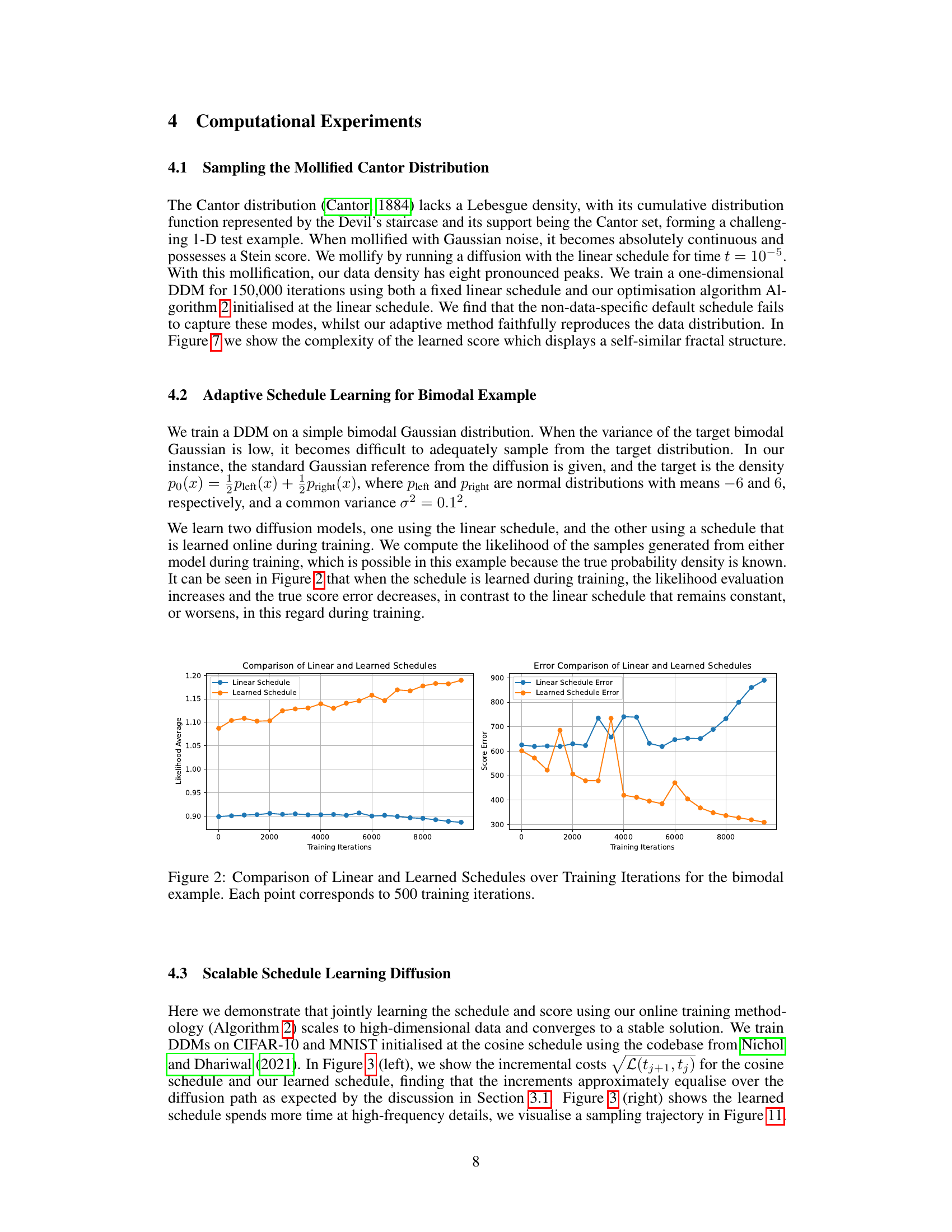
This figure compares the performance of a linear schedule and a learned schedule for training a diffusion model on a bimodal Gaussian distribution. The left panel shows the average likelihood of samples generated by the model over training iterations. The right panel displays the model’s score error, which measures the discrepancy between the model’s predicted score and the true score of the data distribution. The results show that the learned schedule leads to higher likelihoods and lower score errors compared to the linear schedule.

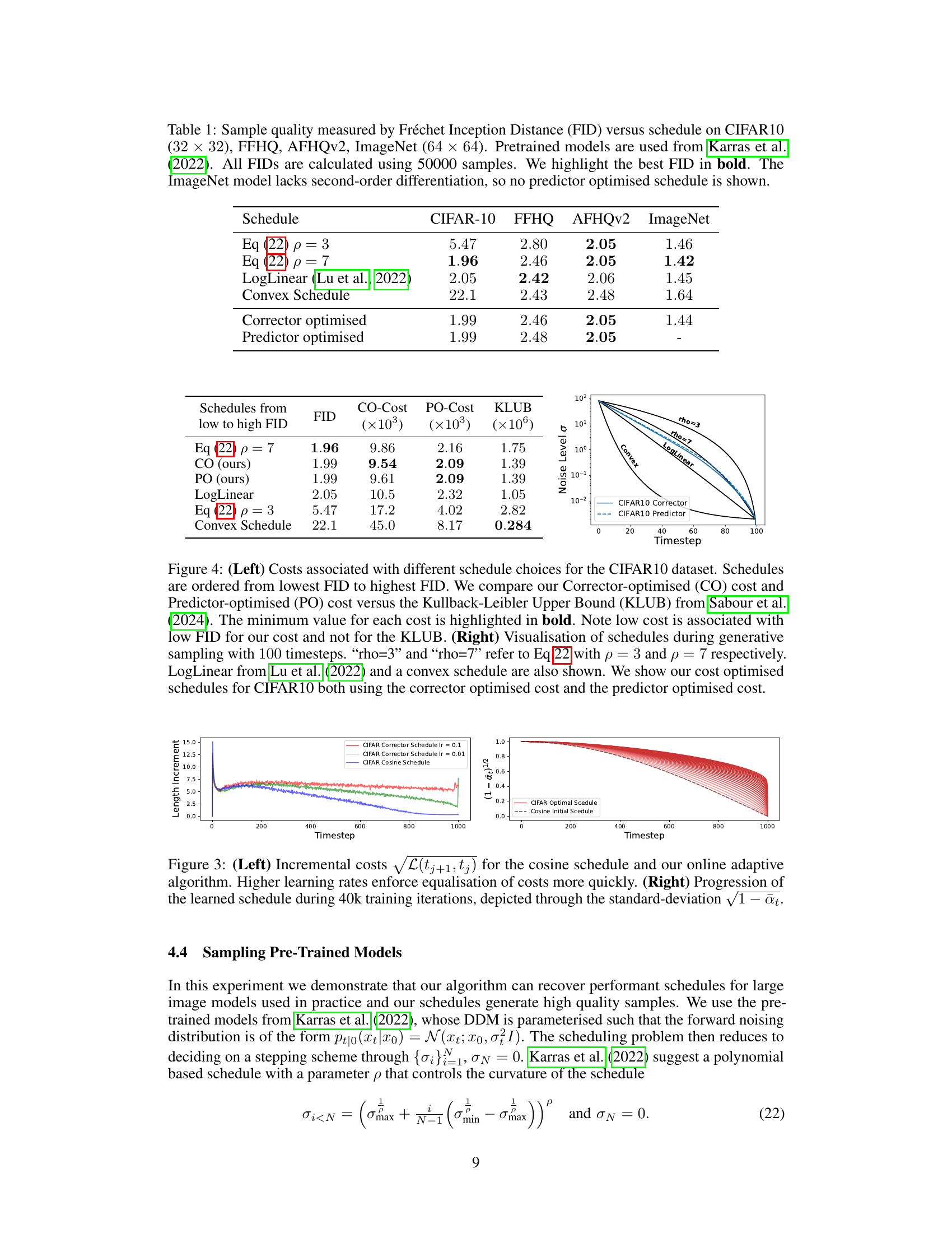
This figure shows two plots. The left plot compares the incremental costs for the cosine schedule and the online adaptive algorithm. The right plot shows the progression of the learned schedule over 40,000 training iterations, visualized by the standard deviation of the noise level.
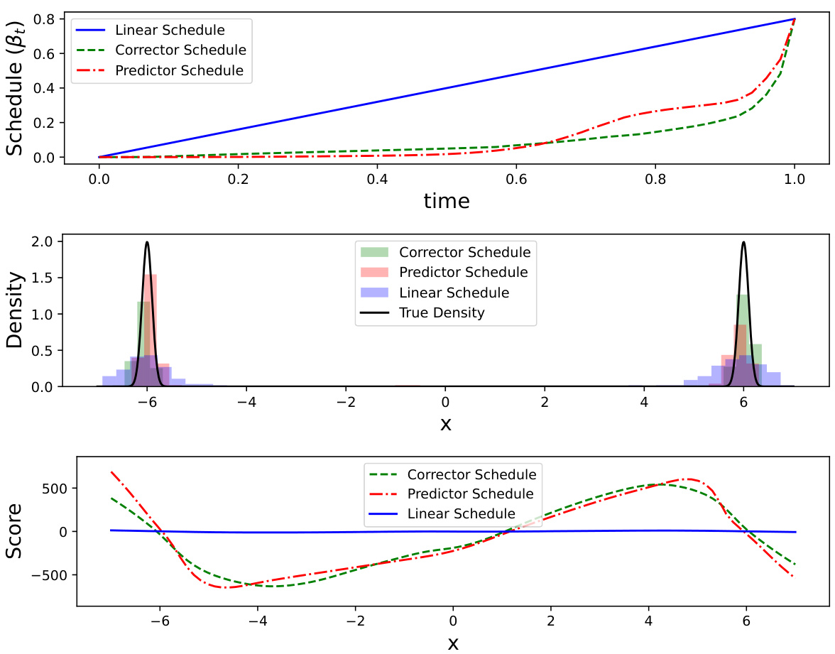
This figure compares three different schedules and their resulting density estimates for a bimodal Gaussian distribution. The top panel shows the three schedules: a linear schedule (blue), a corrector-optimized schedule (green), and a predictor-optimized schedule (red). The middle panel displays density estimates for each schedule, along with the true density of the bimodal Gaussian distribution. The bottom panel shows the score estimates for each schedule. The results show that the optimized schedules yield more accurate density estimates than the linear schedule, particularly near the modes of the distribution.

This figure compares three different schedules for a bimodal Gaussian distribution: linear, Stein score optimized, and predictor optimized. The predictor optimized schedule shows improved accuracy in estimating the true score compared to the linear schedule, leading to a more precise density estimation.
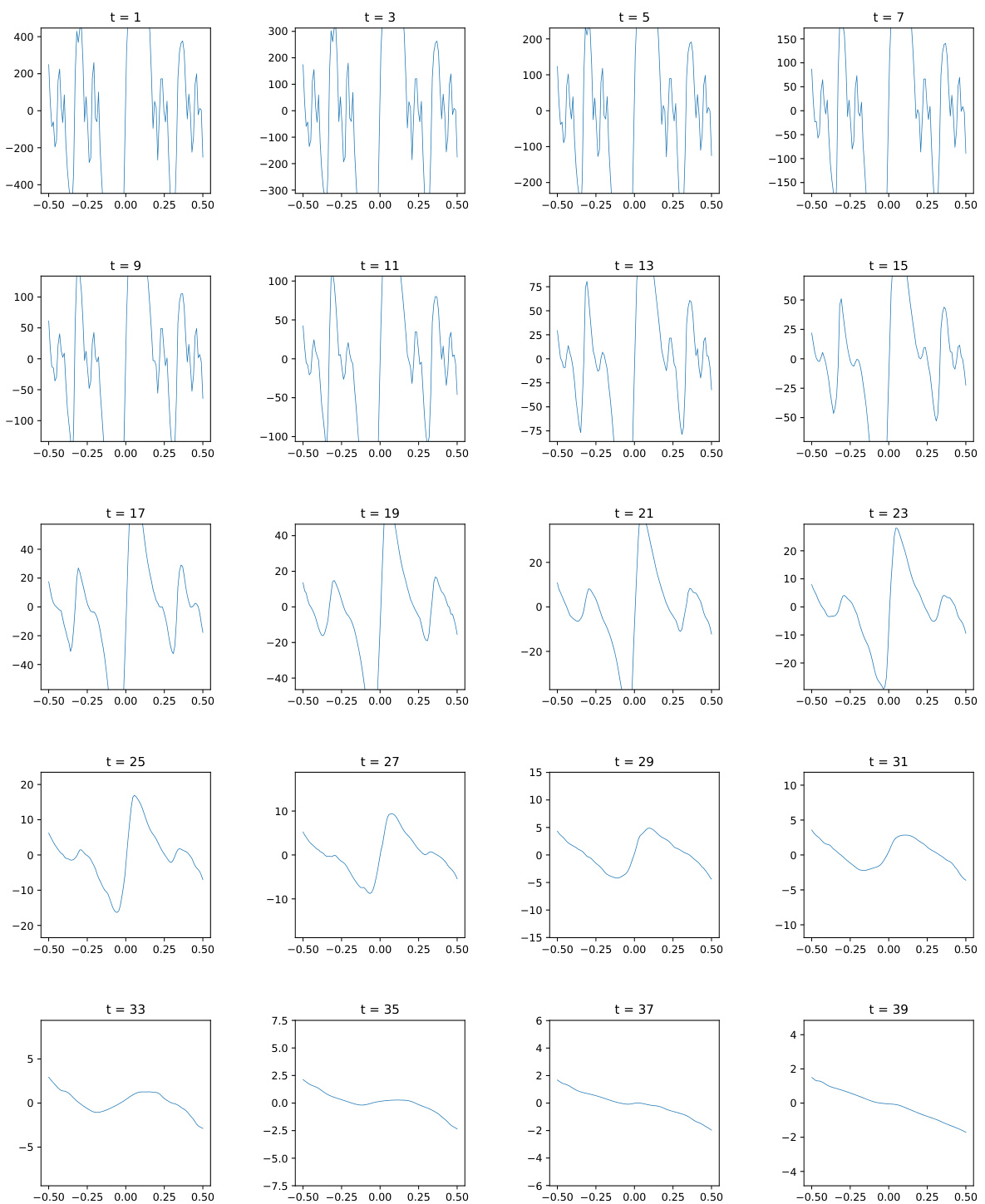
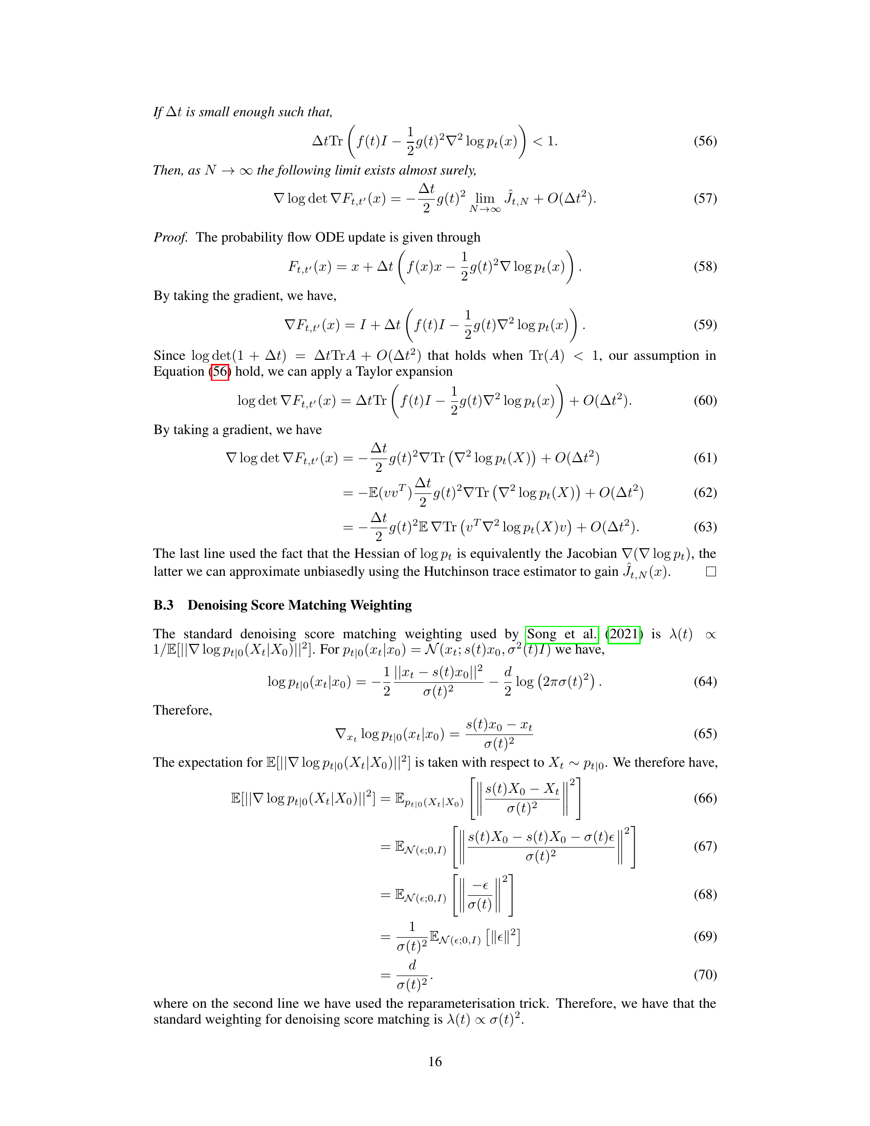
This figure shows the evolution of the estimated score for the mollified Cantor distribution across different time steps (t = 1 to t = 39). Each subplot displays the estimated score as a function of x for a specific time step. The figure highlights how the linear schedule fails to capture the multimodal nature of the distribution, unlike the corrector-optimized schedule. The self-similar fractal structure of the score is also shown, indicating the complexity of the distribution.

This figure displays the corrector and predictor optimized schedules for four different image datasets: CIFAR-10, FFHQ, AFHQv2, and ImageNet. The x-axis represents the timestep in the diffusion process, and the y-axis represents the noise level (sigma). Each dataset has two lines: one solid line representing the corrector optimized schedule and one dashed line representing the predictor optimized schedule. The schedules show how the noise level decreases over time during the sampling process. The different lines illustrate the variations in optimal scheduling strategies across different datasets with varying complexities and data characteristics. The curves show the decay of noise level in the diffusion process to yield high quality samples.
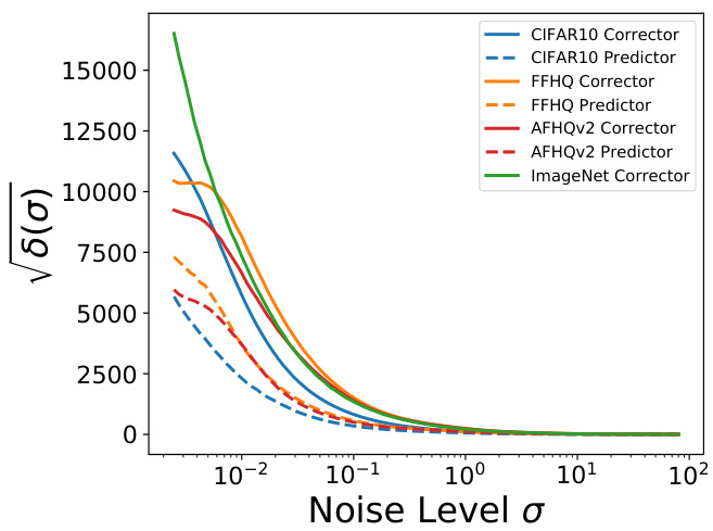
This figure displays the corrector and predictor optimized schedules for four image datasets: CIFAR10, FFHQ, AFHQv2, and ImageNet. The x-axis represents the timestep in the generative process, and the y-axis represents the noise level (σ). Each dataset has two lines: one for the corrector-optimized schedule and one for the predictor-optimized schedule. The schedules show how the noise level changes over time during the sampling process. The shapes of the curves reveal the different strategies employed to navigate the diffusion process for each dataset and optimization method.

This figure shows the progression of the length and energy of the diffusion path during the training of a MNIST model, comparing a model with adaptive schedule learning and one without. The length and energy are metrics derived from the cost function used to optimize the schedule. The figure indicates that the optimized schedule leads to a longer diffusion path, suggesting that it explores the data distribution differently compared to the fixed cosine schedule.
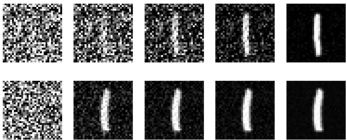
This figure compares the sample generation process using a standard cosine schedule and the optimized schedule proposed in the paper. The top row shows samples generated using the cosine schedule, which spends more time near the Gaussian reference distribution. The bottom row shows samples generated using the optimized schedule, which quickly identifies large-scale features and focuses more on the data distribution.

This figure shows the progression of length and energy during the training process of a MNIST model with and without adaptive schedule learning. The length and energy increase during training. The optimized schedule results in a larger length value, suggesting a difference in the learned diffusion path compared to the fixed schedule.
More on tables

This table presents the Fréchet Inception Distance (FID) scores, a measure of sample quality, for different sampling schedules on four image datasets: CIFAR-10, FFHQ, AFHQv2, and ImageNet. The schedules compared include those from prior work (Equation (22) with p=3 and p=7, LogLinear) and the novel corrector and predictor-optimized schedules proposed in the paper. Lower FID scores indicate better sample quality. The results show that the proposed optimized schedules achieve FID scores competitive with or better than the best-performing schedule from prior work. The ImageNet results exclude the predictor-optimized schedule due to the model’s limitations.

This table compares the Fréchet Inception Distance (FID) scores, a metric for evaluating the quality of generated images, across different scheduling methods for four image datasets: CIFAR-10, FFHQ, AFHQv2, and ImageNet. The schedules compared include those derived from the paper’s proposed methods (Corrector and Predictor Optimized) as well as existing methods (LogLinear, and schedules from Karras et al. 2022). Lower FID scores indicate higher quality images. The results show that the proposed methods achieve competitive performance compared to the existing schedules.

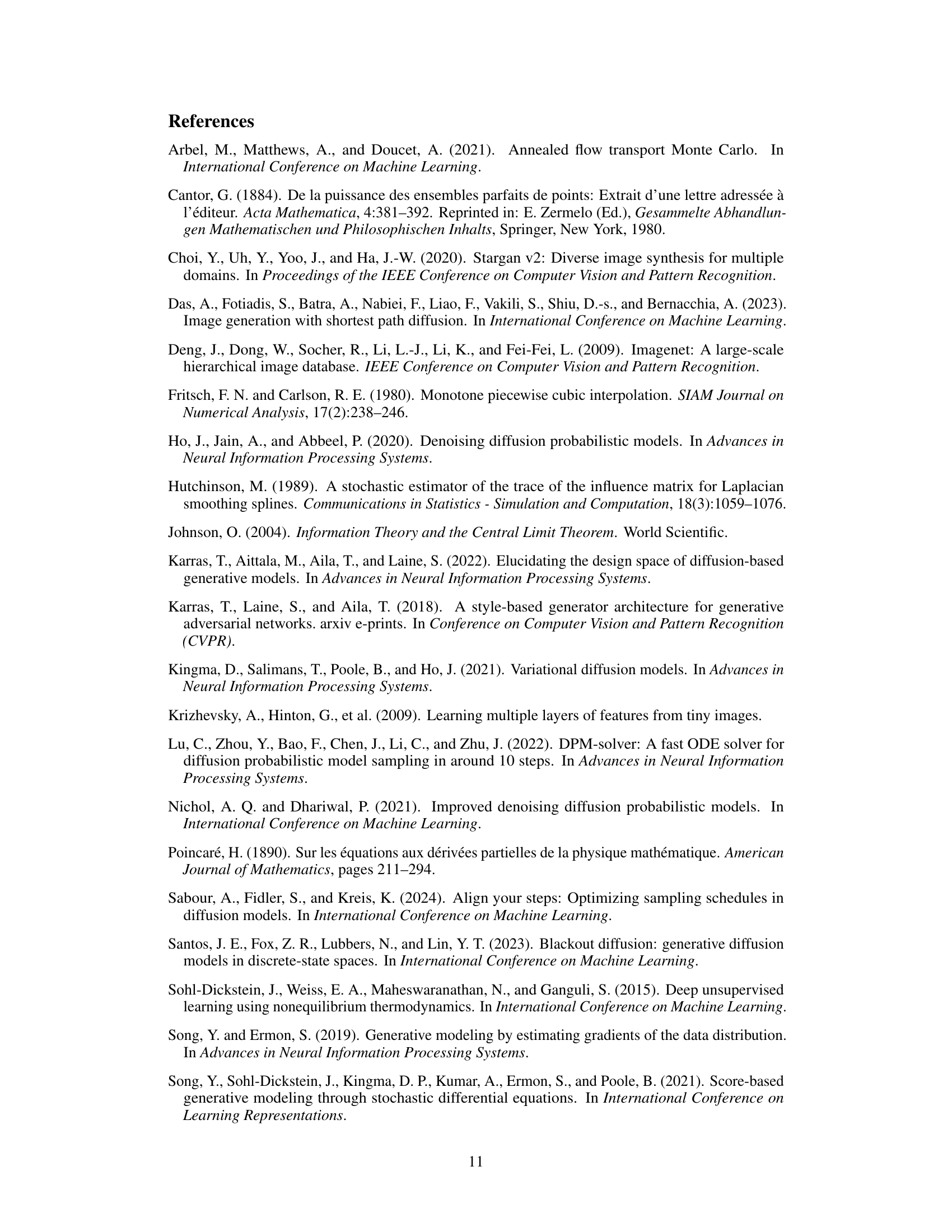
This table shows how the number of discretisation points, T, used during sampling affects the quality of generated samples for different schedules. It demonstrates that the FID (Fréchet Inception Distance, a metric for image quality) decreases with increasing T for all schedules. However, when T is small (low resolution), only the optimised schedules maintain stable performance, indicating improved efficiency.

This table presents the sFID (a measure of sample quality) achieved by different sampling schedules on the CIFAR-10 dataset. Different numbers of discretization points (T) were used with each schedule, to analyze how the number of discretization points affects the quality of the generated samples. The schedules include the corrector-optimized schedule from the proposed algorithm, and three other schedules based on varying values of the parameter ρ (3, 7, and 100).
Full paper#


