TL;DR#
Current knowledge distillation (KD) methods primarily focus on convolutional neural networks (CNNs) and struggle with transferring knowledge between different architectures, especially when using large pre-trained vision transformers (ViTs) as teachers. This paper addresses these limitations by exploring the scalability of using ViTs as powerful teachers for diverse student models.
The authors introduce ScaleKD, a novel method that combines three core components to effectively transfer knowledge: cross-attention projection to align feature computation, dual-view feature mimicking to capture nuanced knowledge, and teacher parameter perception to transfer pre-training knowledge. ScaleKD achieves state-of-the-art results across multiple datasets and architectures, demonstrating significant performance improvements and scalability when using larger teacher models and datasets. It also provides a more efficient alternative to intensive pre-training, saving considerable time and computational resources.
Key Takeaways#
Why does it matter?#
This paper is crucial because it challenges the conventional wisdom in knowledge distillation by demonstrating the effectiveness of strong, pre-trained vision transformers as teachers for diverse student architectures. This opens new avenues for efficient model training, reducing reliance on expensive pre-training, and improving the performance of various architectures. The findings are significant for researchers aiming to improve model efficiency and scalability across different deep learning architectures.
Visual Insights#

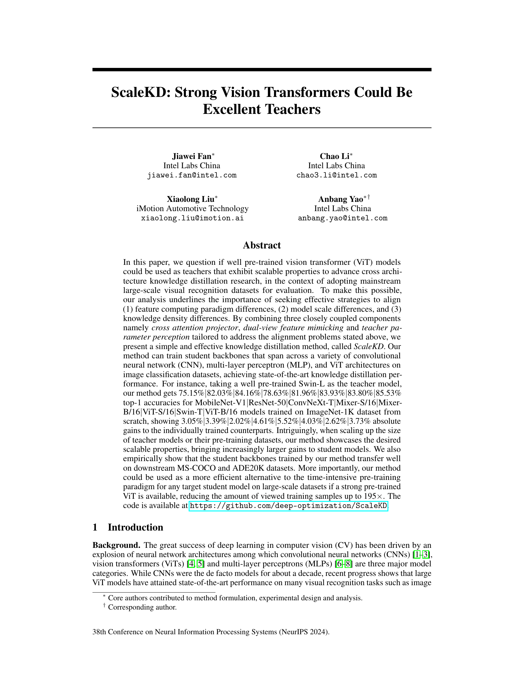
🔼 This figure illustrates the three core components of the ScaleKD method: Cross Attention Projector (CAP), Dual-view Feature Mimicking (DFM), and Teacher Parameter Perception (TPP). CAP aligns the feature computing paradigms of the teacher and student models by using positional embeddings and a cross-attention mechanism. DFM mimics the teacher’s features in both the original and frequency domains to address model scale differences. TPP aligns the parameter spaces of the teacher and student by creating a proxy feature processing path. Importantly, the teacher model remains frozen during the distillation process, and no modifications are made to the student model during inference.
read the caption
Figure 1: Overview of three core components in our ScaleKD, which are (a) cross attention projector, (b) dual-view feature mimicking, and (c) teacher parameter perception. Note that the teacher model is frozen in the distillation process and there is no modification to the student's model at inference.
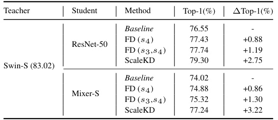
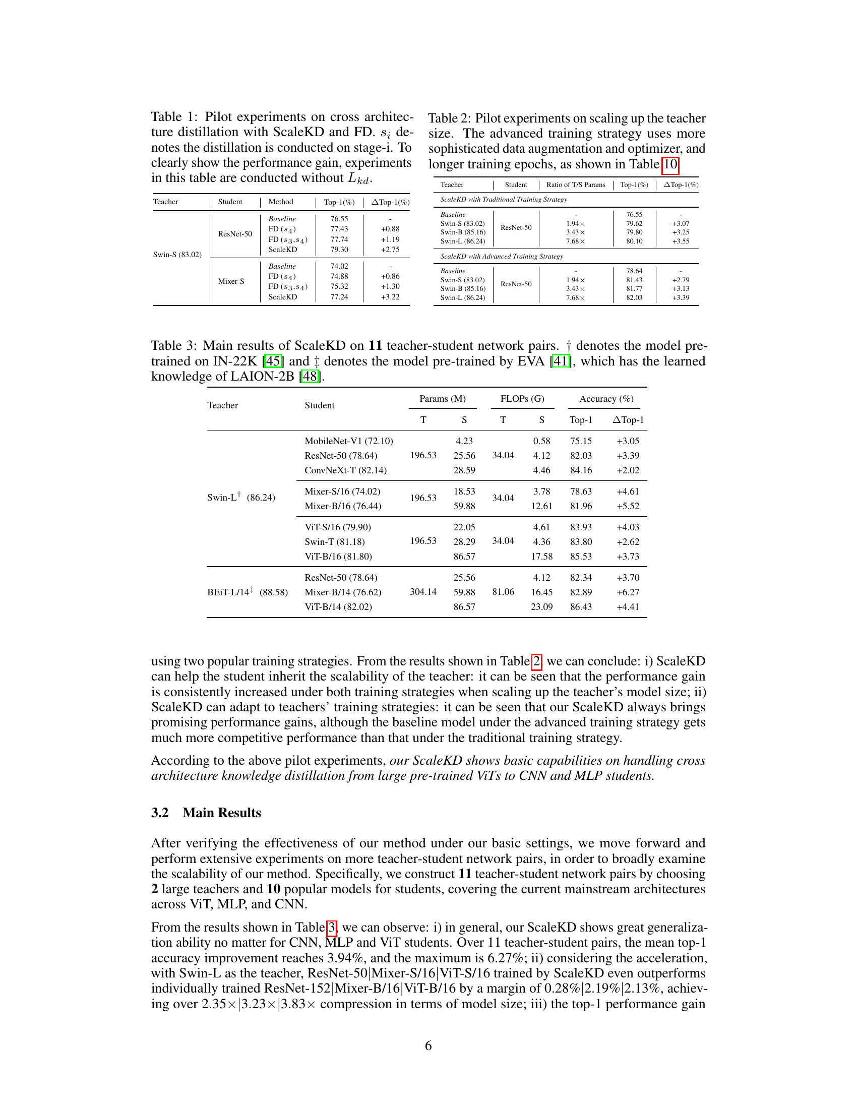
🔼 This table presents the results of pilot experiments comparing ScaleKD and traditional Feature Distillation (FD) methods on cross-architecture knowledge distillation tasks. It shows the top-1 accuracy achieved on ResNet-50 and Mixer-S student models when using Swin-S as the teacher model. The results demonstrate that ScaleKD significantly outperforms FD, highlighting its effectiveness in bridging architectural differences for knowledge transfer.
read the caption
Table 1: Pilot experiments on cross architecture distillation with ScaleKD and FD. si denotes the distillation is conducted on stage-i. To clearly show the performance gain, experiments in this table are conducted without Lkd.
In-depth insights#
ScaleKD: KD with ViTs#
ScaleKD presents a novel approach to knowledge distillation (KD) leveraging the power of pre-trained Vision Transformers (ViTs) as teachers. The core idea revolves around bridging the inherent differences between ViT architectures and various student networks (CNNs, MLPs, other ViTs). This is achieved through a three-pronged strategy: a cross-attention projector for feature paradigm alignment, dual-view feature mimicking to address scale and knowledge density discrepancies, and teacher parameter perception to transfer pre-training knowledge. ScaleKD demonstrates state-of-the-art performance, significantly boosting student accuracy across diverse architectures and showcasing scalability when using larger teachers or pre-training datasets. The method’s effectiveness is further validated through transfer learning experiments. Overall, ScaleKD offers a compelling alternative to time-consuming ViT pre-training, particularly when a strong pre-trained ViT model is readily available.
Cross-Arch KD#
Cross-architecture knowledge distillation (Cross-Arch KD) presents a significant challenge and opportunity in deep learning. It tackles the problem of transferring knowledge from a teacher model with one architecture (e.g., Vision Transformer) to a student model with a different architecture (e.g., Convolutional Neural Network). This is crucial because different architectures possess unique strengths and weaknesses; transferring knowledge effectively enables leveraging these strengths while mitigating weaknesses. Key challenges involve aligning feature representations, handling differences in model capacity and complexity, and addressing varying knowledge densities learned during pre-training. Effective Cross-Arch KD methods need to cleverly bridge these architectural disparities, potentially employing techniques like feature adaptation modules, intermediate representation spaces, or specialized loss functions to ensure knowledge transfer is faithful and beneficial. Successful Cross-Arch KD significantly improves the efficiency of training models, allowing smaller or less computationally expensive student networks to achieve performance comparable to much larger teacher networks. This has major implications for resource-constrained applications and edge deployments. Future research could explore more advanced alignment techniques, better handling of architectural variations beyond CNNs and ViTs, and the development of methods that explicitly quantify and measure the quality and fidelity of the knowledge transfer.
Scalable Teacher#
The concept of a “Scalable Teacher” in knowledge distillation is crucial for efficiently leveraging large, pre-trained models. A scalable teacher model should exhibit consistent performance improvements as its size or training data increases. This scalability enables transfer of increasingly refined knowledge to student models, leading to significant gains even for smaller student networks. Effective alignment strategies are critical for bridging the inherent differences in feature computation paradigms and model scales between teacher and student. The teacher’s capacity to scale allows for adaptability across diverse student architectures (CNNs, MLPs, ViTs) and provides a path for enhancing generalization performance beyond the dataset on which the student is trained. Addressing knowledge density differences becomes important if the teacher’s extensive training data isn’t accessible to the student; a scalable teacher can compensate for that limitation by implicitly transferring rich, generalized knowledge.
Feature Mimicking#
Feature mimicking in knowledge distillation aims to transfer knowledge from a teacher model to a student model by aligning their feature representations. Effective feature mimicking requires careful consideration of several factors: the choice of teacher and student architectures, the types of features used (e.g., intermediate layer activations, output logits), and the method employed to measure and enforce feature similarity (e.g., mean squared error, KL-divergence). A well-designed feature mimicking strategy should account for differences in model capacity and knowledge density between teacher and student, ensuring that the student effectively learns and generalizes from the teacher’s knowledge. Successful feature mimicking often involves more than a simple direct comparison of features. Advanced techniques, such as attention-based mechanisms or feature transformation, can help bridge architectural differences and focus on the most relevant features for knowledge transfer. The effectiveness of feature mimicking is ultimately assessed through performance gains on downstream tasks.
Future of KD#
The future of knowledge distillation (KD) hinges on addressing its current limitations and exploring new frontiers. Scaling KD to larger models and datasets is crucial, requiring innovative techniques to handle increased computational demands and the complexity of knowledge transfer. Bridging the architecture gap between teacher and student networks will be vital, possibly through more sophisticated feature alignment and knowledge representation methods. Developing more efficient KD algorithms is also important, reducing computational cost and improving training efficiency. Furthermore, research into theoretical understanding of KD will provide a stronger foundation for future advancements. This includes a deeper understanding of what constitutes transferable knowledge and how to effectively extract and transfer it between disparate models. Finally, exploring novel applications of KD beyond model compression, such as enhancing robustness and generalization, will unlock its full potential.
More visual insights#
More on figures

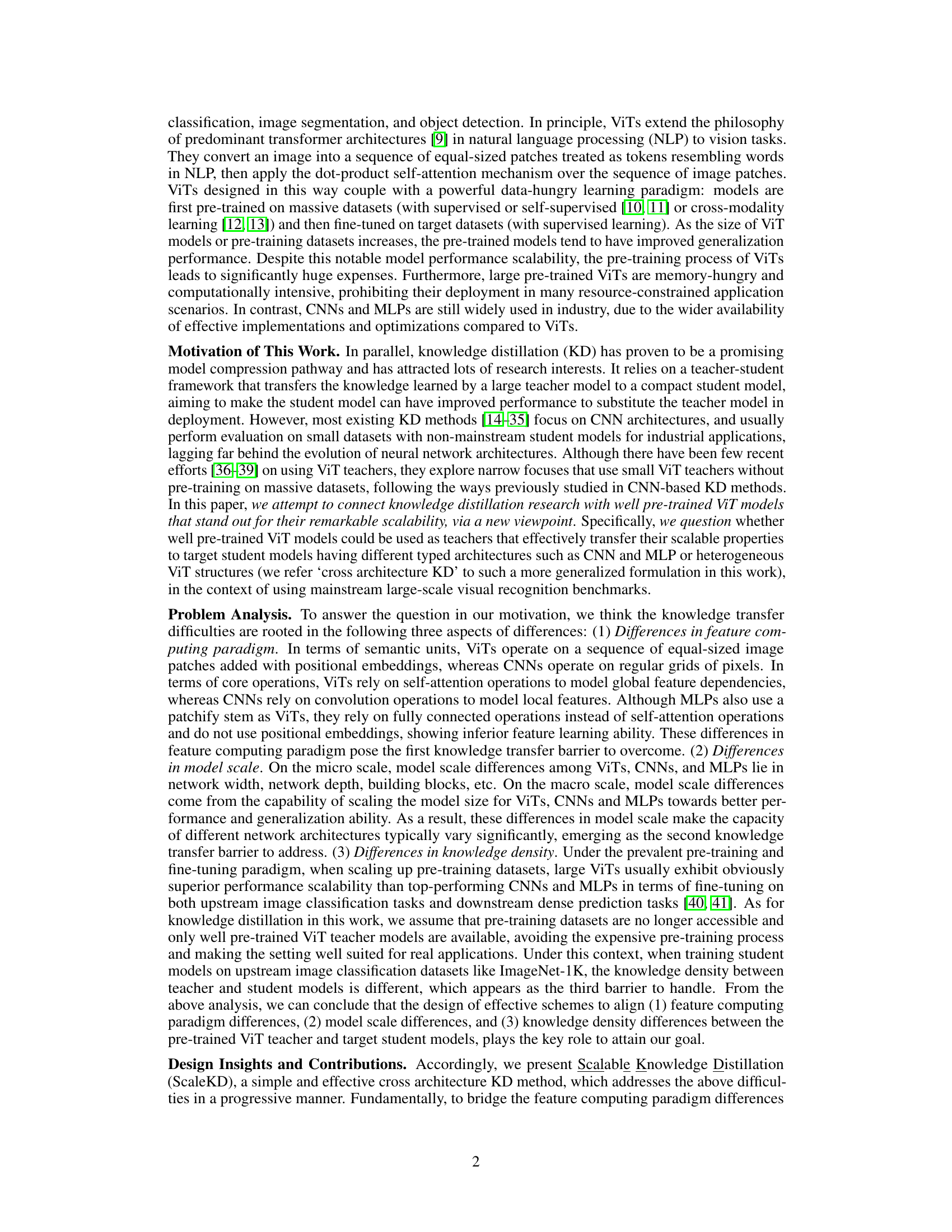
🔼 This figure shows the frequency distribution of features from a BEIT-L/14 model in the frequency domain. The dominant response is concentrated in the direct component (zero frequency), indicating an imbalance in the feature distribution. More detailed explanation of how this visualization was generated is found in Figure 5.
read the caption
Figure 2: Feature distribution of BEIT-L/14 [41] in the frequency domain, where the direct component response is dominant. Details on drawing this figure are shown in Figure 5.

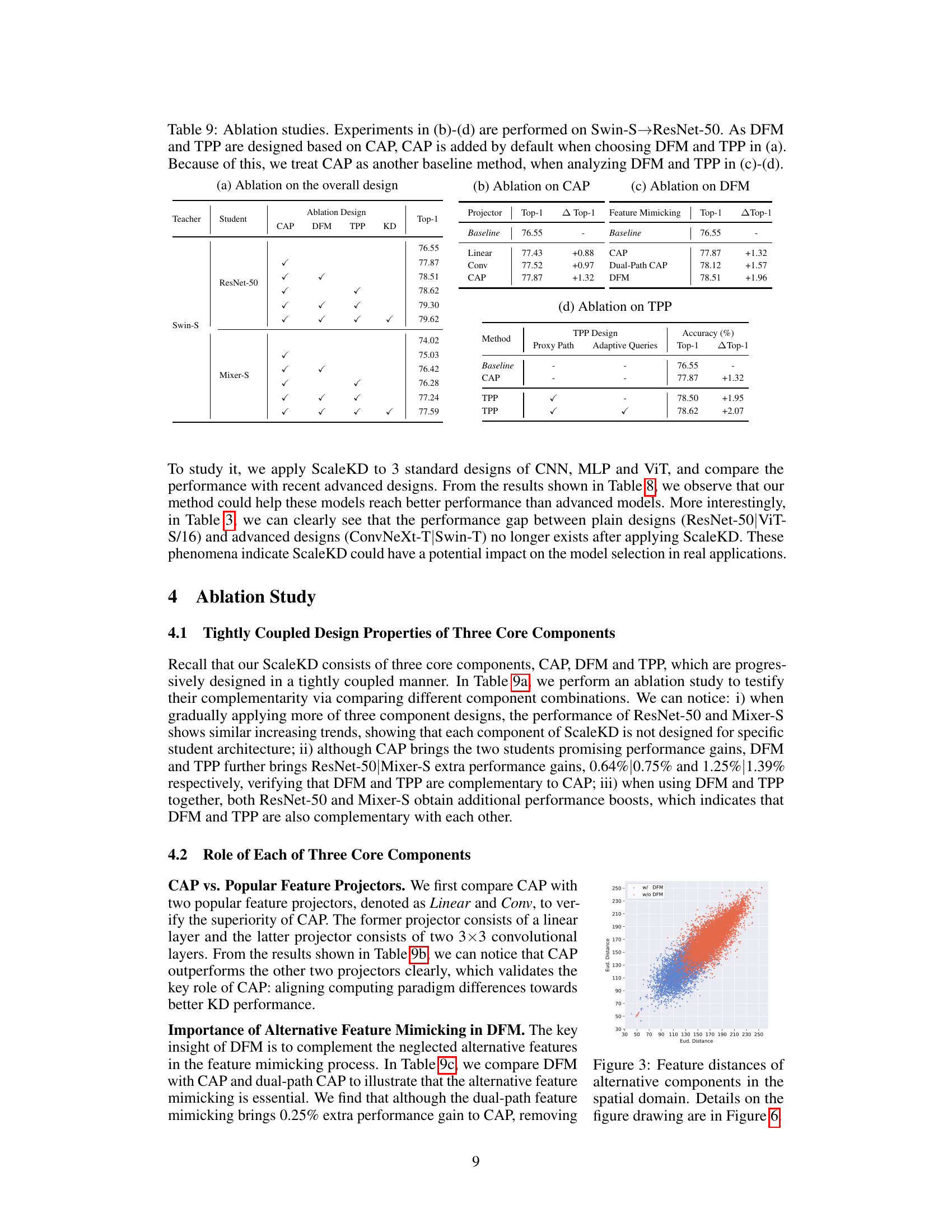
🔼 This figure shows the feature distance distributions between teacher and student models with and without DFM applied. The high-dimensional feature distances are projected into a 2D space for visualization. The results demonstrate that DFM effectively reduces the distance between the teacher and student features, particularly for the alternative components, which are often neglected in traditional knowledge distillation methods.
read the caption
Figure 6: Feature distance distributions of alternative components for the last stage features between teacher and student on IN-1K. We obtain 64,000 feature pairs on Swin-L→ResNet-50 network pair from 64,000 samples. After calculating the distance between teacher and student, we project the high-dimension distances into a two-dimension space for illustration. Finally, we randomly select 6,400 data points for 8 times to draw the scatters. Blue points denote the distances without DFM, while orange points denote the distances with DFM.

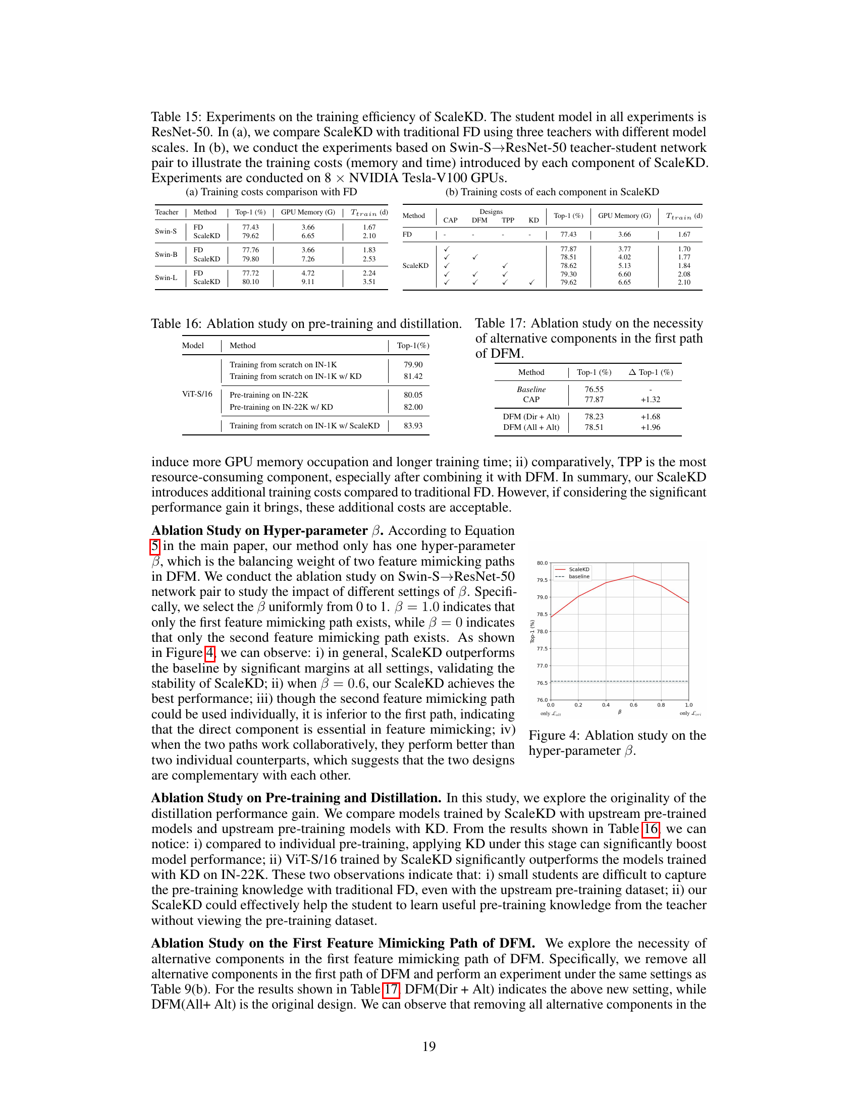
🔼 This ablation study shows the impact of the hyperparameter β on the performance of ScaleKD. β controls the balance between two feature mimicking paths in DFM. The x-axis represents the value of β, ranging from 0.0 (only using alternative features) to 1.0 (only using direct component). The y-axis shows the top-1 accuracy on the ResNet-50 student model. The results indicate that a balance between both paths (around β = 0.6) leads to optimal performance, outperforming using either path alone.
read the caption
Figure 4: Ablation study on the hyper-parameter β.

🔼 This figure shows the frequency distributions of feature maps from three different large pre-trained vision transformers (ViTs): ViT-L/14, Swin-L, and BEIT-L/14. The data used is a subset of ImageNet-1K (IN-1K). Each subfigure represents a 3D plot showing frequency distribution on a per-channel basis. The process involves extracting feature maps, applying a Discrete Cosine Transform (DCT) to each channel, averaging across samples, and displaying the magnitude of the frequency response. This visualization helps to illustrate the differences in feature distributions between these pre-trained ViTs, highlighting the relative importance of different frequency components in their feature representations.
read the caption
Figure 5: More illustrative feature distributions of large pre-trained ViTs in the frequency domain. We first collect the output feature maps of 1600 samples from IN-1K, then conduct DCT on each channel, and finally take the average value across these samples after converting all responses into absolute values.

🔼 This figure illustrates the three main components of the ScaleKD method: the Cross Attention Projector (CAP), Dual-view Feature Mimicking (DFM), and Teacher Parameter Perception (TPP). CAP aligns the feature computing paradigms of the teacher and student models. DFM mimics features from two perspectives: the original space and a frequency-filtered space to address model scale and knowledge density differences. TPP bridges the parameter spaces of teacher and student by using feature mimicking in a proxy path. Importantly, the teacher model remains frozen during the distillation process, and no modifications are made to the student model for inference.
read the caption
Figure 1: Overview of three core components in our ScaleKD, which are (a) cross attention projector, (b) dual-view feature mimicking, and (c) teacher parameter perception. Note that the teacher model is frozen in the distillation process and there is no modification to the student's model at inference.
More on tables
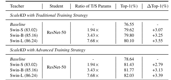
🔼 This table presents the results of pilot experiments designed to evaluate the impact of scaling up the size of the teacher model on the performance of the ScaleKD method. Two training strategies are compared: a traditional strategy and an advanced strategy (details in Table 10). The table shows the baseline performance, the teacher-student model parameter ratio, and the resulting top-1 accuracy gains achieved by ScaleKD with both strategies. The results demonstrate the scalability of the ScaleKD approach, showing improved gains as the teacher model size is increased.
read the caption
Table 2: Pilot experiments on scaling up the teacher size. The advanced training strategy uses more sophisticated data augmentation and optimizer, and longer training epochs, as shown in Table 10.

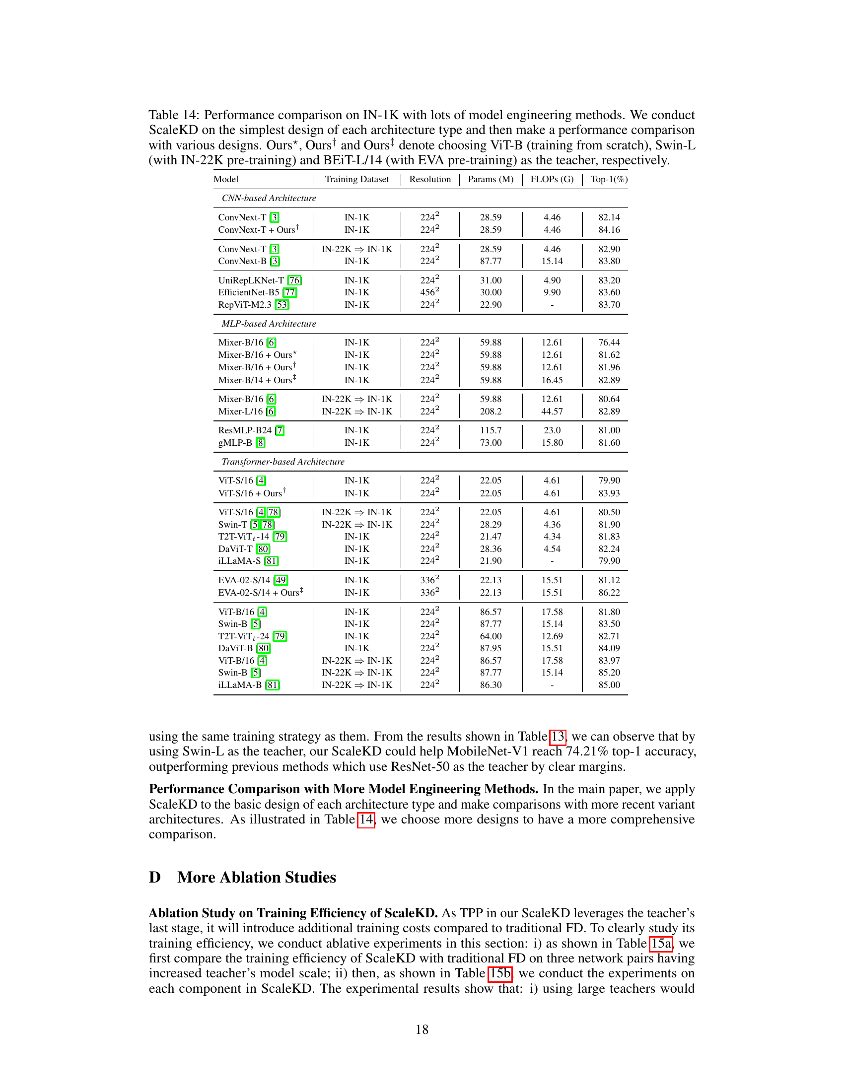
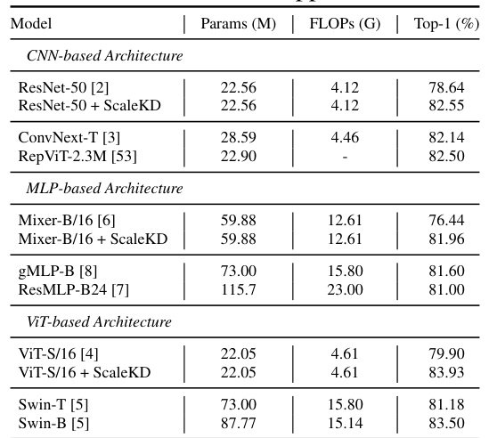
🔼 This table presents the main results of the ScaleKD method. It shows the top-1 accuracy and the improvement achieved by ScaleKD compared to individually trained counterparts for 11 different teacher-student network pairs. The teacher models are large vision transformers (ViTs), while the student models represent a variety of architectures including CNNs, MLPs, and other ViTs. The table also indicates which models were pre-trained on larger datasets (IN-22K or LAION-2B).
read the caption
Table 3: Main results of ScaleKD on 11 teacher-student network pairs. † denotes the model pre-trained on IN-22K [45] and ‡ denotes the model pre-trained by EVA [41], which has the learned knowledge of LAION-2B [48].
🔼 This table presents the transfer learning results on the MS-COCO dataset. It shows the performance of different models (ResNet-50, Swin-T, and ViT-B/16) pre-trained using various methods (baselines and the proposed ScaleKD) on three downstream tasks: classification, object detection, and instance segmentation. The results demonstrate the generalization capability of models trained by ScaleKD.
read the caption
Table 5: Transfer learning results (%) on MS-COCO.

🔼 This table presents the transfer learning results on the MS-COCO dataset. It compares the performance of baseline models (ResNet-50 and Swin-T) with those trained using the ScaleKD method. The results are shown for classification (IN-1K), object detection, and instance segmentation tasks, indicating the improvements achieved by ScaleKD in downstream tasks. The metrics shown include Top-1 accuracy for classification and Average Precision (AP) and its variants for object detection and instance segmentation.
read the caption
Table 5: Transfer learning results (%) on MS-COCO.
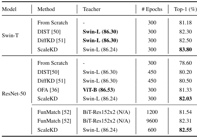
🔼 This table compares the performance of ScaleKD against other state-of-the-art knowledge distillation (KD) methods. The comparison uses ResNet-50 and Swin-T as student models, trained with the advanced training strategy. The table highlights ScaleKD’s superior performance, even with fewer training epochs compared to other methods, showcasing its efficiency in transferring knowledge from a strong pre-trained Vision Transformer (ViT) teacher.
read the caption
Table 7: Performance comparison with recent top-performing KD methods. Following the settings of them, the students are trained under the advanced training strategy. Best results are bolded.
🔼 This table presents the main results of the ScaleKD knowledge distillation method. It shows the top-1 accuracy and the improvement achieved by ScaleKD on ImageNet-1K for 11 different teacher-student network pairs. The table includes various architectures (CNN, MLP, and ViT) and model sizes. It highlights the significant performance gains obtained using ScaleKD, especially when compared to individually training the student models from scratch.
read the caption
Table 3: Main results of ScaleKD on 11 teacher-student network pairs. † denotes the model pre-trained on IN-22K [45] and ‡ denotes the model pre-trained by EVA [41], which has the learned knowledge of LAION-2B [48].

🔼 This table presents the transfer learning results on the MS-COCO dataset. It compares the performance of baseline models (ResNet-50 and Swin-T) against models trained using the ScaleKD method. The results are shown for image classification (top-1 accuracy), object detection (average precision - AP), and instance segmentation (average precision - AP). The numbers in parentheses indicate the improvement in performance achieved by using ScaleKD.
read the caption
Table 5: Transfer learning results (%) on MS-COCO.
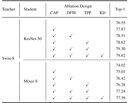
🔼 This table presents the ablation study results for the three core components of ScaleKD: CAP, DFM, and TPP. It shows the impact of each component individually and in combination on the model’s performance. The experiment was conducted on the Swin-S to ResNet-50 teacher-student pair. The table systematically evaluates different combinations to reveal the individual contributions and the synergistic effects of the three core components.
read the caption
Table 9: Ablation studies. Experiments in (b)-(d) are performed on Swin-S→ResNet-50. As DFM and TPP are designed based on CAP, CAP is added by default when choosing DFM and TPP in (a). Because of this, we treat CAP as another baseline method, when analyzing DFM and TPP in (c)-(d).
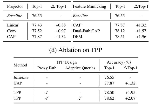
🔼 This table presents the ablation study results for the three core components of ScaleKD: Cross Attention Projector (CAP), Dual-view Feature Mimicking (DFM), and Teacher Parameter Perception (TPP). It shows the impact of each component individually and in combination on the overall performance, demonstrating their complementary nature. The experiments are conducted using a Swin-S teacher and ResNet-50 student model.
read the caption
Table 9: Ablation studies. Experiments in (b)-(d) are performed on Swin-S→ResNet-50. As DFM and TPP are designed based on CAP, CAP is added by default when choosing DFM and TPP in (a). Because of this, we treat CAP as another baseline method, when analyzing DFM and TPP in (c)-(d).
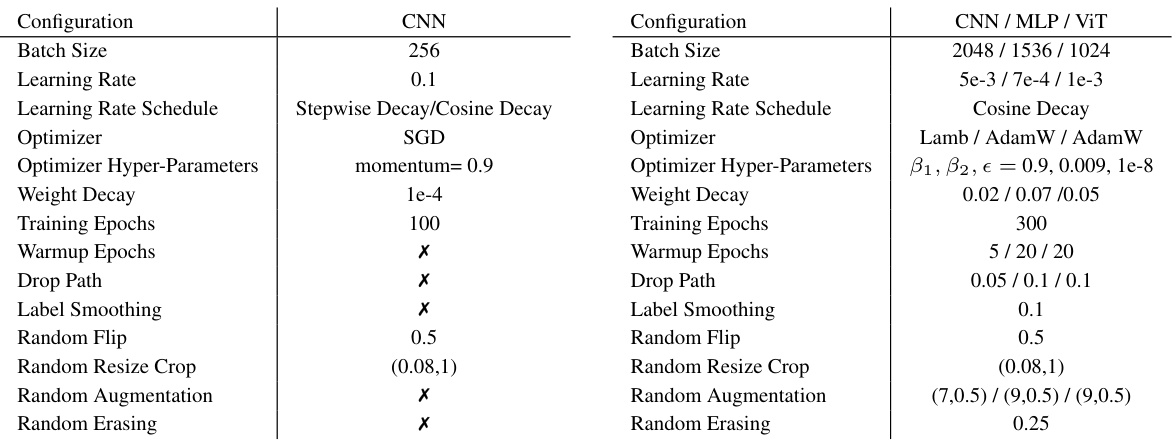
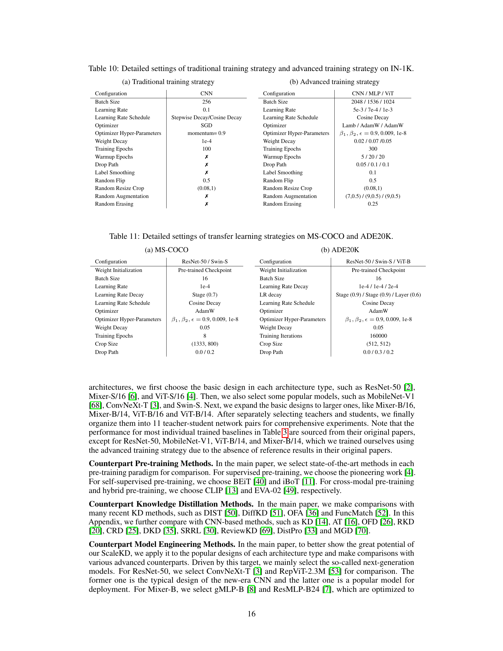
🔼 This table details the configurations used for training the models on the ImageNet-1K dataset. It compares two training strategies: a traditional one, commonly used in previous knowledge distillation research and an advanced strategy used for more recently developed CNNs, MLPs, and Vision Transformers (ViTs). The table lists various hyperparameters such as batch size, learning rate, learning rate schedule, optimizer, weight decay, and data augmentation techniques for both strategies.
read the caption
Table 10: Detailed settings of traditional training strategy and advanced training strategy on IN-1K.

🔼 This table details the configurations used for transfer learning experiments on the MS-COCO and ADE20K datasets. It specifies settings for both datasets, including weight initialization, batch size, learning rate and its decay schedule, optimizer, hyper-parameters, weight decay, training epochs (or iterations), crop size, and drop path rate. These settings are crucial for replicating and understanding the results of the transfer learning experiments reported in the paper. The table showcases two different experimental set ups, one for the MS-COCO dataset and another one for the ADE20K dataset. The differences highlight the adaptation of hyper-parameters based on dataset requirements and the different tasks involved (object detection/instance segmentation vs. semantic segmentation).
read the caption
Table 11: Detailed settings of transfer learning strategies on MS-COCO and ADE20K.

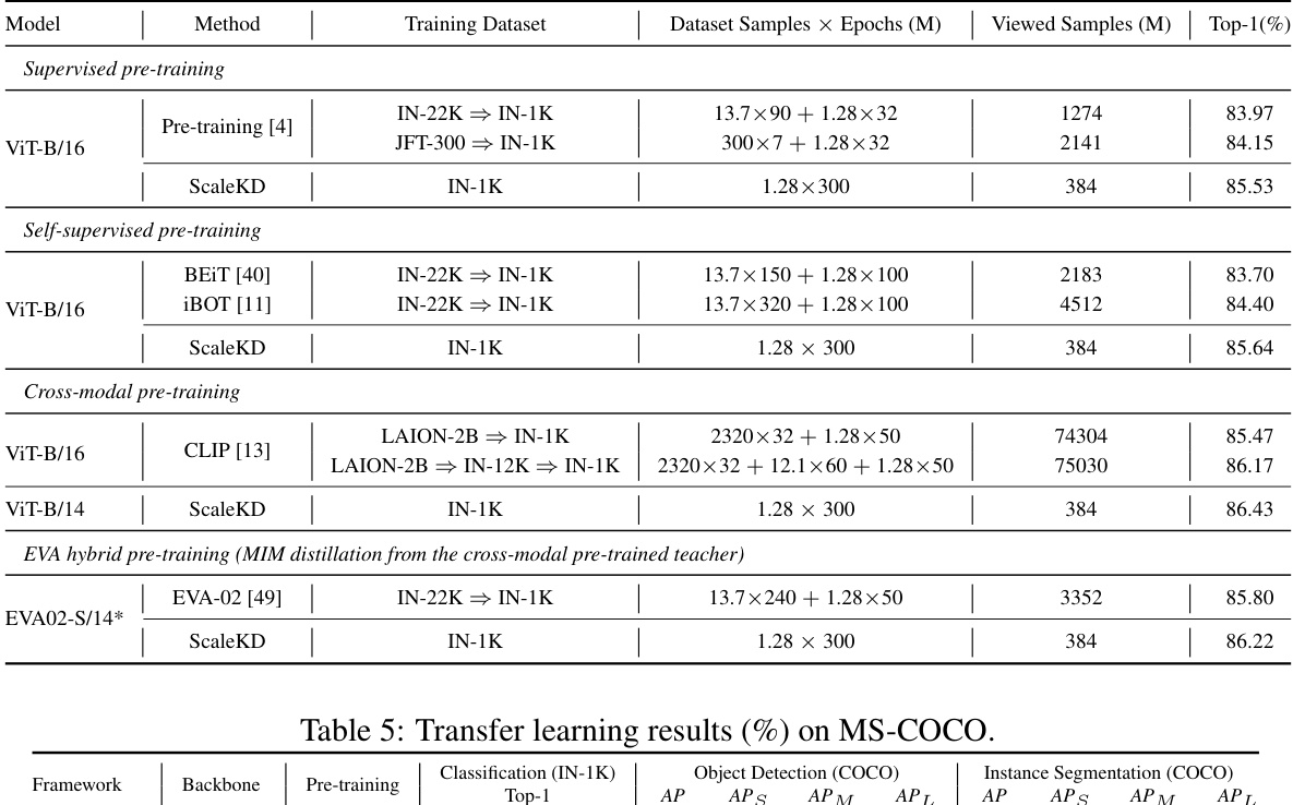
🔼 This table presents the results of experiments designed to investigate whether ScaleKD enables student models to inherit the scalability properties of their teacher models, specifically focusing on the impact of the teacher’s pre-training data. The table compares the performance of student models trained using ScaleKD against baselines representing various pre-training methods (supervised, self-supervised, cross-modal, and hybrid). The results show that ScaleKD consistently achieves better performance than the baselines, even when the student model only sees data from ImageNet-1k, demonstrating the transfer of pre-training knowledge.
read the caption
Table 4: Experiments on exploring scalable properties from the teacher's pre-training data. We use the best reported models with different pre-training methods as our baselines to examine whether our student model has learned the teacher's pre-training knowledge. We use Swin-L as the teacher for the first two experiments and BEiT-L/14 as the teacher for the rest two experiments. ⇒ denotes transfer learning and * denotes the model is trained and tested with 384× 384 sample resolution.

🔼 This table presents the main results of the ScaleKD method on ImageNet-1K. It compares the top-1 accuracy of 11 different student models trained using ScaleKD with their respective baselines (individually trained models). The student models represent diverse architectures, including MobileNet-V1, ResNet-50, ConvNeXt-T, Mixer-S/16, Mixer-B/16, ViT-S/16, Swin-T, and ViT-B/16. The teacher models used are Swin-L and BEIT-L/14. The table highlights the improvement in top-1 accuracy achieved by ScaleKD for each student model compared to its individually trained counterpart. It also shows the model size (parameters and FLOPs) for both teacher and student models. Additionally, the table notes which teacher models were pre-trained on larger datasets (IN-22K or LAION-2B).
read the caption
Table 3: Main results of ScaleKD on 11 teacher-student network pairs. † denotes the model pre-trained on IN-22K [45] and ‡ denotes the model pre-trained by EVA [41], which has the learned knowledge of LAION-2B [48].

🔼 This table presents the main results of the ScaleKD method on eleven different teacher-student network pairs. It shows the top-1 accuracy achieved by each student model when trained using ScaleKD, along with the parameters and FLOPs for both the teacher and student models. Some teacher models were pre-trained on larger datasets (indicated by † and ‡). The table demonstrates the effectiveness of ScaleKD across various architectures and pre-training scenarios.
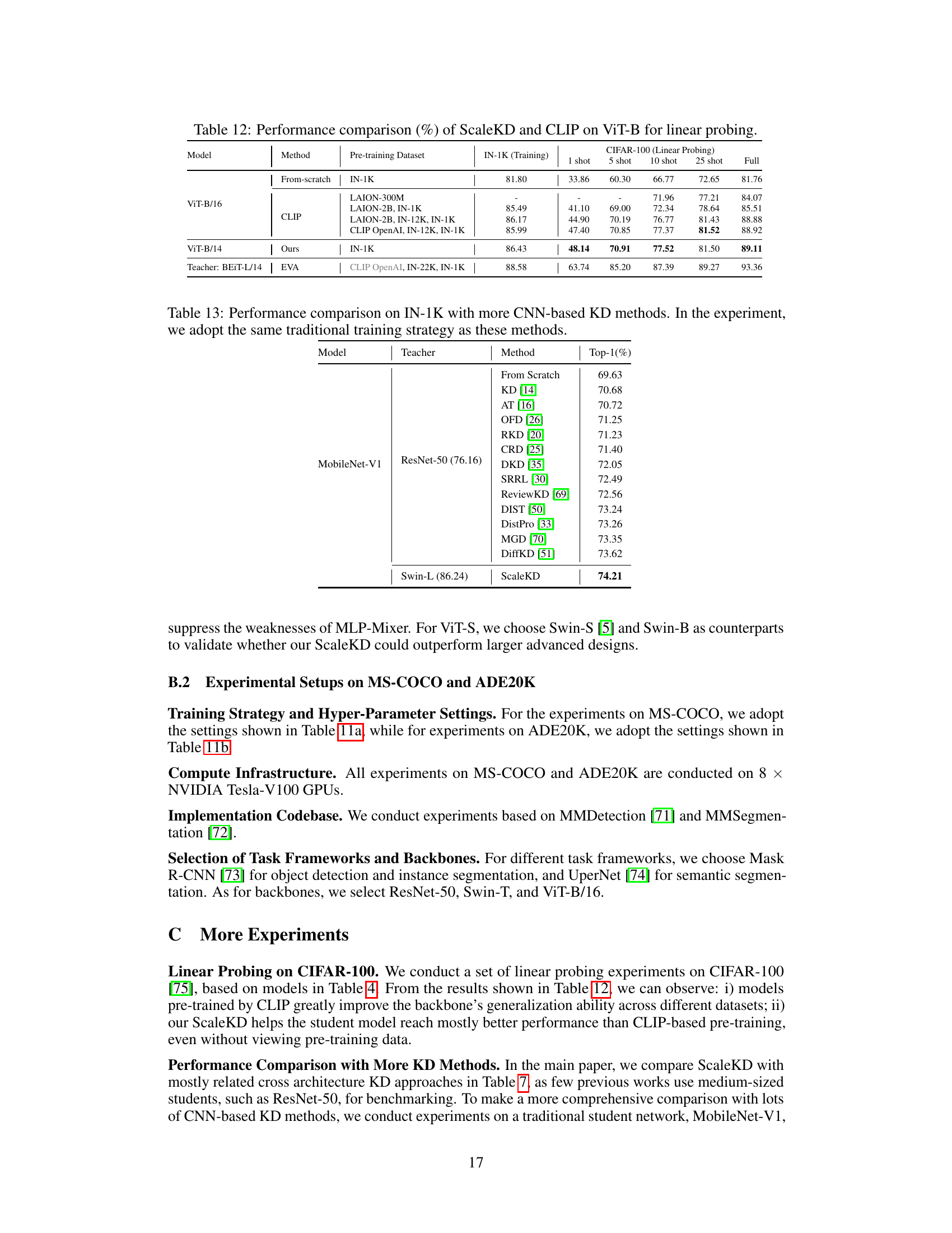
read the caption
Table 3: Main results of ScaleKD on 11 teacher-student network pairs. † denotes the model pre-trained on IN-22K [45] and ‡ denotes the model pre-trained by EVA [41], which has the learned knowledge of LAION-2B [48].
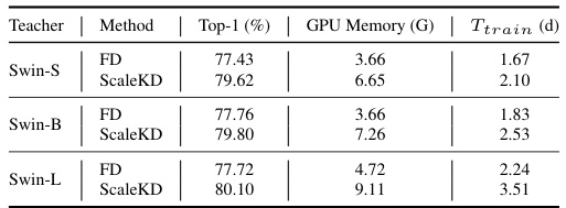
🔼 This table presents an ablation study on the training efficiency of ScaleKD, comparing it with traditional feature distillation (FD). It shows the GPU memory usage and training time in days for different teacher models (Swin-S, Swin-B, and Swin-L) using both FD and ScaleKD. A further breakdown examines the impact of each ScaleKD component (CAP, DFM, TPP) on training efficiency.
read the caption
Table 15: Experiments on the training efficiency of ScaleKD. The student model in all experiments is ResNet-50. In (a), we compare ScaleKD with traditional FD using three teachers with different model scales. In (b), we conduct the experiments based on Swin-S→ResNet-50 teacher-student network pair to illustrate the training costs (memory and time) introduced by each component of ScaleKD. Experiments are conducted on 8 × NVIDIA Tesla-V100 GPUs.

🔼 This table presents an ablation study on the training efficiency of the ScaleKD method. It compares the training costs (GPU memory and time) of ScaleKD against traditional Feature Distillation (FD) using three different teacher models with varying sizes. It also breaks down the training costs of ScaleKD into its individual components (CAP, DFM, TPP, KD) to assess their contribution to the overall cost.
read the caption
Table 15: Ablation study on training efficiency of ScaleKD. The student model in all experiments is ResNet-50. In (a), we compare ScaleKD with traditional FD using three teachers with different model scales. In (b), we conduct the experiments based on Swin-S→ResNet-50 teacher-student network pair to illustrate the training costs (memory and time) introduced by each component of ScaleKD. Experiments are conducted on 8 × NVIDIA Tesla-V100 GPUs.
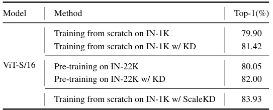
🔼 This ablation study compares the performance of training a ViT-S/16 model from scratch on ImageNet-1K, with and without knowledge distillation (KD), and compares those results with pre-training on ImageNet-22K, with and without KD. It demonstrates that ScaleKD significantly improves performance compared to other methods.
read the caption
Table 16: Ablation study on pre-training and distillation.
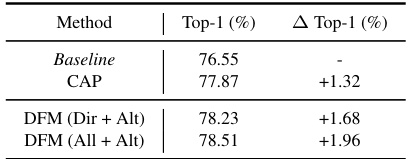
🔼 This table presents ablation study results evaluating the contribution of each component (CAP, DFM, TPP) of the ScaleKD method. Experiments were conducted on the Swin-S to ResNet-50 teacher-student pair. The table shows the impact of each component on the final Top-1 accuracy. CAP is a baseline, with DFM and TPP progressively added to assess their individual and combined contributions.
read the caption
Table 9: Ablation studies. Experiments in (b)-(d) are performed on Swin-S→ResNet-50. As DFM and TPP are designed based on CAP, CAP is added by default when choosing DFM and TPP in (a). Because of this, we treat CAP as another baseline method, when analyzing DFM and TPP in (c)-(d).
Full paper#
