↗ OpenReview ↗ NeurIPS Homepage ↗ Chat
TL;DR#
Current data valuation methods focus on individual datasets, neglecting the value of the underlying data distribution. This is problematic for applications such as data marketplaces where buyers need to evaluate data distributions based on limited sample previews from different vendors. The heterogeneity (i.e. differences) across the distributions further complicates the valuation process.
This research introduces a novel MMD-based valuation method that directly addresses this challenge. By using the maximum mean discrepancy (MMD) to measure the difference between data distributions and their samples, and adopting the Huber model to account for data heterogeneity, the authors created an actionable policy for comparing distributions. Their empirical results showcase the method’s sample efficiency and effectiveness in identifying valuable data distributions across various datasets and applications.
Key Takeaways#
Why does it matter?#
This paper is crucial for researchers in data markets and machine learning. It provides theoretically-grounded and actionable policies for comparing data distributions, addressing a critical gap in existing data valuation methods. The MMD-based approach is sample-efficient and effective, offering significant improvements over existing baselines. Further investigation into its theoretical properties, especially its connection to incentive compatibility, and extensions to more complex heterogeneity models will be of significant interest.
Visual Insights#

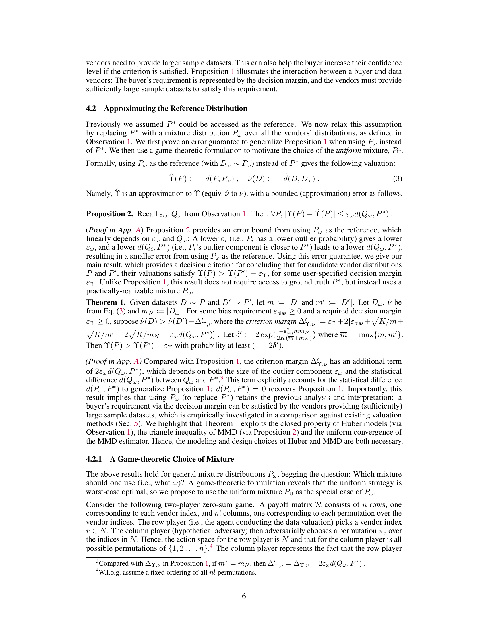
This figure shows the sample efficiency comparison of different data valuation methods. Three metrics, namely l2 error, l∞ error, and the number of inversions, are plotted against the sample size (as a percentage of the total sample size m). The results demonstrate that the MMD-based method (Ours) is more sample-efficient, meaning it converges to the true values faster with smaller sample sizes, compared to other methods such as CS, DAVINZ, LAVA, and MMD2.

This table compares four different distance metrics (KL divergence, Wasserstein distance, squared MMD, and MMD) across five criteria: sample complexity (asymptotic and finite sample bounds), computational complexity, whether the triangle inequality holds, and whether it is compatible with the Huber model. The comparison helps to justify the choice of MMD as the best distance metric for data distribution valuation in this paper.
In-depth insights#
Distrib. Data Value#
The concept of “Distributional Data Value” represents a significant advancement in data valuation, moving beyond the assessment of individual datasets to encompass the inherent value within the underlying data distribution. This shift is crucial because it acknowledges that the value of a dataset is not solely determined by its contents, but also by the broader context from which it’s sampled. This approach enables a more nuanced understanding of data value, especially in scenarios involving data marketplaces and vendor selection. A key advantage is the ability to compare data distributions effectively even with limited sample sizes, making it practical for real-world applications. The methodology also addresses challenges of data heterogeneity, providing robust and theoretically-grounded methods for valuation, which are supported by empirical evidence. Overall, the concept of ‘Distributional Data Value’ offers a more robust and future-proof approach to data valuation that considers the underlying data-generating processes and enables informed decision-making in diverse settings.
MMD-Based Valuation#
The core of this research paper revolves around a novel data valuation method based on the Maximum Mean Discrepancy (MMD). MMD provides a robust way to compare the similarity of probability distributions, even when only sample data is available, a crucial aspect when dealing with the heterogeneity of data across different vendors. The proposed MMD-based valuation directly addresses the challenge of comparing data distributions by quantifying their dissimilarity from a reference distribution, making it particularly suitable for evaluating the usefulness of data from multiple sources. The theoretical underpinnings of this method are rigorously established, providing error guarantees and actionable policies for comparing distributions based on sample datasets. Empirical results demonstrate its sample efficiency and effectiveness in real-world settings, showcasing significant advantages over existing baselines in identifying high-value data distributions. The use of a Huber model to capture data heterogeneity further strengthens the theoretical framework. Overall, this MMD-based approach offers a theoretically-grounded and practically-effective solution for data valuation, offering new insights for data market analysis and resource allocation.
Huber Heterogeneity#
The concept of “Huber Heterogeneity” in data valuation addresses the realistic scenario where data distributions from different vendors are not identical. It leverages the Huber contamination model, a mixture model representing the true data distribution and an outlier component, to capture this heterogeneity. This framework is crucial because it allows for a theoretically grounded comparison of data distributions even when the underlying true distribution is unknown. The Huber model’s strength lies in providing a structured way to quantify and analyze the impact of this heterogeneity on the valuation process. By using this model, the researchers can mathematically characterize the effect of the outlier component and its deviation from the true distribution on the overall value of the data, ultimately enabling theoretically principled data valuation methods and actionable policies for data buyers.
Sample Efficiency#
The research paper investigates sample efficiency in data distribution valuation, focusing on how effectively different valuation methods estimate the value of data distributions using limited sample datasets. The authors demonstrate that their proposed Maximum Mean Discrepancy (MMD)-based method is sample-efficient compared to several baselines. This efficiency is crucial because, in real-world scenarios, access to complete datasets might be limited or costly. The empirical results highlight that MMD outperforms other approaches, especially when dataset sizes are small, providing robust and accurate value estimations. Theoretical guarantees supporting the sample efficiency are derived, offering a principled and actionable policy for comparing data distributions based on sample data. The results are robust across various datasets and downstream tasks, further strengthening the claims of sample efficiency. This efficient valuation approach is vital for data markets, where buyers assess data quality based on small previews, and for applications requiring effective value assessments despite data scarcity.
Future Directions#
The research paper’s findings on data distribution valuation offer exciting avenues for future exploration. Extending the theoretical framework beyond the Huber model to accommodate broader forms of data heterogeneity is crucial. This involves developing robust methods that can handle diverse data patterns and still provide theoretically sound and actionable policies for data valuation. Another important direction is developing and analyzing incentive-compatible mechanisms for data markets that incentivize truthful data reporting. This is particularly challenging in the absence of a ground truth reference distribution and necessitates the development of game-theoretic models that account for strategic behavior among data vendors. The investigation of the practical limits of sample efficiency and the development of techniques to handle extremely high-dimensional data remain significant research objectives. Finally, the integration of various aspects of data valuation—including data utility, privacy, and fairness—into a unified framework is a crucial step towards building robust and responsible data markets. The development of these comprehensive models will be fundamental to creating effective and ethical data valuation policies.
More visual insights#
More on figures

This figure shows the sample efficiency comparison of different data valuation methods. The y-axis represents three different metrics: L2 error, L∞ error, and the number of inversions. The x-axis shows the sample size as a percentage of the total sample size (m=10000). The lower the values on the y-axis for a given sample size, the better the performance of the method. The figure demonstrates that the proposed MMD-based method (Ours) converges faster (i.e., is more sample-efficient) than other baselines.

This figure compares the sample efficiency of different data valuation methods. The y-axis shows three different metrics measuring the error in the estimated valuation: l2 error, l∞ error, and the number of inversions. The x-axis shows the sample size as a percentage of the total sample size (m=10000). The plot shows that the MMD-based method proposed by the authors converges more quickly than other methods as the sample size increases. This suggests that the MMD-based method requires fewer samples to achieve a good approximation of the true data distribution value.

This figure compares the sample efficiency of different data valuation methods. The y-axis shows three different criteria for evaluating the accuracy of the methods: l2 error, l∞ error, and the number of inversions. The x-axis shows the sample size as a percentage of the total sample size (m=10000). The plot shows how quickly each method converges to the true value as the sample size increases. A method that converges quickly is considered to be more sample-efficient.

This figure compares the sample efficiency of several baseline methods against the proposed MMD-based method in terms of three criteria: l2 error, l∞ error, and the number of inversions. The x-axis represents the sample size as a percentage of the maximum sample size (m=10000). The y-axis shows the values for each criterion. Lower values indicate better performance. The figure shows that the MMD-based method converges more quickly than the baseline methods, suggesting higher sample efficiency. The experiment uses the MNIST and EMNIST datasets.

This figure shows the correlation between the valuation scores obtained using the proposed MMD-based method (Eq. (5)) and the actual error levels (MMD distance between the vendor’s distribution and the ground truth). The four plots represent different numbers of vendors (n = 100, 200, 500, 1000). Each point represents a vendor, with the x-coordinate being the error and the y-coordinate being the valuation. The orange lines are linear regressions showing a strong positive correlation (R-squared = 1.00 and p-value = 0.00 for all plots), indicating that higher valuation scores correspond to lower error levels, as expected.
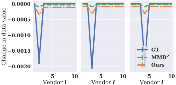
This figure shows the change in data values for each vendor when one vendor is mis-reporting. The x-axis represents the vendor index (1 to 5), and the y-axis represents the change in the data value for that vendor when mis-reporting occurs. Three methods, GT, MMD², and Ours, are compared. The results suggest that mis-reporting causes a decrease in the value for the mis-reporting vendor (i.e. negative change in data value), supporting the incentive compatibility properties of the methods.
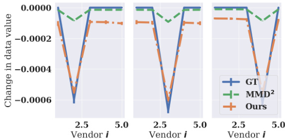
The figure shows the change in data values for five vendors (n=5) when one of them is misreporting. The x-axis represents the vendor index, and the y-axis shows the change in data value. The lines represent the ground truth (GT), MMD2, and the proposed method (Ours). The plot shows that when a vendor is misreporting, their data value decreases, while the values of the other vendors remain largely unchanged, suggesting that the proposed valuation method satisfies incentive compatibility.

This figure shows the change in data values for different vendors when one vendor misreports (adds Gaussian noise to their data). The x-axis represents the vendor index, and the y-axis shows the change in the data value (calculated using three different methods, including the ground truth and two approximation methods). The figure demonstrates that when a vendor misreports, their data value decreases, suggesting that the proposed method satisfies approximate incentive compatibility.

This figure shows the change in data values for five vendors (n=5) when one vendor misreports by adding Gaussian noise to its data. The y-axis represents the change in data value, calculated as the difference between the data value when a vendor misreports and the data value when no vendor misreports. The x-axis represents the vendor index. The plot compares the change in data values obtained using three different methods: ground truth (GT), MMD², and the proposed MMD-based method (Ours). The results indicate that misreporting leads to a decrease in data value, suggesting that the proposed method satisfies approximate incentive compatibility.
This figure demonstrates the sample efficiency of different data valuation methods by plotting three criteria (l2 error, l∞ error, and number of inversions) against the sample size. The goal is to assess how quickly each method’s valuation converges to its true value as the sample size increases. The results show that MMD-based method is generally the most sample-efficient.
More on tables
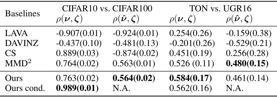
This table presents the Pearson correlation coefficients between the rankings of data sample values (obtained from various valuation methods) and the rankings of the true data distribution values for classification tasks. Higher correlation indicates better agreement between the rankings produced by a method and the true rankings of the distributions. The table includes results for two pairs of datasets: CIFAR10 vs. CIFAR100 and TON vs. UGR16, and compares several valuation methods (LAVA, DAVINZ, CS, MMD², Ours, Ours cond.) including the proposed MMD-based method (Ours and Ours cond.). Ours cond. represents the method when label information is used.
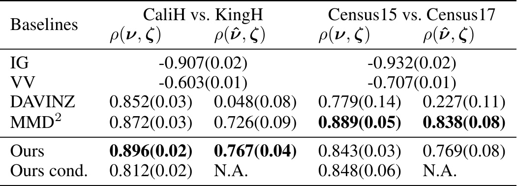
This table presents the Pearson correlation coefficients between the ranking of data sample values and the ranking of data distribution values for classification tasks. The table compares the performance of several methods, including the proposed MMD-based method (‘Ours’), against existing baselines (LAVA, DAVINZ, CS, MMD2) across various datasets (CIFAR10 vs. CIFAR100, TON vs. UGR16). Higher correlation indicates better performance of the valuation method in accurately ranking data distributions.

This table summarizes the experimental settings used in the empirical evaluation of the proposed data distribution valuation method. It lists the datasets used for classification and regression tasks, the machine learning models employed for each task, the number of vendors (n), the sample size for each vendor (mi), and the parameter controlling the heterogeneity in the Huber model (εi). The table provides a concise overview of the experimental setup, facilitating reproducibility and comparison across different settings.
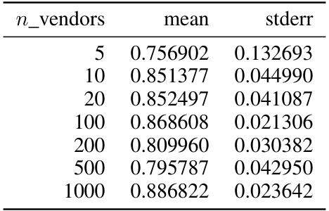
This table presents the Pearson correlation coefficients between the data sample values (obtained using various methods) and the true data distribution values for classification tasks. The Pearson correlation coefficient measures the linear association between two sets of data; a higher value indicates a stronger positive association. The table shows correlations for different numbers of vendors (n), each with a sample size (mi). The results provide insights into how well each data valuation method captures the true rankings of data distributions, based on the sample data.

This table presents the Pearson correlation coefficients between data sample values and data distribution values for a classification task using the Credit7 and Credit31 datasets. The Pearson correlation is calculated using two different methods of valuation: one which uses a validation set (ρ(ν, ζ)), and one which approximates the reference distribution (ρύ, ζ)). Several baselines (LAVA, DAVINZ, CS, MMD2, Ours, Ours cond.) are compared. The results show the correlation between the valuation of datasets and the true value of the underlying data distributions. ‘Ours cond.’ refers to the method which utilizes label information. N.A. indicates that the result is not applicable.
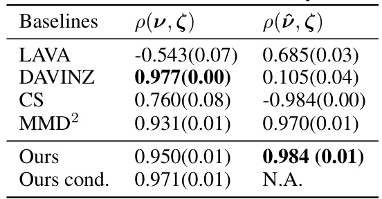
This table presents the Pearson correlation coefficients between the rankings of data sample values and the true rankings of data distributions for classification tasks. The Pearson correlation measures the strength and direction of the linear relationship between the two rankings. Higher values indicate stronger agreement between the rankings. The table compares the performance of different valuation methods: LAVA, DAVINZ, CS, MMD², Ours, and Ours cond. Ours cond. leverages label information, while Ours does not. The results are reported with standard errors over 5 independent trials and for different datasets. N.A indicates that the result is not applicable for that specific combination.
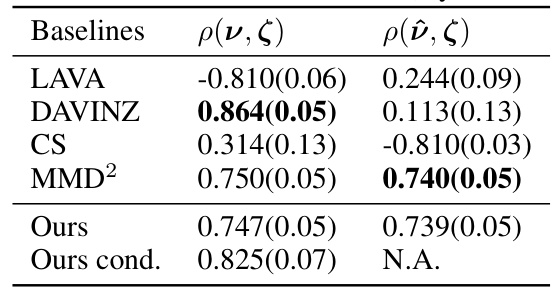
This table presents the Pearson correlation coefficients between data sample values and data distribution values for a classification task using the MNIST and FaMNIST datasets. The Pearson correlation is calculated between the rankings produced by different valuation methods and the ground truth ranking of the data distributions, to assess the accuracy of the ranking. The table shows results for various methods including LAVA, DAVINZ, CS, MMD², Ours, and Ours cond., under two conditions: when a validation set is available to help baselines and when it isn’t. Ours cond. (Ours with conditional distributions) is not applicable when a validation set isn’t available.
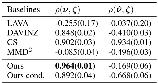
This table presents the Pearson correlation coefficients between data sample values and data distribution values for a non-Huber setting with additive Gaussian noise. It compares the performance of several baselines (LAVA, DAVINZ, CS, MMD², Ours, and Ours cond.) in ranking data distributions based on their sample datasets. The results are presented separately for when a validation set is available (ρ(ν, ζ)) and unavailable (ρ(ῦ, ζ)). The ‘Ours’ method refers to the proposed MMD-based valuation method in the paper, while ‘Ours cond.’ incorporates label information. The table highlights the relative performance of different valuation methods under this specific non-Huber data setting.
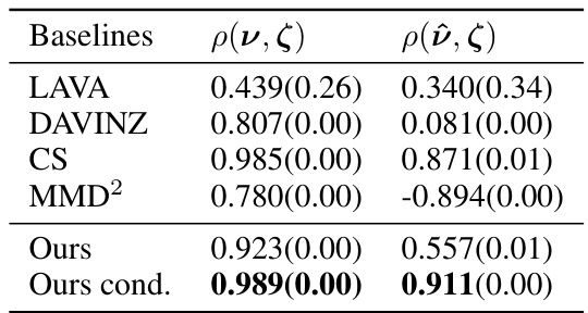
This table presents the Pearson correlation coefficients between the data sample values and the data distribution values for classification tasks. The Pearson correlation measures the linear association between the rankings of data sample values (obtained using various valuation methods) and the rankings of data distribution values (ground truth obtained from model performance on a held-out test set). Higher correlation indicates better agreement between the rankings, reflecting the effectiveness of the valuation methods in identifying the most valuable data distributions. Results are shown for multiple datasets with their corresponding classification methods and the number of vendors considered (n). The table includes results for scenarios both with and without a validation set.

This table presents the Pearson correlation coefficients between the data sample values and the data distribution values for classification tasks. The Pearson correlation measures the strength and direction of the linear relationship between the rankings of data sample values (obtained using different valuation methods) and the ground truth rankings of data distributions. Higher values indicate a stronger positive correlation, meaning the valuation method better reflects the true value of the data distributions. The results are shown for four different datasets: CIFAR10 vs. CIFAR100, TON vs. UGR16, and two cases with Dval available and unavailable, respectively.
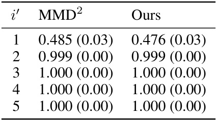
This table shows the Pearson correlation coefficients between the ground truth data values and the approximated values obtained using MMD2 and the proposed method (Ours). The ground truth values are obtained using the true distribution P* as the reference, while the approximated values are obtained using the uniform mixture Pw as the reference. The results are shown for different values of i’, which represents the index of the vendor that is mis-reporting its data. The table shows that both MMD2 and Ours have very high Pearson correlation coefficients with the ground truth values, suggesting that both methods are able to accurately capture the relationship between the true values and the approximated values. The results indicate that the proposed method is effective at identifying the mis-reporting vendor, even when the ground truth is not known.

This table shows the Pearson correlation coefficients between the ground truth data values and the approximated data values obtained using MMD2 and the proposed method for the MNIST and QEMNIST datasets with 5 vendors. The results are presented for the case where vendor i’ adds Gaussian noise to the features of their data, and the results are consistent with the ground truth results.

This table presents the Pearson correlation coefficients between the ground truth data values and the values obtained by using MMD2 and the proposed method (Ours). The ground truth values are obtained using the expected test performance. The results show high correlation (close to 1) between the ground truth and the estimated values, especially for the proposed method, suggesting that the proposed method can achieve approximate incentive compatibility.

This table presents the Pearson correlation coefficients between the ground truth data values and the approximated data values obtained using MMD2 and the proposed method (Ours), for different mis-reporting vendors (i’). The results are from an experiment to test incentive compatibility, where a vendor misreports its data by adding Gaussian noise. High correlation coefficients indicate good agreement between the true and approximated values, suggesting that incentive compatibility is approximately satisfied.
This table compares the Maximum Mean Discrepancy (MMD) method against three other methods for data distribution valuation: Kullback-Leibler (KL) divergence, Wasserstein distance (WD), and squared MMD (MMD²). The comparison considers sample and computational complexities, whether the triangle inequality holds, and compatibility with the Huber model. The MMD method is shown to be superior in several aspects, particularly its sample efficiency and theoretical guarantees.

This table compares four different distance metrics: Kullback-Leibler (KL) divergence, Wasserstein distance (WD), squared maximum mean discrepancy (MMD2), and maximum mean discrepancy (MMD). The comparison is based on their sample complexity, computational complexity, whether they satisfy the triangle inequality, and their compatibility with the Huber model for data heterogeneity. MMD is shown to have favorable properties compared to other metrics.
This table compares four different metrics (KL, WD, MMD2, and MMD) based on several criteria relevant to data distribution valuation, particularly in the context of the Huber model for data heterogeneity. These criteria include sample complexity (how much data is needed for accurate estimation), computational complexity (how much computation is needed), whether the metric satisfies the triangle inequality (a key property for theoretical analysis), and compatibility with the Huber model (whether it easily integrates into the analysis of mixture distributions). The results show that MMD excels across several of these criteria, making it particularly suitable for use in the theoretical framework of the paper.
This table compares the Maximum Mean Discrepancy (MMD) method to three other methods (Kullback-Leibler divergence, Wasserstein distance, and squared MMD) across several criteria. These criteria are sample complexity (asymptotic and finite sample), computational complexity, whether the method satisfies the triangle inequality, and whether it is compatible with the Huber model of data heterogeneity. The table highlights the advantages of MMD in terms of sample and computational efficiency, and its suitability for theoretical analysis thanks to the triangle inequality property.
This table compares the Maximum Mean Discrepancy (MMD) method to three other methods (Kullback-Leibler divergence, Wasserstein distance, and squared MMD) across several criteria. These criteria include the asymptotic and computational complexities of each method for both sample and computation, whether the method satisfies the triangle inequality, and whether the method is compatible with the Huber model for data heterogeneity.

This table compares four different divergence metrics (KL, WD, MMD2, and MMD) in terms of their sample complexity, computational complexity, whether they satisfy the triangle inequality, and their compatibility with the Huber model. The Huber model is a statistical model used in the paper to represent data heterogeneity.

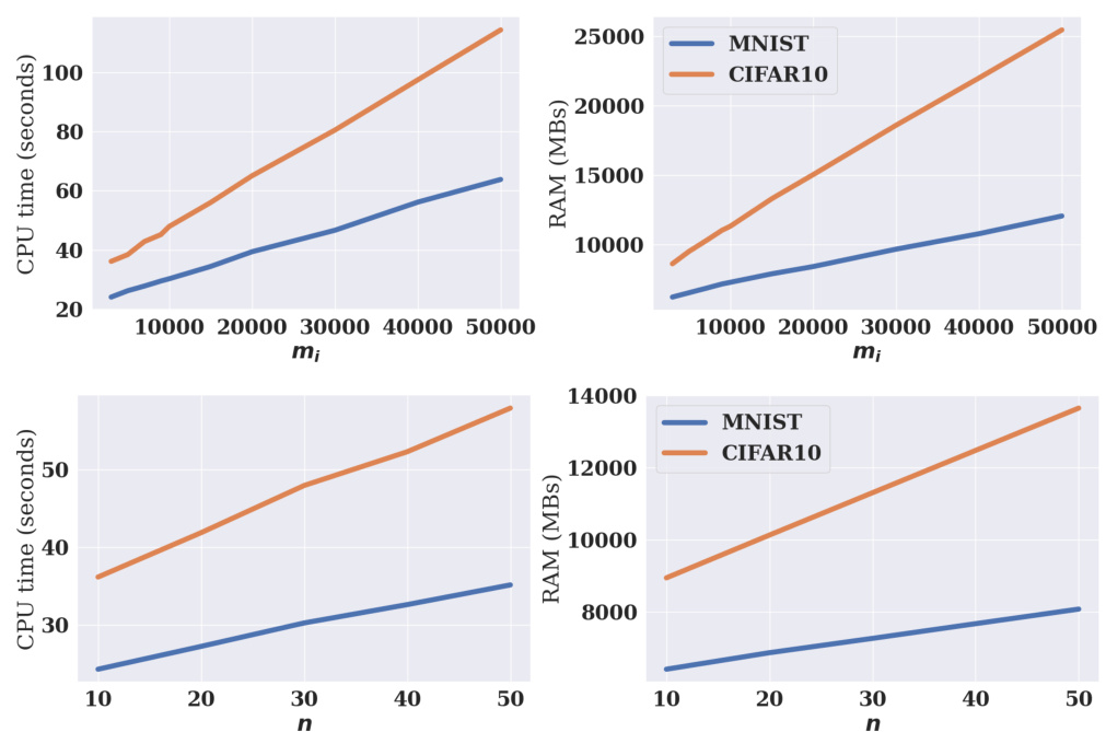
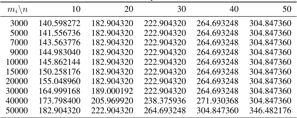
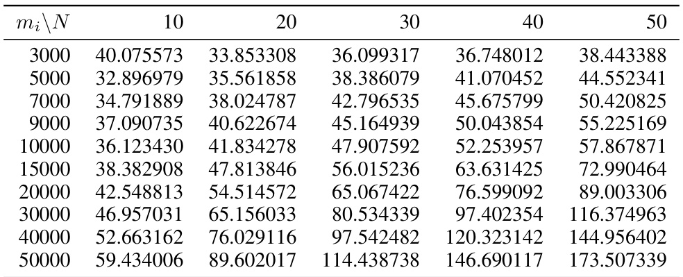
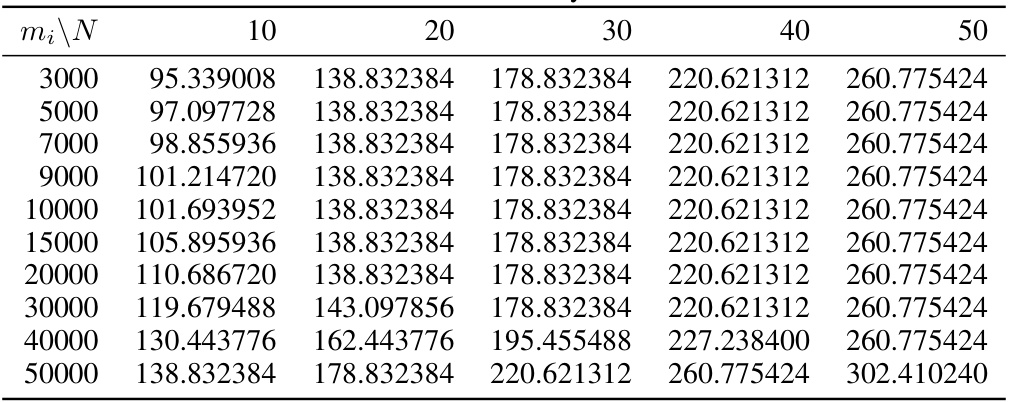
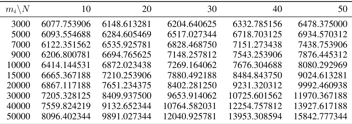
This table shows the maximum CUDA memory (in MBs), RAM (in MBs), and CPU time (in seconds) used by the DAVINZ method for different sample sizes (mi) on the MNIST dataset. The experiment uses 10 data vendors and a standard convolutional neural network. The table illustrates the scalability limitations of DAVINZ, particularly with respect to memory usage.
Full paper#
