↗ OpenReview ↗ NeurIPS Homepage ↗ Chat
TL;DR#
Time series (TS) data presents unique challenges for diffusion models, and existing methods often struggle with suboptimal performance due to the inherent non-stationarity of TS and improper noise schedules. Choosing the right noise schedule is crucial as it dictates the model’s ability to learn effectively and generate high-quality results. Poorly chosen noise schedules can lead to wasted computation and subpar outcomes.
ANT addresses this by automatically generating noise schedules tailored to the specific characteristics of each TS dataset. This is achieved by using statistics to quantify the non-stationarity of a TS dataset. ANT then selects a noise schedule that gradually reduces this non-stationarity across diffusion steps, improving learning, and ultimately leading to enhanced performance. The researchers demonstrate the effectiveness of ANT through extensive experiments, showcasing significant gains across various TS tasks.
Key Takeaways#
Why does it matter?#
This paper is important because it tackles a critical issue in time series diffusion models: suboptimal performance due to improper noise schedules. By introducing ANT, a method for automatically determining optimal noise schedules, the researchers provide a practical solution that significantly improves performance across various tasks. This work opens up new avenues for research in automated hyperparameter optimization within diffusion models, potentially impacting various fields that rely on time series analysis.
Visual Insights#
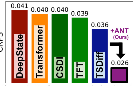
The figure shows the forecasting performance (in terms of CRPS) of various time series diffusion models on the M4 dataset. ANT (Adaptive Noise Schedule for Time Series diffusion models) achieves a significant improvement (27.8% gain) over the baseline TSDiff model by automatically selecting an appropriate noise schedule based on the dataset’s characteristics. Other models shown include DeepState, Transformer, CSDI, and TFT.

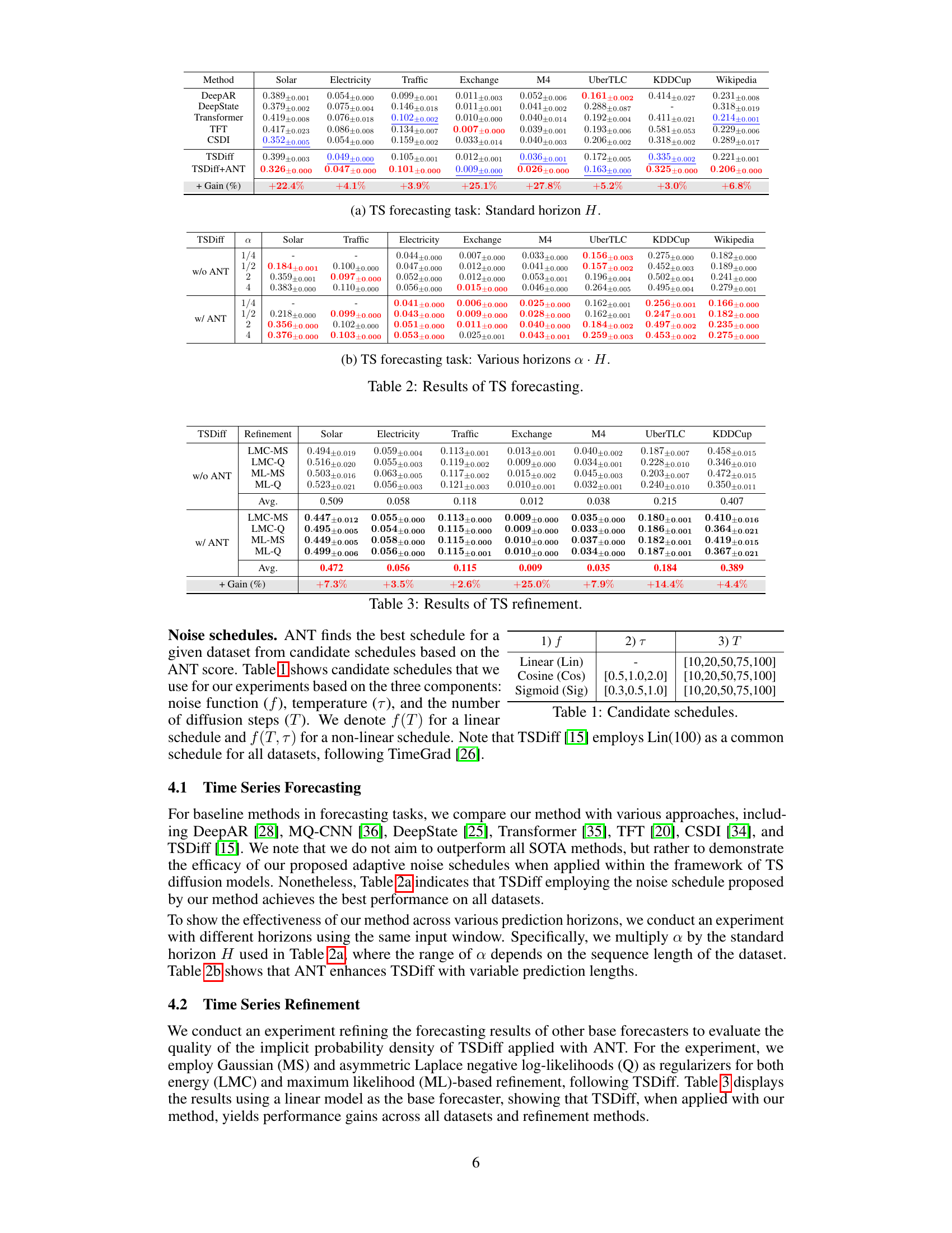
This table presents the results of time series forecasting experiments using various methods, including DeepAR, DeepState, Transformer, TFT, CSDI, TSDiff, and TSDiff+ANT (the proposed method). The results are shown for different datasets (Solar, Electricity, Traffic, Exchange, M4, UberTLC, KDDCup, and Wikipedia) and are expressed in terms of Continuous Ranked Probability Score (CRPS), a metric for evaluating probabilistic forecasts. The ‘+ Gain (%)’ column indicates the percentage improvement in CRPS achieved by TSDiff+ANT compared to the baseline TSDiff method. The table shows that TSDiff+ANT significantly outperforms TSDiff on most datasets, demonstrating the effectiveness of the proposed adaptive noise schedule.
In-depth insights#
ANT: Adaptive Noise#
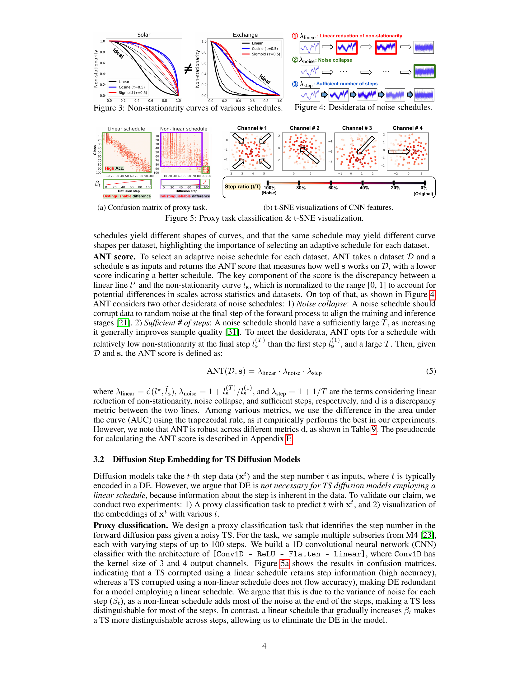
The heading “ANT: Adaptive Noise” suggests a method for adjusting noise levels in a system, likely a machine learning model, in an adaptive manner. Adaptive implies the noise adjustment isn’t static but changes dynamically based on some criteria. The “ANT” acronym, while not explained here, likely represents a specific methodology or algorithm developed by the authors. The adaptive nature points towards a system that learns and optimizes noise settings during training or operation. This approach could be beneficial in scenarios where a constant noise level is suboptimal. For instance, the model might start with higher noise levels initially to explore a wider solution space, then gradually reduce noise as it learns to focus on a more refined solution. The key advantage would be improved performance and potentially faster convergence compared to methods using fixed noise schedules. We can infer that the paper details the implementation and evaluation of this adaptive noise technique, possibly showing performance gains on various tasks.
Non-stationary TS#
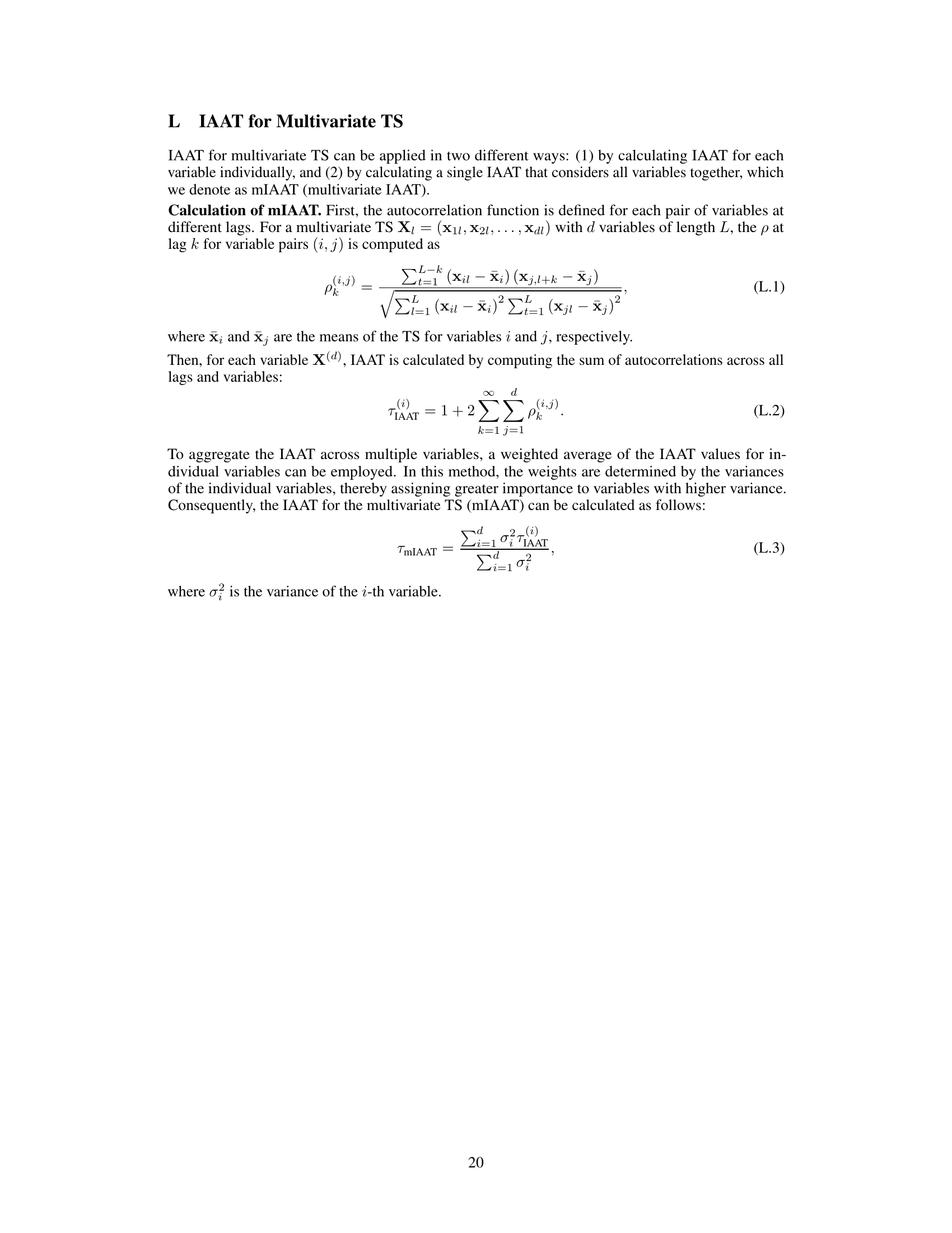
The concept of ‘Non-stationary TS’ (Time Series) is crucial to understanding the paper’s core contribution. Non-stationarity refers to the inherent characteristic of many real-world time series, where statistical properties like mean, variance, or autocorrelation change over time. The authors cleverly leverage this characteristic by recognizing that standard noise scheduling techniques often fail to account for the evolving nature of non-stationary data. They propose an adaptive noise scheduling method that implicitly understands the time series’ non-stationarity, making the diffusion process more effective and enabling better performance. Quantifying non-stationarity is a key part of their approach, using statistics like integrated autocorrelation time (IAT) and its absolute version (IAAT) to characterize the data and guide the selection of appropriate noise schedules. This thoughtful consideration of the intrinsic data properties distinguishes their method, demonstrating that addressing non-stationarity directly leads to superior diffusion model training and, consequently, superior results in time series forecasting, refinement, and generation.
Linear Schedule Use#
The concept of ‘Linear Schedule Use’ within the context of time series diffusion models is crucial for understanding the paper’s core contribution. A linear schedule, in this context, refers to how noise is gradually added (forward diffusion) or removed (reverse diffusion) during the process of training the diffusion model. The key advantage of a linear schedule is its simplicity and efficiency. It systematically reduces non-stationarity in time series data, ensuring all diffusion steps contribute equally to the training process, unlike abrupt noise introduction seen in other schedules. This linear reduction enables the model to better learn the underlying temporal dependencies. The paper highlights that employing a linear schedule makes diffusion step embedding unnecessary, simplifying model architecture and improving efficiency. While a linear schedule offers these advantages, the paper also explores the robustness of non-linear alternatives. The superior performance and robustness of non-linear schedules, particularly regarding the number of diffusion steps, is a key finding. Therefore, the choice between a linear and non-linear schedule depends on a tradeoff between simplicity and robustness to the specific characteristics of a given time series dataset.
ANT Score Robustness#
The robustness of the ANT score is crucial for its reliability and practical applicability. Robustness to various non-stationarity statistics ensures the method’s effectiveness across different datasets and their specific characteristics. The authors demonstrate this by testing the score with multiple statistics, indicating consistent performance despite variations in how non-stationarity is measured. Robustness to the choice of discrepancy metric between the ideal and actual non-stationarity curves further strengthens the ANT score’s reliability. The study’s exploration of multiple discrepancy metrics highlights the score’s resilience to different mathematical representations of curve similarity. Insensitivity to the total number of diffusion steps (T) is a significant advantage, allowing flexible application across various computational constraints. This characteristic is demonstrated by consistent results across different T values, ensuring practicality regardless of resource limitations. In essence, the multifaceted robustness checks detailed in the paper significantly enhance the ANT score’s credibility and establish its value as a reliable tool for adaptive noise schedule selection in time series diffusion models. Further investigation into the sensitivity to other hyperparameters would provide additional insights into its overall robustness.
Future Research#
The paper’s ‘Future Research’ section could explore several promising avenues. Extending ANT to other generative models beyond diffusion models is crucial. Investigating the applicability of ANT to different data modalities (images, text) would broaden its impact. Developing more sophisticated non-stationarity metrics is important to capture nuanced temporal dynamics. Currently, ANT relies on a single metric; a multi-faceted approach would improve robustness and accuracy. A deeper theoretical analysis of the relationship between noise schedule, non-stationarity, and model performance is needed. The current work provides empirical evidence, but rigorous theoretical understanding would strengthen its foundations. Investigating the impact of different noise schedule types is another avenue. While the paper explores several types, a more exhaustive study could reveal further insights. Finally, exploring different optimization strategies for finding the optimal schedule could enhance efficiency. The current method may not scale well for extremely large datasets; optimized search algorithms could address this limitation.
More visual insights#
More on figures

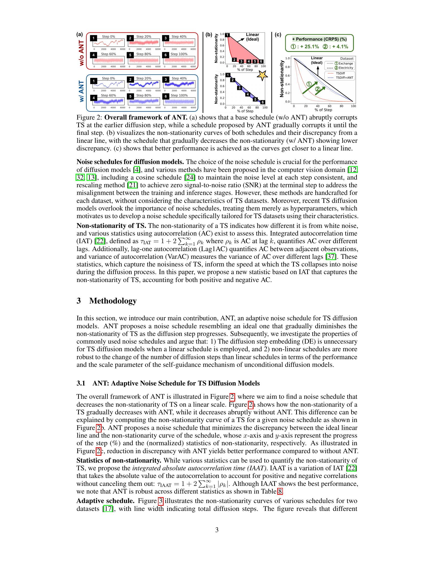
This figure demonstrates the adaptive noise schedule (ANT) proposed in the paper. Panel (a) compares the forward diffusion process of a standard noise schedule with ANT’s adaptive schedule. It highlights how ANT gradually corrupts the time series (TS) data into noise, unlike the abrupt corruption seen in standard schedules. Panel (b) shows non-stationarity curves for both schedules, plotting non-stationarity against the percentage of diffusion steps. ANT’s schedule exhibits a more linear decrease in non-stationarity, implying a smoother and more effective diffusion process. Finally, panel (c) shows a correlation between the linearity of the non-stationarity curve and the forecasting performance, indicating that schedules with a more linear non-stationarity reduction achieve better results.
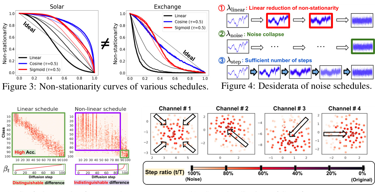
This figure illustrates the ANT framework. It demonstrates how the proposed adaptive noise schedule (ANT) gradually corrupts the time series (TS) data into random noise, unlike the abrupt corruption of a baseline schedule. The figure also shows how ANT reduces non-stationarity and improves model performance by making the non-stationarity curves closer to a linear line.

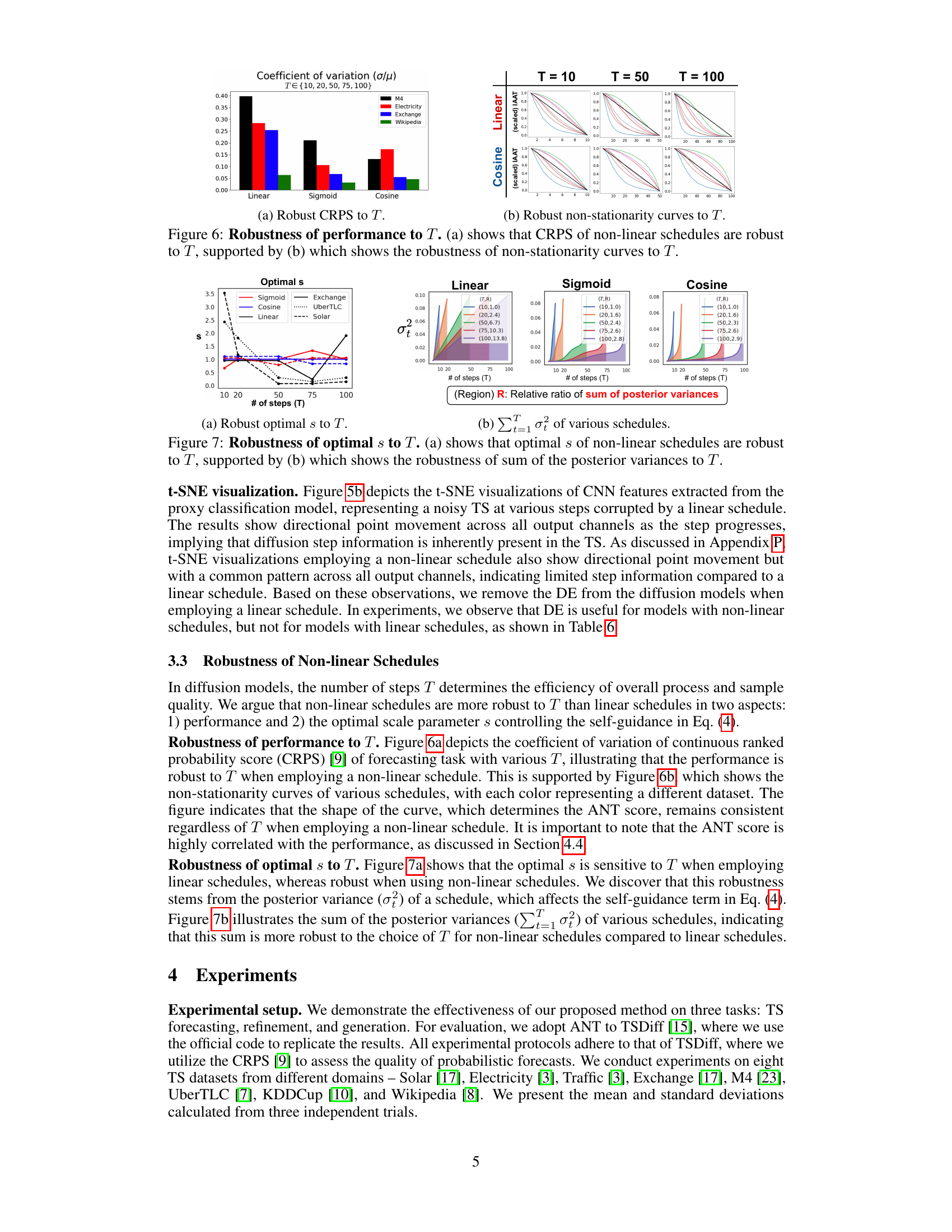
This figure demonstrates the robustness of non-linear noise schedules (cosine and sigmoid) compared to linear schedules in terms of continuous ranked probability score (CRPS) and non-stationarity curves, across different numbers of diffusion steps (T). The left panel (a) shows that the coefficient of variation of CRPS remains relatively constant for non-linear schedules as T increases, indicating stability of performance regardless of the number of diffusion steps. In contrast, linear schedules show more variability. The right panel (b) visually confirms this by showing that the shapes of the non-stationarity curves for non-linear schedules remain consistent across different T values, whereas linear schedules show a more significant change in curve shape as T varies. This suggests that non-linear schedules are less sensitive to the hyperparameter T, leading to more reliable performance.

This figure demonstrates the robustness of non-linear noise schedules to changes in the total number of diffusion steps (T). Panel (a) shows that the continuous ranked probability score (CRPS), a measure of forecasting accuracy, remains relatively stable for non-linear schedules across different values of T. In contrast, linear schedules exhibit more variability in CRPS as T changes. Panel (b) visually supports this finding by showing that the non-stationarity curves for non-linear schedules remain consistent across various T values, indicating their robustness to the choice of T.

This figure presents an ablation study on the Adaptive Noise Schedule (ANT) method. Panel (a) shows a scatter plot illustrating the relationship between ANT score and the Continuous Ranked Probability Score (CRPS), a measure of forecasting performance. A lower ANT score indicates a better-performing schedule. Panel (b) shows a bar chart visualizing the correlation between the ANT score and CRPS when using different combinations of ANT’s components (linear reduction of non-stationarity, noise collapse, and sufficient number of steps). The results demonstrate that using all three components yields the strongest correlation, highlighting the effectiveness of ANT’s comprehensive approach.
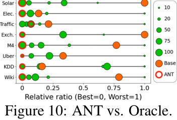
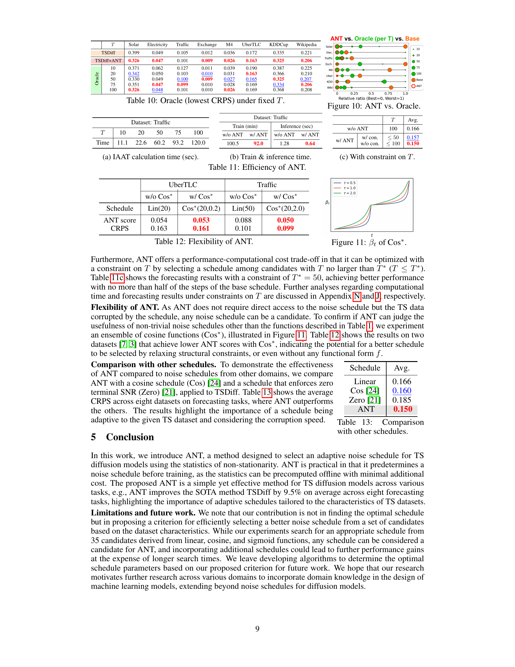
This figure visualizes the performance of ANT in selecting optimal noise schedules compared to an oracle. For each dataset (Solar, Electricity, Traffic, Exchange, M4, UberTLC, KDDCup, Wikipedia), it shows the relative ratio of the ANT score to the oracle score for different numbers of diffusion steps (T = 10, 20, 50, 75, 100). A lower relative ratio indicates better performance. The size of the circles represents the value of the CRPS (Continuous Ranked Probability Score), with larger circles representing worse performance. The red circles represent the schedules selected by ANT, while the orange circles represent the baseline schedule.

This figure illustrates the ANT framework. Panel (a) compares the forward diffusion process using a standard schedule and ANT’s adaptive schedule, highlighting how ANT gradually corrupts the time series (TS) data into noise, unlike the abrupt corruption of the standard schedule. Panel (b) shows the non-stationarity curves for both schedules and their deviation from a perfect linear decrease. The adaptive schedule from ANT exhibits a lower discrepancy. Panel (c) demonstrates that improved performance is directly related to how close the non-stationarity curve is to a linear decrease.
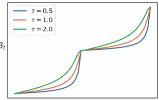
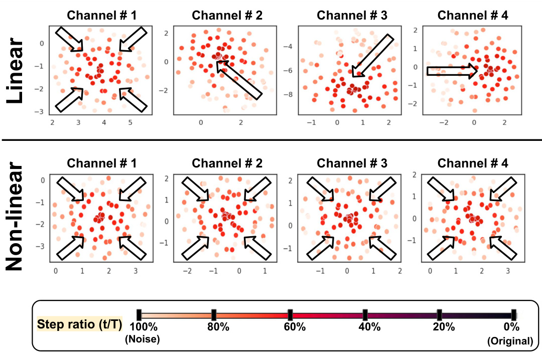
This figure shows the βt (variance of the noise) across different steps for a cosine schedule with different temperature parameters (τ). The x-axis represents the diffusion steps, and the y-axis represents the βt values. The different colored lines show the βt values for τ = 0.5, τ = 1.0, and τ = 2.0. The figure demonstrates the impact of the temperature parameter on the shape of the noise schedule, with higher temperatures leading to a more abrupt increase in noise towards the end of the diffusion process.
This figure demonstrates the ANT’s adaptive noise schedule. The leftmost panel (a) compares the forward diffusion process of TSDiff with and without ANT. While the base schedule (without ANT) abruptly corrupts the time series, ANT gradually reduces non-stationarity until it reaches random noise. The middle panel (b) visualizes this by plotting non-stationarity against the diffusion process. ANT’s approach aims to create a linear non-stationarity decrease. The rightmost panel (c) shows that better performance is related to non-stationarity curves more closely approximating a linear decrease.
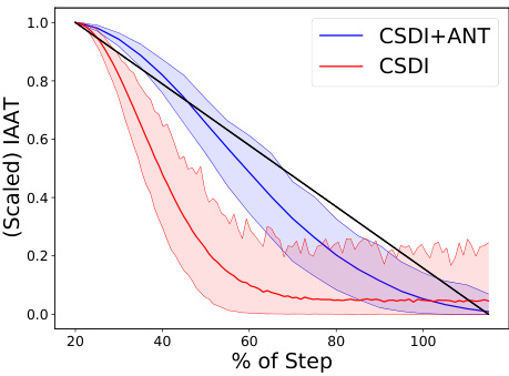
This figure visualizes the non-stationarity curves for all variables of the Solar dataset using both the base schedule and the schedule proposed by ANT. The shaded area represents the 5th and 95th percentiles. It shows that ANT’s proposed schedule more closely resembles the ideal linear line (black), indicating that ANT effectively reduces non-stationarity.

This figure demonstrates the ANT (Adaptive Noise Schedule for Time Series Diffusion Models) framework. Panel (a) compares the noise level at each step for a baseline schedule and ANT’s proposed schedule, illustrating how ANT gradually corrupts time series data into noise. Panel (b) visualizes non-stationarity through the diffusion process for both the baseline and ANT; the less deviation from a linear decrease of the non-stationarity curve the better. Panel (c) displays the correlation between the performance and discrepancy from a linear line, suggesting that smaller discrepancies mean better performance.
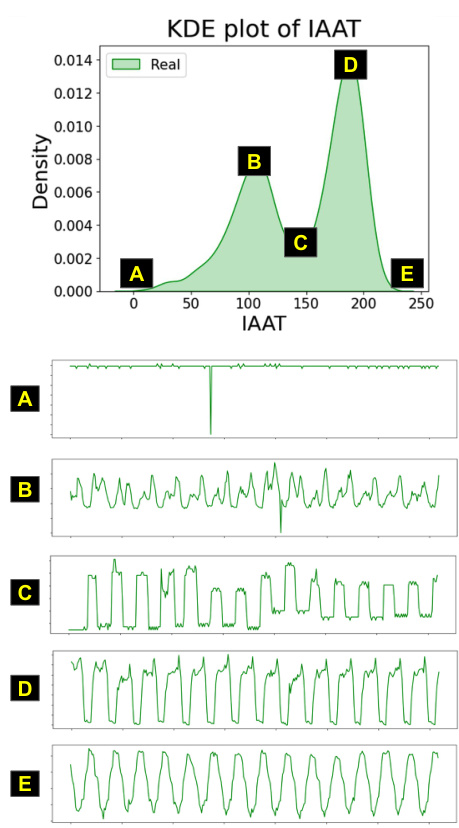
This figure visualizes the distribution of the Integrated Absolute Autocorrelation Time (IAAT) for real and generated time series data using different methods (Real, TSDiff, and TSDiff+ANT). Subfigure (a) shows histograms, (b) displays kernel density estimations, and (c) illustrates Gaussian mixture model fits. The figure helps to compare the similarity of the generated time series data distribution to that of the real data, demonstrating the effectiveness of ANT in improving the quality of generated time series data.
This figure illustrates the ANT framework. It compares the base schedule (without ANT) with the proposed ANT schedule. Panel (a) shows how the non-stationarity changes over diffusion steps for both methods, highlighting the gradual corruption in ANT versus abrupt corruption in the base schedule. Panel (b) plots non-stationarity curves against diffusion step percentage, demonstrating that ANT leads to a curve closer to linear decrease. Finally, panel (c) shows that better performance correlates with a more linear non-stationarity curve.
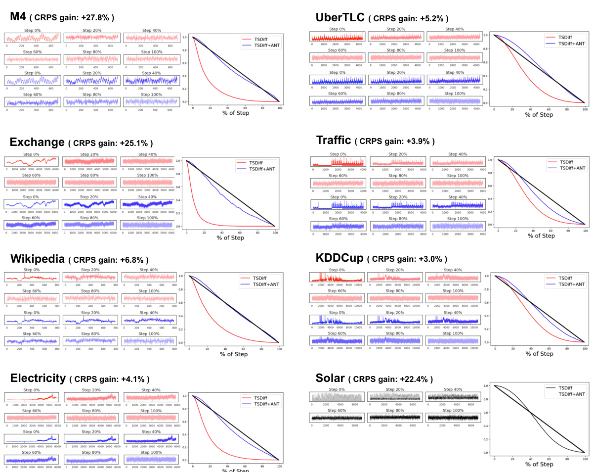
This figure demonstrates the forecasting performance improvement achieved by ANT (Adaptive Noise Schedule for Time Series diffusion models) on the M4 dataset, compared to several other time series forecasting methods. It highlights ANT’s ability to choose an appropriate noise schedule based on the dataset’s statistics, achieving a 27.8% gain in forecasting accuracy over a linear schedule using TSDiff.
More on tables

This table presents the results of time series forecasting experiments on eight different datasets using various methods. It compares the performance of the proposed ANT method (applied to TSDiff) with other state-of-the-art time series forecasting approaches, including DeepAR, DeepState, TFT, CSDI, and TSDiff without ANT. The table shows the Continuous Ranked Probability Score (CRPS) for each method on each dataset, allowing for a direct comparison of forecasting accuracy across different models and datasets.

This table presents the results of time series refinement experiments conducted using various methods (LMC-MS, LMC-Q, ML-MS, ML-Q) with and without the proposed ANT method. The results are shown for eight different datasets (Solar, Electricity, Traffic, Exchange, M4, UberTLC, KDDCup, Wikipedia). The table compares the performance of the refinement methods in terms of CRPS (Continuous Ranked Probability Score) and also shows the percentage gain achieved by using ANT. Lower CRPS values indicate better refinement performance.

This table lists the candidate noise schedules explored in the ANT experiments. It shows three different noise functions (Linear, Cosine, Sigmoid), each evaluated with varying temperature parameters (τ) and numbers of diffusion steps (T). The combinations of these parameters form the pool of candidate schedules from which ANT selects the optimal schedule for each dataset.
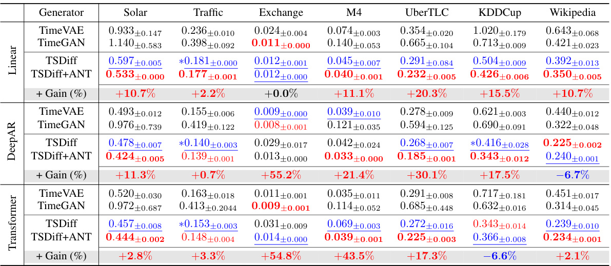
This table presents the results of time series forecasting experiments using various methods, including DeepAR, DeepState, TFT, CSDI, and TSDiff, with and without ANT. The results are shown for various datasets and prediction horizons. The ‘+ Gain (%)’ column shows the percentage improvement in performance achieved by using ANT.

This table presents the results of time series forecasting experiments conducted on eight datasets using various methods, including DeepAR, DeepState, TFT, CSDI, and TSDiff. The table compares the Continuous Ranked Probability Score (CRPS) achieved by each method across the different datasets. It highlights the performance improvement obtained by using ANT (Adaptive Noise Schedule for Time series diffusion models) with TSDiff compared to TSDiff without ANT and other baseline methods.
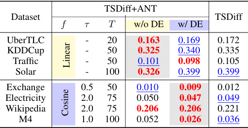
This table presents the results of time series refinement experiments. It compares the performance of TSDiff with and without ANT (Adaptive Noise Schedule) across eight different datasets and using different refinement methods (ML-MS, ML-Q, LMC-MS, LMC-Q). The ‘Gain (%) column shows the percentage improvement achieved by using ANT.

This table presents the results of an ablation study conducted to evaluate the contribution of each component of the ANT (Adaptive Noise Schedule) score in selecting an appropriate noise schedule for time series diffusion models. The ANT score comprises three components: Alinear (linear reduction of non-stationarity), Anoise (noise collapse), and Astep (sufficient number of steps). The table shows the schedules selected by ANT when using different combinations of these components, including when all three components are used or when only some are utilized. The ‘Oracle’ row indicates the best-performing schedule for each dataset, providing a benchmark for comparison.

This table demonstrates the robustness of ANT to the choice of statistics for measuring non-stationarity. It shows the average CRPS across eight datasets for forecasting tasks using ANT with various statistics (VarAC, Lag1AC, IAAT). The results indicate that ANT outperforms the model without ANT across all statistics, with IAAT showing the best performance. This is likely because IAAT considers AC at all lags, while Lag1AC and VarAC focus on single lags and variance of AC, respectively.

This table presents the Continuous Ranked Probability Score (CRPS) for various time series forecasting methods applied to eight different datasets. The methods compared include DeepAR, DeepState, TFT, CSDI, TSDiff, and TSDiff+ANT (the proposed method). The table shows the CRPS values for each method on each dataset, allowing for a comparison of performance across different models and datasets. Lower CRPS values indicate better forecasting accuracy. The ‘Gain (%) column shows the percentage improvement of TSDiff+ANT over the baseline TSDiff model for each dataset.
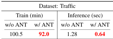
This table compares the training and inference times of TSDiff with and without ANT across eight datasets. The training time is reduced for datasets where linear schedules are selected by ANT because diffusion step embedding is eliminated. Inference time efficiency improves due to the reduced number of diffusion steps (T) used with ANT.

This table displays the inference time of the TSDiff model with different numbers of diffusion steps (T). The results show that a smaller T leads to faster inference time, with the best forecasting performance achieved at T=75. Notably, even though the base schedule uses a larger T (100), its inference time is slower and its performance worse.
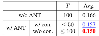
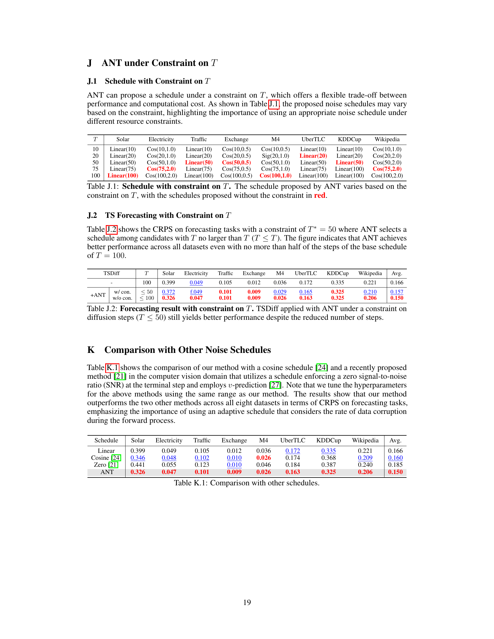
This table presents the Continuous Ranked Probability Score (CRPS) results for time series forecasting tasks, comparing models with and without the ANT method. A constraint is applied on the maximum number of diffusion steps (T). The results demonstrate that ANT, even with fewer diffusion steps, can still achieve better performance than the baseline model without ANT.
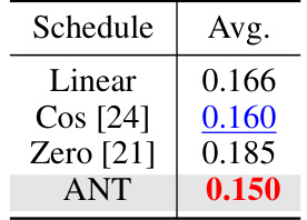
This table compares the average CRPS (Continuous Ranked Probability Score) across eight datasets for time series forecasting using three different noise schedules: Linear, Cosine [24], and Zero [21]. The results demonstrate the superior performance of the ANT method compared to existing approaches.

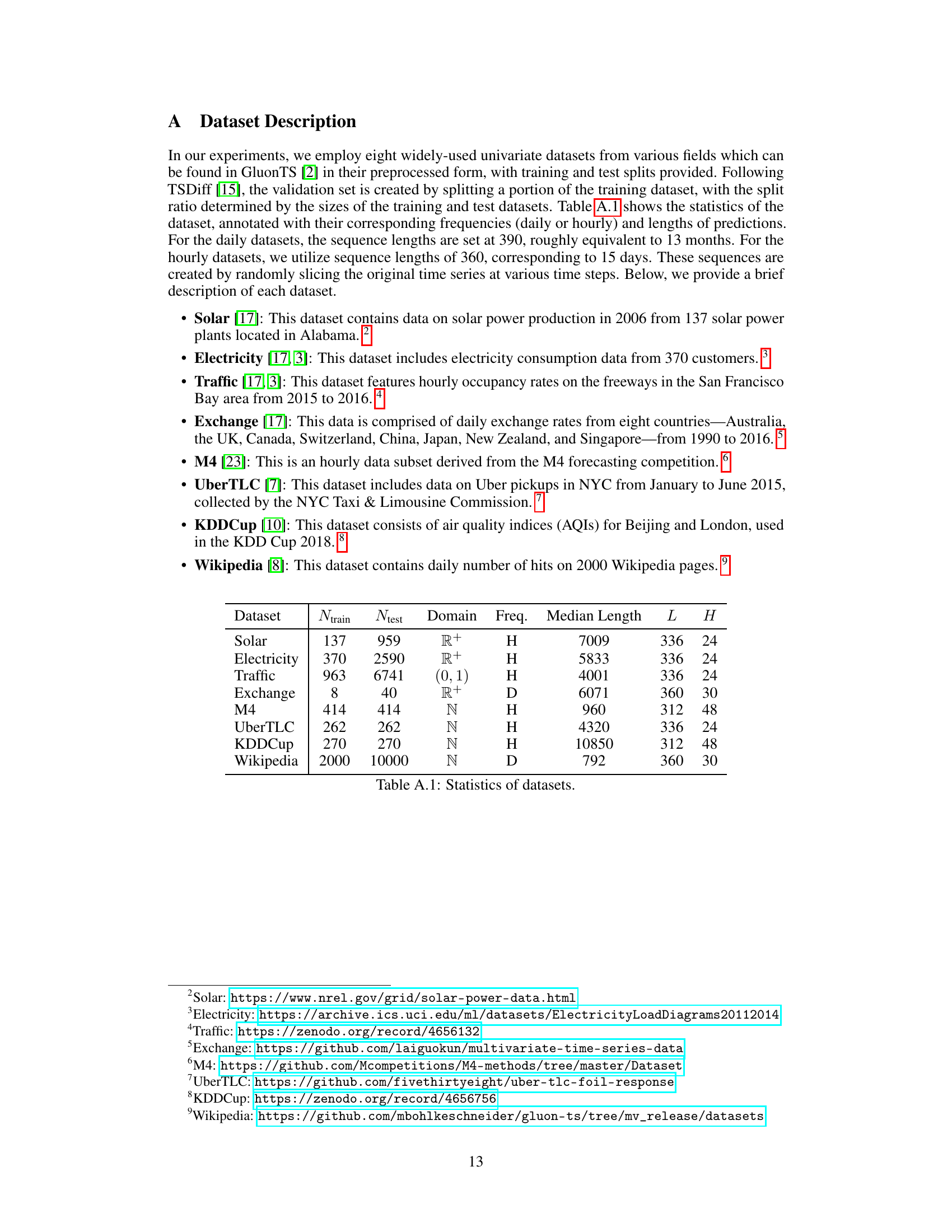
This table presents the statistics of eight datasets used in the paper’s experiments. For each dataset, it shows the number of training and testing samples (Ntrain, Ntest), the domain the data comes from, the frequency of the data (daily or hourly), the median length of the time series, and the length of the input and target windows (L, H) used in the forecasting tasks.

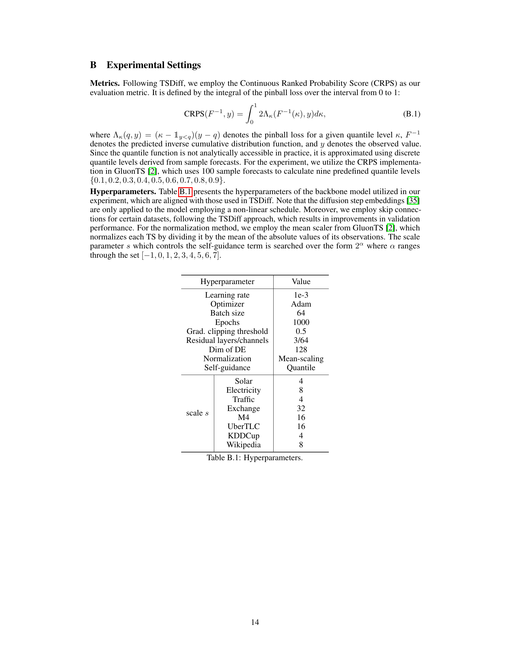
This table lists the hyperparameters used in the experiments of the paper, including the learning rate, optimizer, batch size, epochs, gradient clipping threshold, number of residual layers and channels, dimension of diffusion step embedding, normalization method, and the self-guidance scale parameter. The table also specifies the values used for each hyperparameter and provides a separate listing of the scale parameter values for each dataset used in the experiments.

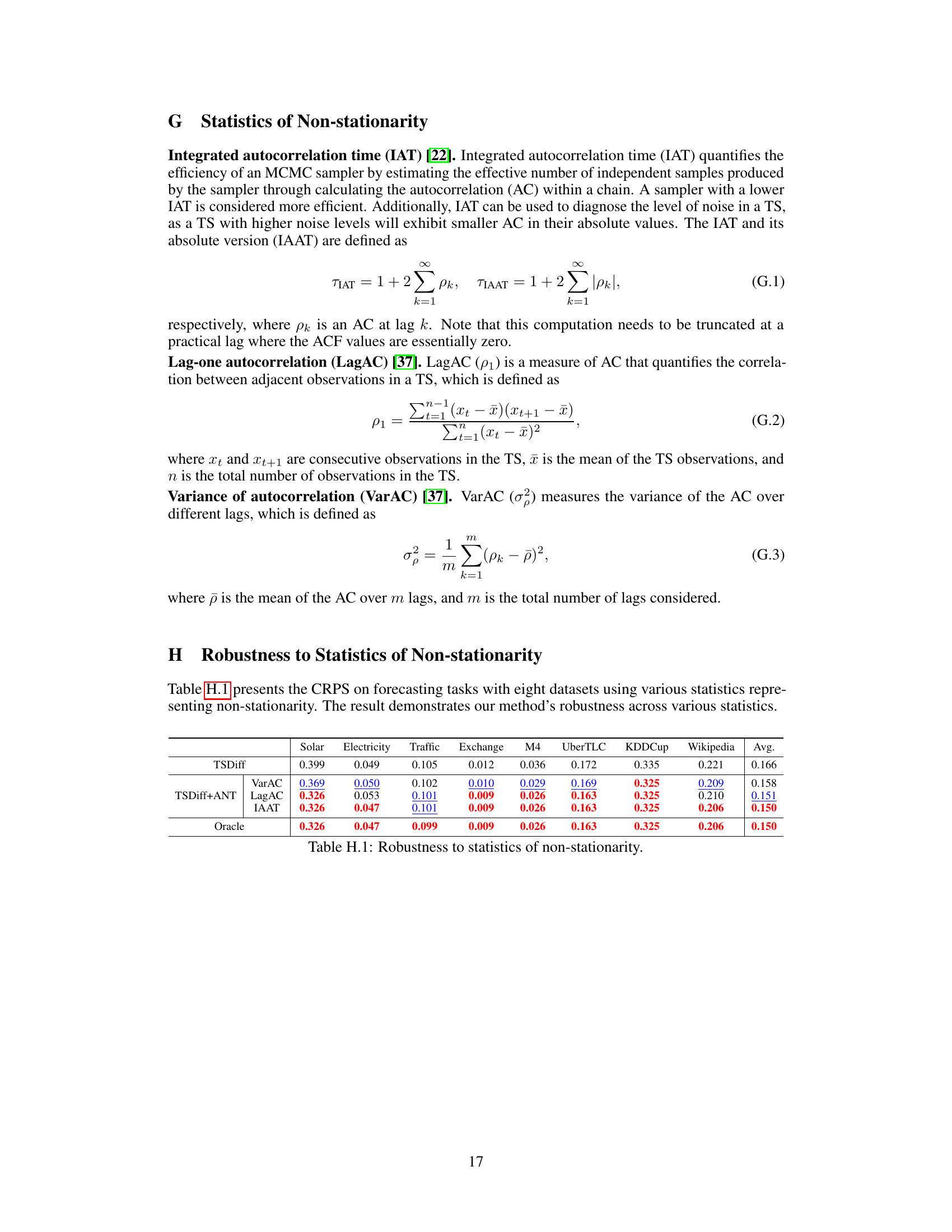
This table demonstrates the robustness of the ANT method across various statistics used to quantify non-stationarity in time series. It shows the CRPS (Continuous Ranked Probability Score) for time series forecasting across eight datasets (Solar, Electricity, Traffic, Exchange, M4, UberTLC, KDDCup, Wikipedia) using the TSDiff model without ANT and with ANT using three different non-stationarity statistics (VarAC, LagAC, IAAT). The ‘Oracle’ row indicates the best possible CRPS achievable for each dataset. The table’s purpose is to show that ANT’s performance is consistent regardless of which non-stationarity metric is used.

This table presents an ablation study on the ANT (Adaptive Noise Schedule) method. It shows the schedules selected by ANT when using different combinations of its three components: linear reduction of non-stationarity (Alinear), noise collapse (Anoise), and sufficient steps (Astep). By comparing the schedules obtained using different combinations of components with the oracle (best-performing schedule), we can understand the contribution of each component to ANT’s performance and identify the most important factor for schedule selection.

This table presents the CRPS (Continuous Ranked Probability Score) for forecasting tasks across eight datasets. The results are shown for three different statistics representing non-stationarity: VarAC (Variance of Autocorrelation), LagAC (Lag-one Autocorrelation), and IAAT (Integrated Absolute Autocorrelation Time). The table compares the performance of the baseline TSDiff model and the proposed TSDiff+ANT method. The ‘Oracle’ row indicates the lowest CRPS achieved among all candidate schedules for each dataset. The results demonstrate the robustness of the ANT method across various statistics of non-stationarity, as it consistently outperforms the baseline model, regardless of the chosen statistic. The IAAT statistic appears to provide the best performance in most cases.

This table presents the noise schedules proposed by the ANT algorithm under various constraints on the total number of diffusion steps (T). The schedules are shown for different datasets (Solar, Electricity, Traffic, Exchange, M4, UberTLC, KDDCup, Wikipedia) and for different values of T (10, 20, 50, 75, 100). The schedules proposed without any constraints on T are highlighted in red. This demonstrates how ANT adapts the schedule based on the dataset and resource limitations.

This table presents the results of time series forecasting experiments using various methods. The methods compared are DeepAR, DeepState, TFT, CSDI, TSDiff, and TSDiff+ANT (the proposed method). The table shows the Continuous Ranked Probability Score (CRPS) for each method on eight different datasets (Solar, Electricity, Traffic, Exchange, M4, UberTLC, KDDCup, and Wikipedia). A lower CRPS indicates better forecasting performance. The ‘Gain (%) ’ column shows the percentage improvement of TSDiff+ANT over TSDiff. The table is organized to showcase the performance improvements achieved using the ANT (Adaptive Noise Schedule) method across multiple datasets.

This table compares the performance of ANT’s adaptive noise schedule selection method against two other noise schedules commonly used in computer vision: a cosine schedule and a zero-signal-to-noise-ratio schedule. The results show ANT outperforms both on average CRPS across eight time series forecasting datasets.
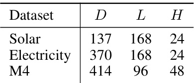
This table shows the number of variables (D), the length of the input window (L), and the length of the target window (H) for the three datasets used in the multivariate time series forecasting experiments: Solar, Electricity, and M4. The values provided are used to set up the forecasting experiments.
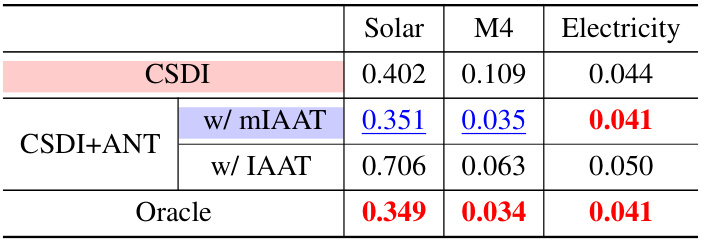
This table presents the results of time series forecasting experiments using the CSDI model with and without the ANT method. The ANT method is applied using two different strategies: one with a single noise schedule for all variables (mIAAT), and one with a variable-specific noise schedule (IAAT). The table shows the CRPS (Continuous Ranked Probability Score) achieved on three datasets (Solar, M4, and Electricity). The ‘Oracle’ row indicates the best performance achieved by any schedule on each dataset. The results demonstrate that using ANT with mIAAT improves performance.

This table displays the inference time of the TSDiff model with different numbers of diffusion steps (T). The inference time is measured in seconds, and the CRPS (Continuous Ranked Probability Score) is also provided to show how the model performance changes with the number of steps. The table highlights that a smaller number of steps can achieve better performance (lower CRPS) than a larger number of steps, demonstrating the potential efficiency gains of the proposed method (ANT).

This table compares the training and inference times of TSDiff with and without the application of ANT across eight datasets. It shows that training time is reduced for datasets where linear schedules are selected from ANT because diffusion step embedding is eliminated. The inference time efficiency gains are also shown, highlighting significant improvements in some cases due to the reduced number of diffusion steps (T).

This table presents the results of fitting Gaussian distributions to the IAATs of real and generated time series data using the TSDiff model with and without the ANT method. It displays modality, parameters (mean and variance) and the ratio of the data points assigned to each modality for both real TS and TS generated by TSDiff. The results show that real TS exhibits a multimodal distribution, whereas TSDiff without ANT captures only one modality. TSDiff with ANT captures both modalities.

This table presents the Continuous Ranked Probability Score (CRPS) and Jensen-Shannon divergence (JSD) values for the real electricity dataset and the time series generated using TSDiff with and without ANT, evaluated using three different downstream forecasters: Linear, DeepAR, and Transformer. The CRPS measures the accuracy of probabilistic forecasts, while the JSD quantifies the similarity between the probability distributions of real and generated time series in terms of their IAAT (Integrated Absolute Autocorrelation Time). Lower CRPS and JSD values indicate better performance.
Full paper#


