↗ OpenReview ↗ NeurIPS Homepage ↗ Chat
TL;DR#
Graph classification, crucial across numerous domains, faces challenges in efficiently quantifying graph similarity and representing graphs as vectors. Existing methods, like those employing graph kernels or graph neural networks (GNNs), often suffer from high computational costs, manual feature engineering (kernels), or information loss from global pooling (GNNs). These limitations hinder scalability and accuracy, particularly with large graph datasets.
This paper introduces Graph Reference Distribution Learning (GRDL), a novel and efficient graph classification method. GRDL addresses the limitations of existing approaches by directly classifying node embeddings as distributions, bypassing the need for global pooling operations and thus retaining valuable structural information. The method leverages maximum mean discrepancy (MMD) to compare graph distributions with learned reference distributions, leading to high accuracy. Importantly, the paper provides a theoretical analysis of GRDL, deriving generalization error bounds and demonstrating its superior generalization ability compared to GNNs with global pooling. Experimental results showcase GRDL’s exceptional efficiency, achieving at least a 10-fold speed improvement over state-of-the-art methods while maintaining high accuracy.
Key Takeaways#
Why does it matter?#
This paper is highly significant for researchers working on graph classification due to its novel approach and substantial improvements over existing methods. GRDL’s speed and accuracy are game-changing, particularly for large-scale datasets, while its theoretical foundation adds crucial rigor and direction to future research. It opens new avenues for developing efficient and accurate graph classification models, which have broad applications across multiple fields.
Visual Insights#
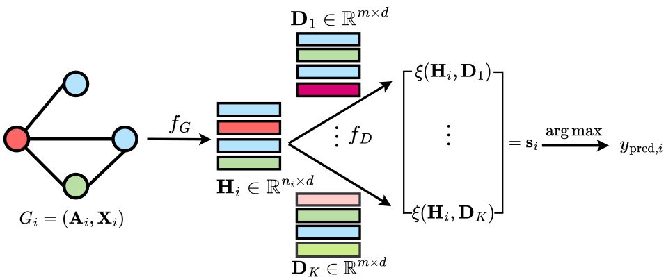
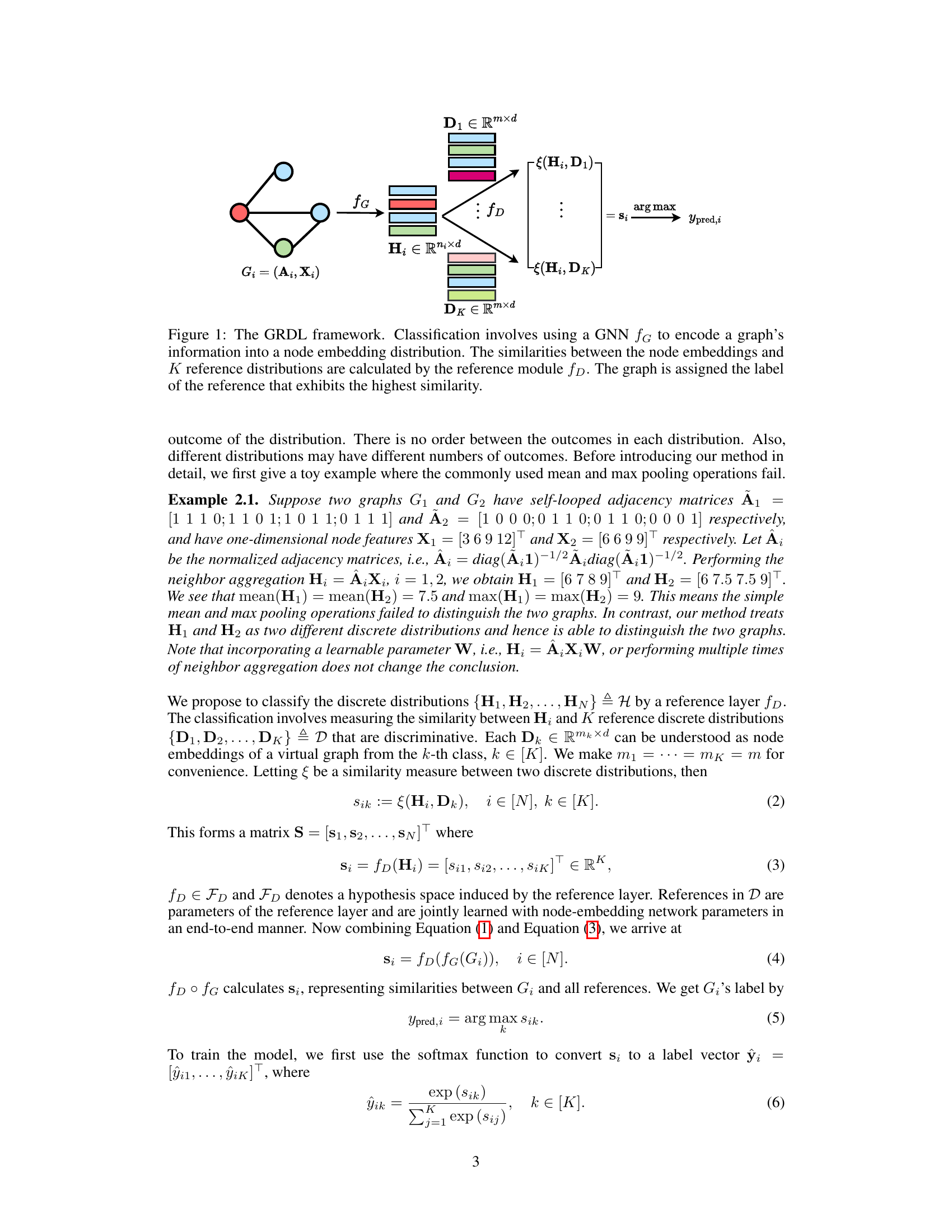
The figure illustrates the Graph Reference Distribution Learning (GRDL) framework. A graph G is first encoded by a Graph Neural Network (GNN) into a node embedding matrix H. This matrix is treated as a discrete distribution. Then, a reference module fD compares this distribution with K learned reference distributions (D1…Dk), one for each class. The graph is classified into the class of the reference distribution that has the highest similarity to the graph’s embedding distribution.
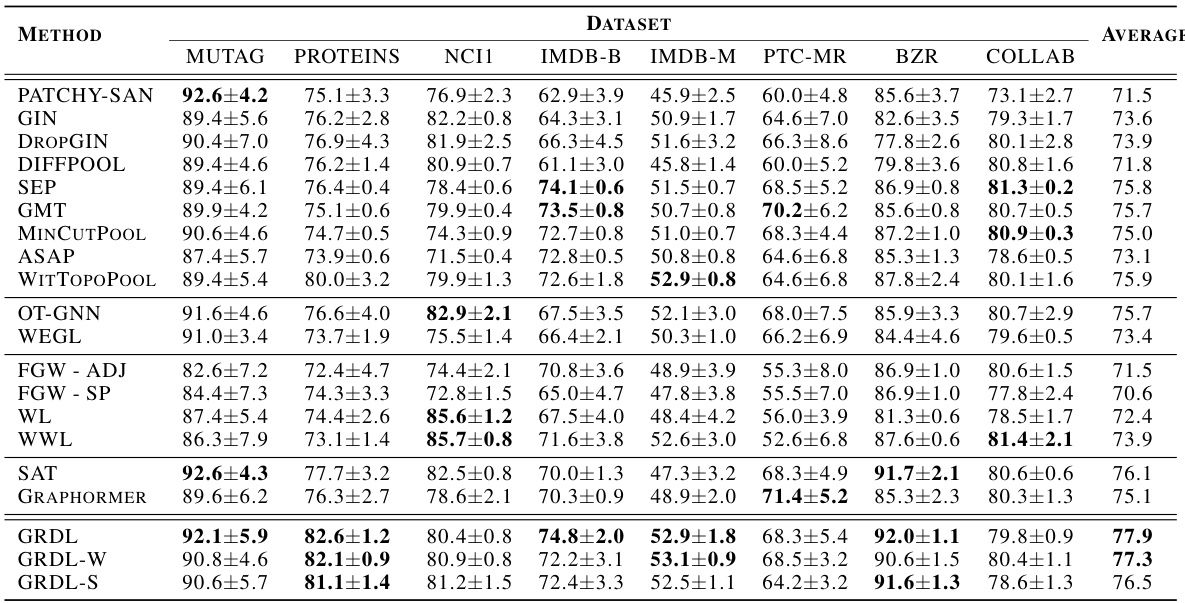
This table presents the classification accuracy results for several graph classification methods across eight benchmark datasets. The accuracy is expressed as a percentage and averaged across multiple runs. The top three methods, as determined by the average accuracy across all datasets, are highlighted in bold. The datasets encompass various domains and scales, providing a comprehensive evaluation of the different models.
In-depth insights#
RefDist Learning#
RefDist Learning, a novel approach to graph classification, tackles the challenge of representing graph structures effectively. It deviates from traditional methods by directly classifying node embeddings as discrete distributions, avoiding the information loss associated with global pooling operations. The core of the method involves calculating the similarity between a graph’s node embedding distribution and a set of adaptively learned reference distributions, each representing a different class. This framework leverages the Maximum Mean Discrepancy (MMD) to measure the distance between distributions, resulting in an efficient and accurate classification process. The theoretical analysis, providing generalization error bounds, offers valuable insights into the model’s performance and generalization capabilities, highlighting its superior generalization ability compared to GNNs with global pooling. The empirical results on various datasets demonstrate RefDist Learning’s significant efficiency and accuracy advantages over state-of-the-art competitors, offering a promising new direction for graph classification tasks.
GRDL: Theory#
The theoretical analysis of GRDL is a crucial aspect of the paper, providing a strong foundation for understanding its performance and generalization capabilities. The authors derive generalization error bounds for GRDL, a novel achievement since existing theories don’t directly apply to its unique architecture. This theoretical framework is not only valuable for understanding the model but also for guiding practical choices of hyperparameters. The derived bounds reveal the relationships between model performance and factors like network architecture, size and number of reference distributions, and properties of the input graphs. This rigorous theoretical analysis is especially important given the novelty of GRDL, making it a substantial contribution beyond empirical evaluation. The theoretical analysis also substantiates the claim that GRDL outperforms GNNs with global pooling operations, demonstrating a superior generalization ability. The theoretical insights provide valuable guidance for model design and optimization, ensuring the efficient and accurate classification of graphs across various applications.
GRDL: Practice#
The heading ‘GRDL: Practice’ suggests a focus on the practical application and implementation of the Graph Reference Distribution Learning (GRDL) method. This section would likely delve into the specifics of GRDL’s usage, including its algorithmic implementation, detailing the training process, network architecture, and hyperparameter choices. It would also cover experimental evaluations, presenting results across various benchmark datasets, comparing its performance against state-of-the-art methods. Crucially, a ‘Practice’ section should address computational efficiency and scalability, highlighting GRDL’s speed and memory usage, especially for large-scale datasets. The discussion would also likely cover practical considerations, such as the impact of parameter choices on performance and potential limitations of the approach in certain scenarios. Finally, it might include details on the accessibility and reproducibility of the work, such as code availability and instructions for implementation. Overall, the goal is to demonstrate the practicality and usability of GRDL for real-world graph classification tasks, beyond theoretical analysis.
Benchmark Results#
A dedicated ‘Benchmark Results’ section in a research paper would ideally present a thorough comparison of the proposed method against existing state-of-the-art techniques. This would involve selecting relevant and diverse benchmark datasets, ensuring fair evaluation metrics are employed, and presenting the results clearly and comprehensively. Key aspects to consider would be the statistical significance of the results, including error bars and p-values, and a discussion of the practical implications of any performance differences. The analysis should go beyond simple accuracy scores, delving into factors influencing performance, such as dataset characteristics or computational efficiency. Visualizations, such as bar charts or tables, are crucial for effective communication. A strong ‘Benchmark Results’ section ultimately provides convincing evidence of the proposed method’s effectiveness and advances the overall contribution of the research paper.
Future Works#
Future research directions stemming from this work could explore several promising avenues. Extending GRDL to handle dynamic graphs is crucial, as many real-world applications involve graphs that evolve over time. Adapting the model to incorporate temporal information and handle node/edge additions/deletions would greatly broaden its applicability. Investigating different similarity measures beyond MMD is another key area. Exploring other distance metrics, such as Wasserstein distance, while considering computational efficiency, could potentially improve classification accuracy or robustness. The theoretical analysis of GRDL could be further extended by developing tighter generalization bounds and examining the impact of specific graph properties (e.g., sparsity, degree distribution) on the model’s performance. Finally, applying GRDL to other graph-level tasks is important to assess its generalizability. Evaluating its effectiveness on problems like graph regression, clustering, or anomaly detection would demonstrate its versatility and potential.
More visual insights#
More on figures

This figure compares the average training time per epoch of the proposed GRDL model against two other models that utilize optimal transport distances: OT-GNN and TFGW. The bar chart visually represents the training time for each model across multiple graph datasets. The key takeaway is that GRDL demonstrates significantly faster training times, approximately 10 times faster than both OT-GNN and TFGW. This highlights the efficiency advantage of the GRDL approach.

This figure visualizes the results of applying t-SNE dimensionality reduction to the node embeddings generated by the GRDL model for the MUTAG dataset. The plot shows the distribution of graph node embeddings in a 3D space, where each point represents a graph. The two classes of graphs are shown in light blue and orange. Two squares represent the learned reference distributions, one for each class. The proximity of graph embeddings to the reference distributions indicates how well GRDL classifies those graphs. The clustering of the graphs around their respective reference distributions indicates that GRDL is effectively separating the two classes in the MUTAG dataset.
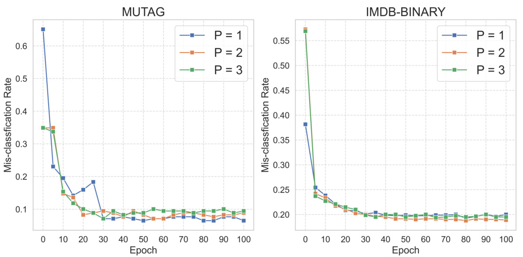
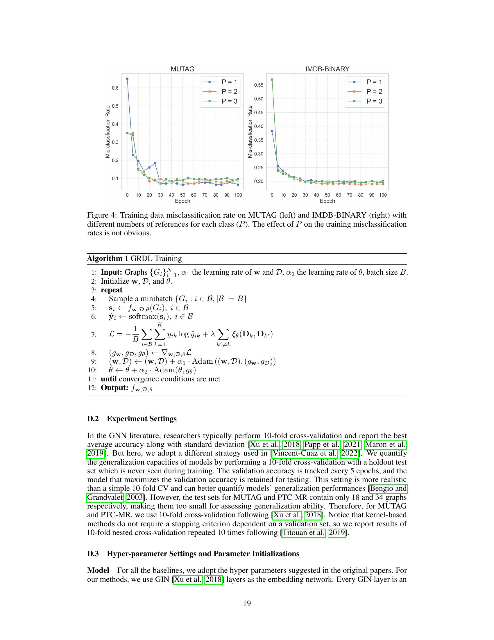
This figure shows the training misclassification rate for two datasets, MUTAG and IMDB-BINARY, while varying the number of reference distributions (P) for each class. The plots demonstrate the training misclassification rate across 100 epochs for three different values of P: 1, 2, and 3. The results show that the impact of changing P on the training misclassification rate is minimal. This observation supports a conclusion made in the paper that using a single reference distribution per class (P=1) is optimal for the GRDL model.

This figure shows the average training time per epoch for three different graph classification methods: GRDL, OT-GNN, and TFGW. The results demonstrate that GRDL is significantly faster than both OT-GNN and TFGW, achieving a speedup of at least 10 times. This highlights one of the key advantages of GRDL: its efficiency in training. The figure supports the claim made by the authors regarding GRDL’s superior efficiency compared to other state-of-the-art methods.

This figure displays the misclassification rate achieved by the GRDL model on the MUTAG and PROTEINS datasets when varying the size (m) of the reference distributions. The plots show that selecting a moderate size for the reference distributions leads to the best classification performance, avoiding both overly simplistic and overly complex representations.
More on tables
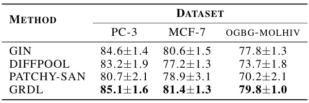
This table presents the AUC-ROC (Area Under the Receiver Operating Characteristic Curve) scores achieved by four different graph neural network models on three large, imbalanced datasets: PC-3, MCF-7, and OGBG-MOLHIV. The AUC-ROC is a common metric for evaluating the performance of binary classification models, particularly useful when dealing with imbalanced datasets. The models compared include GIN, Diffpool, Patchy-SAN, and the authors’ proposed GRDL method. The best performing model for each dataset is highlighted in bold.

This table compares the training time per epoch of GRDL with two state-of-the-art pooling methods, Wit-TopoPool and MSGNN, across eight real-world datasets and three synthetic datasets (SYN-100, SYN-300, SYN-500). The synthetic datasets vary in the number of nodes per graph (100, 300, and 500) to assess scalability. Empty cells indicate training times exceeding 200 seconds, highlighting the efficiency of GRDL. The table demonstrates that GRDL consistently exhibits faster training times compared to both Wit-TopoPool and MSGNN.

This table presents the classification accuracy results for various graph classification methods on eight benchmark datasets. The accuracy is represented as a percentage, averaged over multiple runs. The top three methods are highlighted in bold for each dataset, allowing for easy comparison of model performance across different datasets.
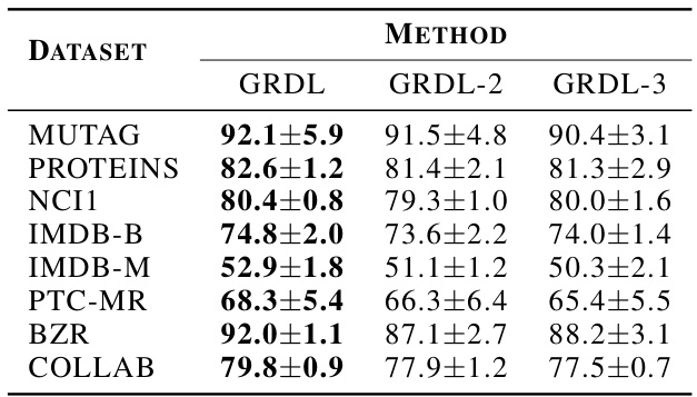
This table presents the classification accuracy results for various graph classification methods across eight benchmark datasets. The accuracy is expressed as a percentage, and the results are averaged across multiple runs, with standard deviations indicated. The top three methods with the highest average accuracy for each dataset are highlighted in bold. The datasets cover diverse domains such as bioinformatics and social networks, offering a comprehensive evaluation of the methods.

This table presents the classification accuracy results for various graph classification methods across eleven benchmark datasets. Each dataset’s accuracy is presented as a mean ± standard deviation, calculated across multiple trials. The top three performing methods for each dataset are highlighted in bold to quickly identify the best-performing algorithms.

This table presents the classification accuracy results for various graph classification methods across eight benchmark datasets and three large-scale imbalanced datasets. The accuracy is presented as an average with standard deviation across multiple runs of 10-fold cross validation. The top three performing methods for each dataset are highlighted in bold.

This table presents the classification accuracy results for several graph classification methods across eight benchmark datasets. The accuracy is reported as a percentage with standard deviation, and the top three performing methods are highlighted in bold for each dataset. The average accuracy across all datasets is also provided for each method.
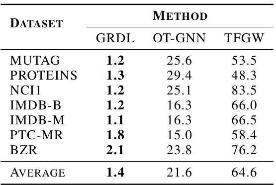
This table presents the average prediction time, measured in milliseconds, for different graph classification methods (GRDL, OT-GNN, and TFGW) across eight benchmark datasets. It shows the speed of prediction for each model, indicating the computational efficiency. The values reflect the average time taken to predict the class label of a single graph.

This table presents the classification accuracy results for various graph classification methods across eight benchmark datasets. The accuracy is reported as an average over multiple runs with standard deviation. The top three methods in terms of average accuracy are highlighted in bold for each dataset, allowing for easy comparison between the different methods.
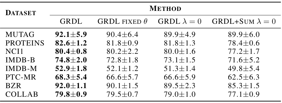
This table presents the classification accuracy results for various graph classification methods on eight benchmark datasets. The accuracy is expressed as a percentage and represents the average performance across multiple trials, with standard deviation implied by the ± notation. Bold text highlights the top three performing methods for each dataset, providing a clear comparison of the different approaches. The datasets encompass various domains, offering a robust evaluation of the models’ generalization capabilities.

This table presents the classification accuracy results for several graph classification methods across eight benchmark datasets and three large-scale imbalanced datasets. Each dataset’s results are given as mean ± standard deviation of accuracy for each method. The top three methods are highlighted in boldface for each dataset, indicating their superior performance. The table provides a comprehensive comparison of various methods and allows for the assessment of the relative performance of each algorithm on different graph structures.

This table presents the classification accuracy of various graph classification methods on eight benchmark datasets. The accuracy is expressed as a percentage and represents the average performance across multiple trials. The top three performing methods for each dataset are highlighted in bold to emphasize the relative performance of different approaches. The average accuracy across all datasets is also provided for each method.
Full paper#
