↗ OpenReview ↗ NeurIPS Homepage ↗ Chat
TL;DR#
Current novel view synthesis methods often struggle with generating efficient and generalizable 3D scene representations. Many methods directly combine pixel-aligned Gaussians from multiple views, leading to artifacts and increased memory costs. They also fail to fully capture the relationships between Gaussians from different images, limiting their generalizability and efficiency.
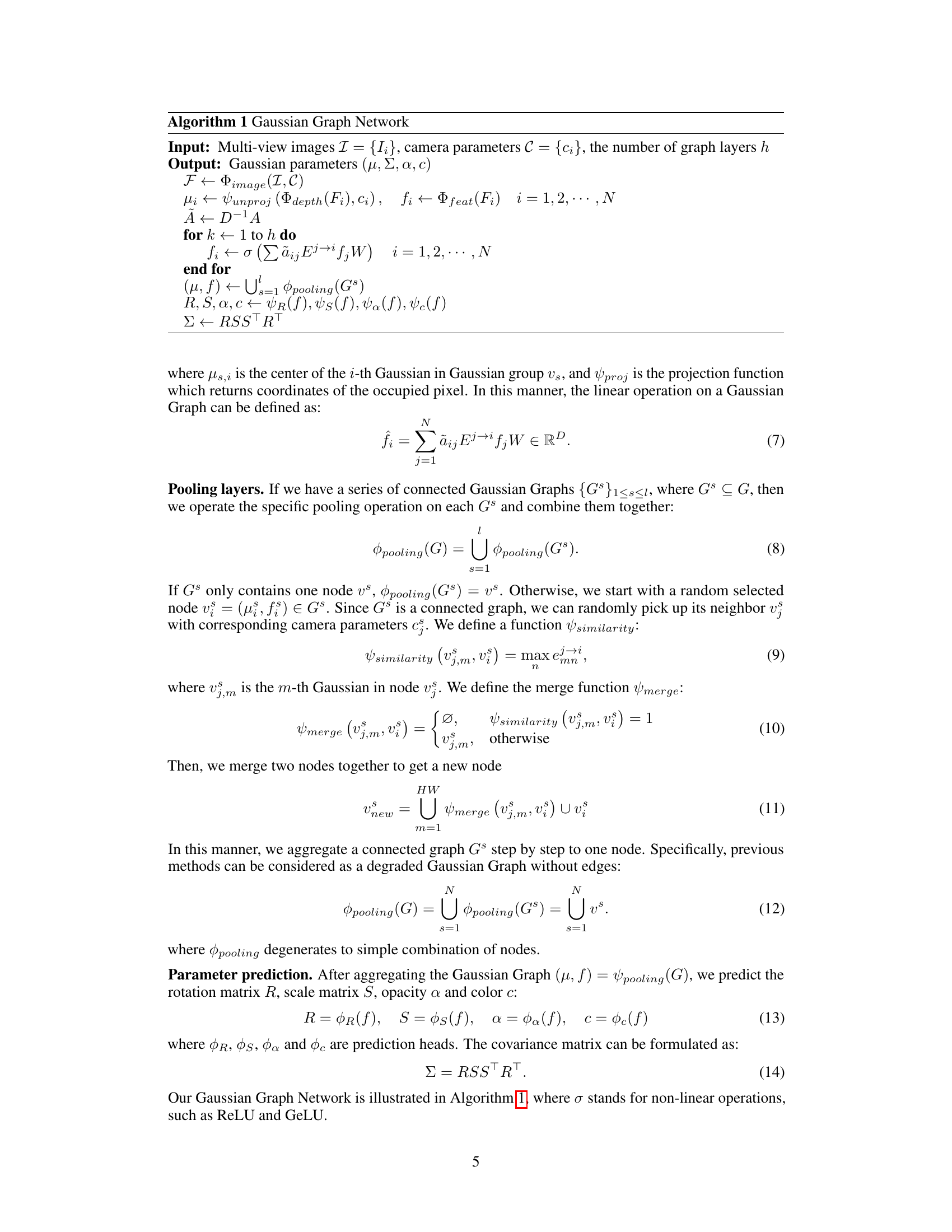
The paper introduces the Gaussian Graph Network (GGN) to address these issues. GGN constructs Gaussian Graphs to model the relationships between Gaussian groups, enabling message passing and feature fusion at the Gaussian level. A Gaussian pooling layer efficiently aggregates information from different groups. Experiments show that GGN significantly outperforms existing methods in terms of rendering quality and efficiency, requiring fewer Gaussians and delivering higher rendering speeds, particularly with increasing numbers of input views. The model demonstrates strong generalization across various datasets.
Key Takeaways#
Why does it matter?#
This paper is significant as it presents Gaussian Graph Network (GGN), a novel approach that improves the efficiency and generalizability of 3D Gaussian representations for novel view synthesis. This addresses a key challenge in computer vision and graphics by achieving higher rendering quality with fewer Gaussian representations and faster rendering speeds compared to existing methods. The method’s ability to leverage information across multiple views opens avenues for further research into more efficient and robust 3D scene representation techniques.
Visual Insights#
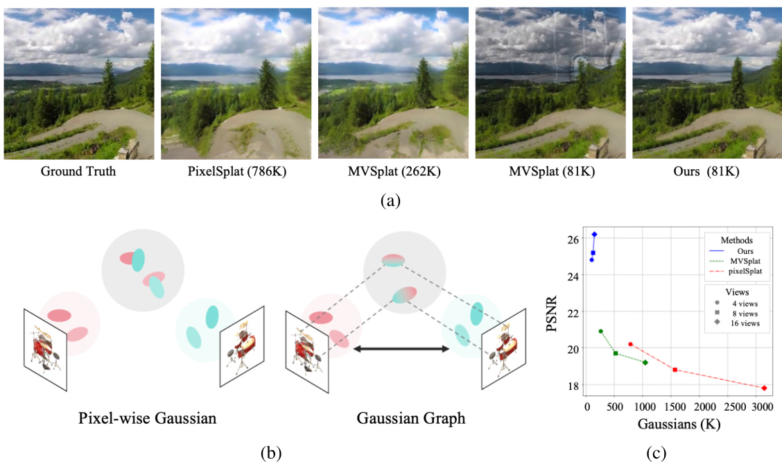
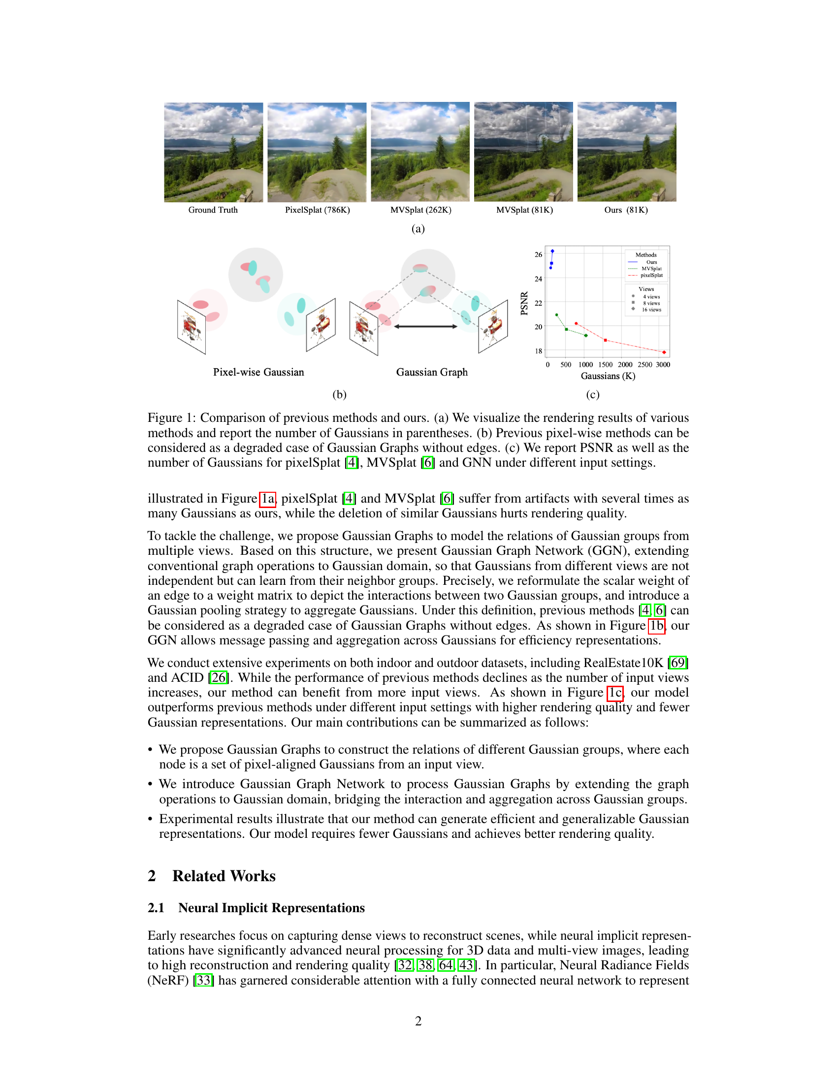
This figure compares the novel view synthesis results of the proposed Gaussian Graph Network (GGN) with those of existing methods, namely PixelSplat and MVSplat. Subfigure (a) shows a qualitative comparison of the rendered images, highlighting the improved visual quality of GGN despite using significantly fewer Gaussians. Subfigure (b) illustrates the conceptual difference between the pixel-wise Gaussian approach of previous methods and the Gaussian Graph representation used in GGN. Subfigure (c) presents a quantitative comparison in terms of Peak Signal-to-Noise Ratio (PSNR) and the number of Gaussians required, demonstrating the superior efficiency and performance of the proposed GGN method across varying numbers of input views.
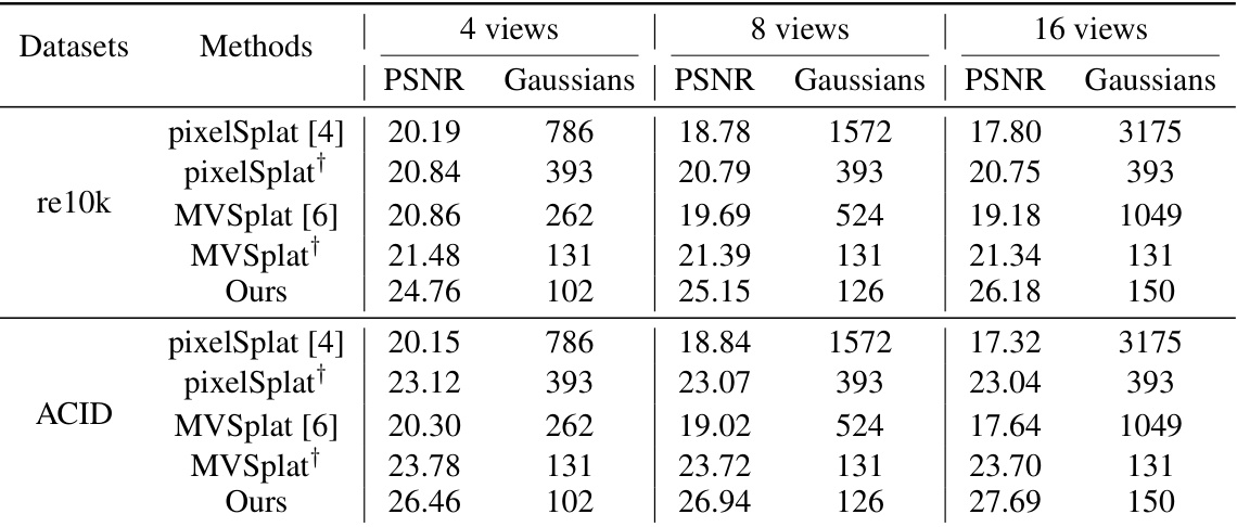
This table presents a quantitative comparison of different novel view synthesis methods (pixelSplat [4], MVSplat [6], and the proposed GGN) on two benchmark datasets, RealEstate10K and ACID. The comparison is based on Peak Signal-to-Noise Ratio (PSNR) and the number of Gaussians used for rendering novel views. Results are shown for 4, 8, and 16 input views. The † symbol indicates that methods using multiple views only use Gaussians from two views for the final rendering.
In-depth insights#
Gaussian Graph NN#
A Gaussian Graph Neural Network (GGNN) represents a novel approach to processing multi-view image data for efficient and generalizable 3D scene reconstruction. Instead of simply aggregating pixel-aligned Gaussians from different viewpoints, GGNN leverages a graph structure to model the relationships between groups of Gaussians. This allows for sophisticated message passing and feature fusion at the Gaussian level, enabling each Gaussian to benefit from contextual information provided by its neighbors in the graph. The key innovation lies in reformulating traditional graph operations to work directly on Gaussian representations, incorporating Gaussian-specific interactions. The network’s design also includes a Gaussian pooling layer for efficient representation aggregation, ultimately leading to higher quality renderings with fewer Gaussians compared to prior methods. This architecture demonstrates a potential advancement in 3D reconstruction by moving beyond simple aggregation and exploiting the underlying relationships inherent in multi-view data through graph-based reasoning. The scalability and generalization to unseen viewpoints are also key improvements claimed by the method.
Multi-view Fusion#
Multi-view fusion, in the context of 3D reconstruction from images, aims to combine information from multiple viewpoints to create a more complete and accurate 3D model. Effective strategies often leverage the geometric constraints inherent in multiple images, such as epipolar geometry. Successful fusion techniques must handle inconsistencies and noise present in individual images, while also being computationally efficient, especially when dealing with a high number of views. Different approaches exist, ranging from simple averaging to sophisticated deep learning methods. A key challenge is to resolve discrepancies between views, which can arise from differences in viewpoint, lighting, or object motion. Advanced techniques might involve cost volume construction, where matching costs are computed across views to infer depth maps. Another strategy uses graph neural networks to model inter-view dependencies and aggregate features intelligently. The optimal method often depends on factors such as the scene complexity, image quality, and computational resources available. Ultimately, the goal is to produce a unified representation that surpasses the accuracy and completeness of any single-view reconstruction.
Efficiency Analysis#
An efficiency analysis of a novel view synthesis method should meticulously examine its resource consumption, particularly focusing on computational cost and memory usage. The number of Gaussians used is a crucial metric, as it directly relates to model complexity and rendering speed. A reduction in the Gaussian count without compromising image quality is a significant achievement, demonstrating the algorithm’s effectiveness. The analysis should also consider the inference time, reporting results for various input settings and comparing them against state-of-the-art methods. Frames per second (FPS) is an important performance indicator for real-time applications. Furthermore, a comprehensive efficiency analysis must consider the trade-offs between computational cost and visual quality. The paper should investigate whether the method achieves comparable or better image quality with significantly lower computational demands, clearly showcasing its efficiency advantages.
Cross-Dataset Tests#
Cross-dataset tests are crucial for evaluating the generalizability of a model. They reveal how well a model, trained on one dataset, performs on unseen data from a different dataset. Strong performance on multiple datasets indicates robustness and less susceptibility to overfitting or biases specific to the training data. Conversely, poor performance highlights limitations and potential dataset-specific factors affecting the model. Analyzing these results provides insights into the model’s underlying assumptions and its ability to learn transferable features. Careful consideration should be given to the nature of the datasets used, ensuring diversity and addressing potential confounding factors that might explain any observed differences. For example, differences in image quality, annotation style, or data distribution between datasets could affect the model’s performance. Quantifying the impact of these factors is paramount to drawing meaningful conclusions. Therefore, thorough cross-dataset evaluation is an essential component for assessing the true capabilities and limitations of a machine learning model.
Future Directions#
The paper’s success in generating efficient and generalizable Gaussian representations opens exciting avenues. Future work could focus on handling higher-resolution inputs, addressing the current limitation of computational cost with increasing image size. This might involve exploring more efficient Gaussian representations or hierarchical structures. Improving robustness to noise and occlusions is also crucial for real-world applicability. The current model’s reliance on pixel-aligned Gaussians could be refined by incorporating more sophisticated scene understanding or incorporating other geometric primitives. Furthermore, extending the model to handle dynamic scenes would greatly increase its versatility and open up many applications. This could involve adapting the Gaussian Graph Network to handle temporal information or integrating it with existing neural representations of dynamic scenes. Finally, exploring the use of different graph neural network architectures might yield more efficient and powerful Gaussian representation learning.
More visual insights#
More on figures
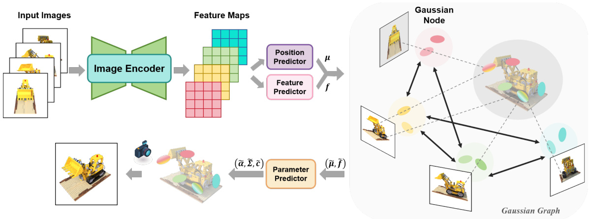
This figure illustrates the overall framework of the Gaussian Graph Network (GGN). It begins with multiple input images that are processed by an image encoder to generate feature maps. From these feature maps, a position predictor and feature predictor estimate the means (μ) and features (f) of pixel-aligned Gaussians. These Gaussians are then organized into a Gaussian Graph, where nodes represent groups of Gaussians and edges represent relationships between them. A Gaussian Graph Network processes this graph to fuse information between Gaussians before a parameter predictor generates the final Gaussian parameters (α, Σ, č).

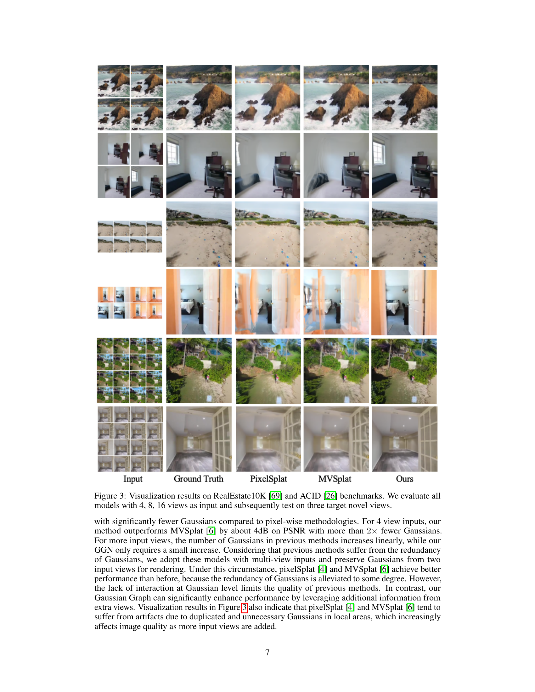
This figure shows a comparison of novel view synthesis results from different methods (PixelSplat, MVSplat, and the proposed GGN method) using 4, 8, and 16 input views. The ground truth images are also provided for reference. Each row represents a different scene, showcasing the rendered images produced by each method. The results highlight the visual quality and differences in the number of Gaussians used by each approach, with the GGN method demonstrating improved quality with fewer Gaussians.
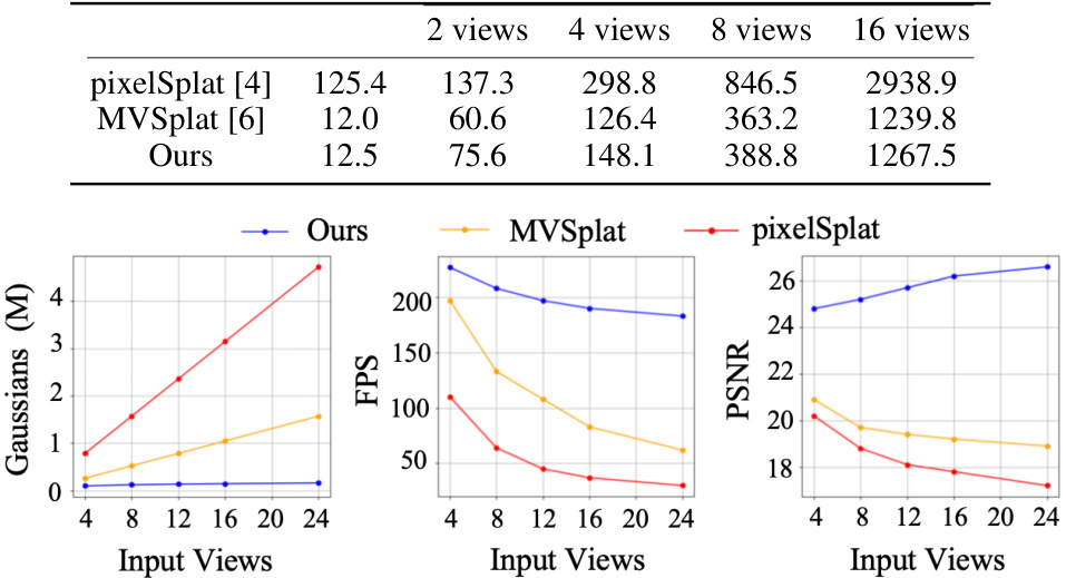
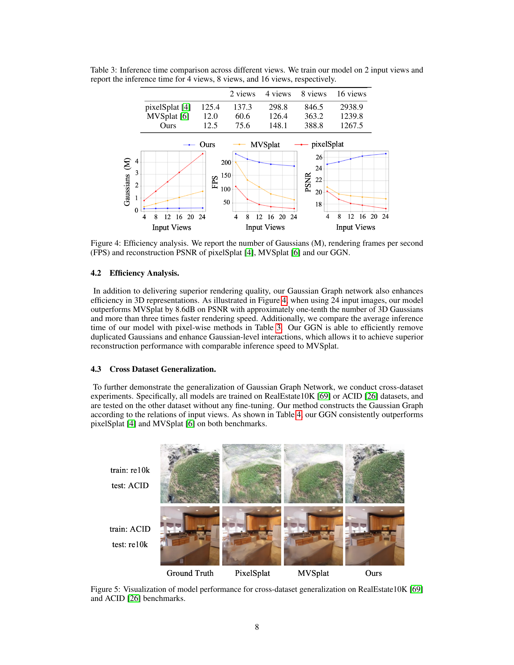
This figure analyzes the efficiency of the proposed Gaussian Graph Network (GGN) compared to two existing methods, pixelSplat and MVSplat. It shows the trade-off between the number of Gaussians used (a measure of model complexity and memory usage), the rendering speed (frames per second, FPS), and the resulting image quality (Peak Signal-to-Noise Ratio, PSNR). The results demonstrate that GGN achieves higher PSNR (better image quality) with fewer Gaussians and faster rendering speed than the other methods.
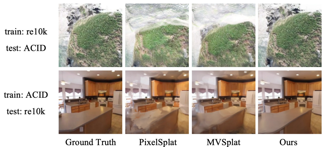
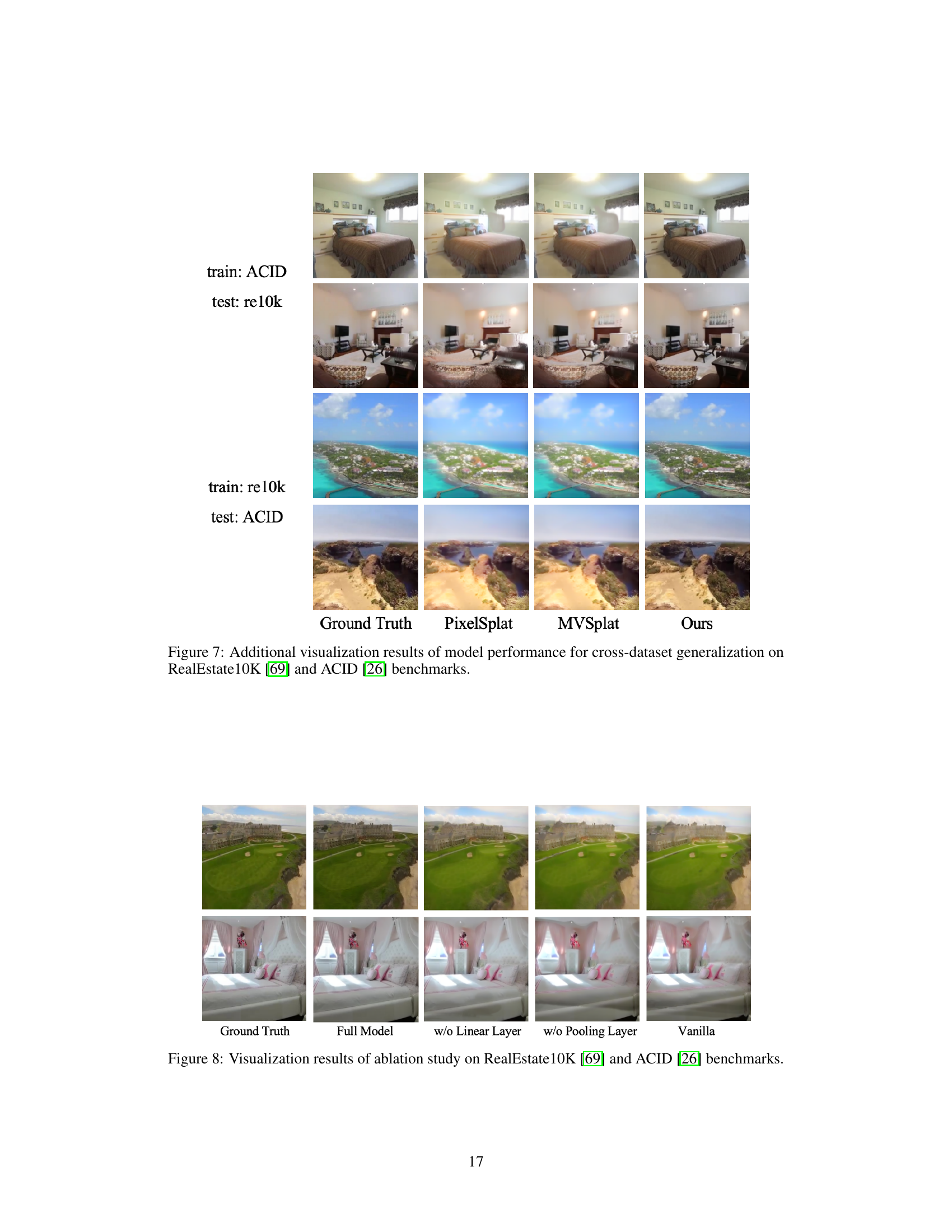
This figure shows the results of a cross-dataset generalization experiment. The model was trained on either the RealEstate10K or ACID dataset and then tested on the other dataset. The top row displays results when trained on RealEstate10K and tested on ACID, and the bottom row displays the inverse. Each column shows the ground truth, PixelSplat, MVSplat and the proposed GGN method. The figure aims to demonstrate the generalization capability of the GGN across different datasets.
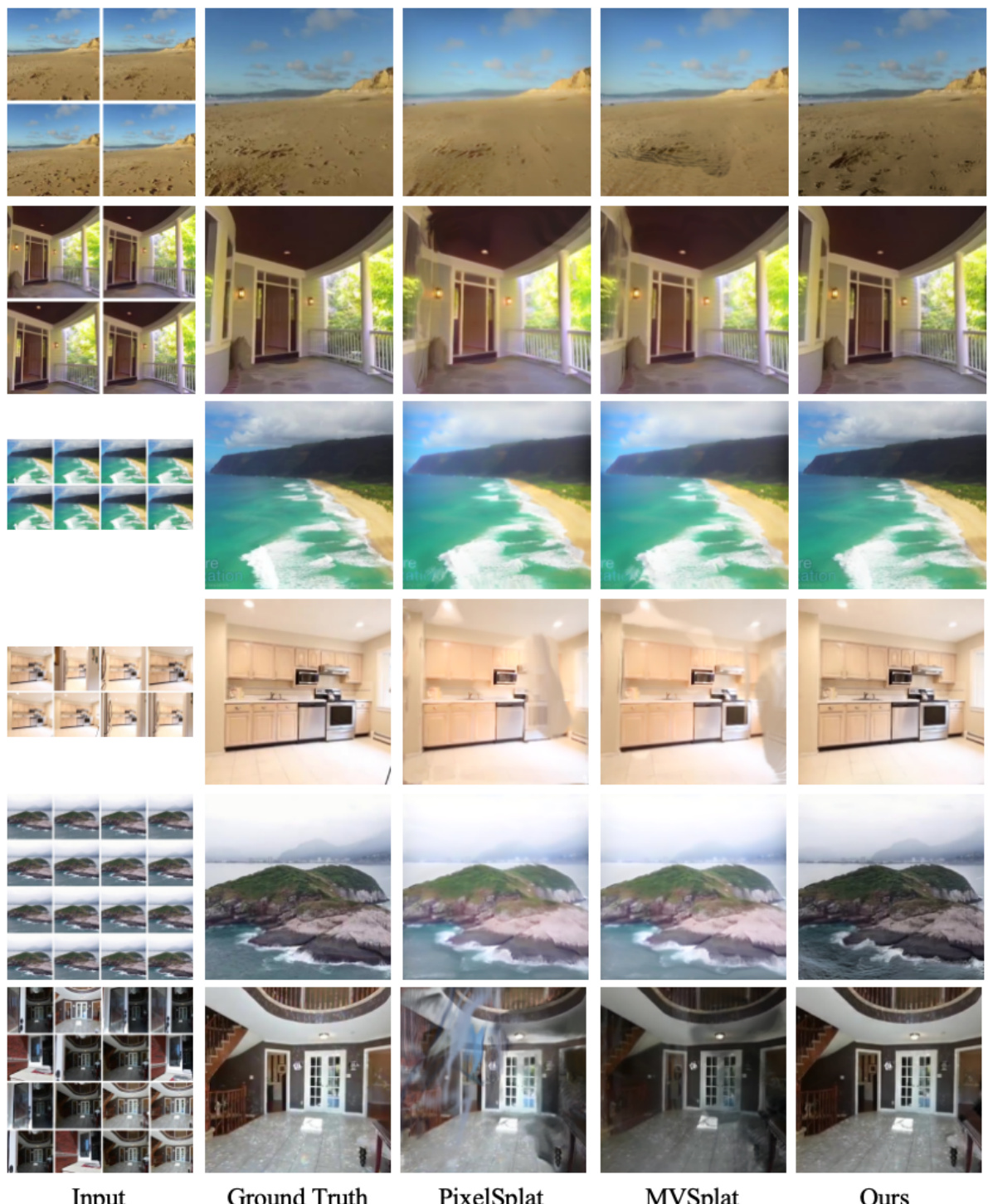
This figure displays a comparison of novel view synthesis results from various methods, including PixelSplat, MVSplat, and the proposed Gaussian Graph Network (GGN). Each row represents a different scene, showing input views (leftmost), ground truth (second from left), results from PixelSplat, MVSplat, and finally, the results from GGN. The figure visually demonstrates the superior image quality and efficiency achieved by GGN compared to the baseline methods, particularly as the number of input views increases. The differences highlight GGN’s ability to generate more realistic novel views with fewer artifacts, even with limited input data.
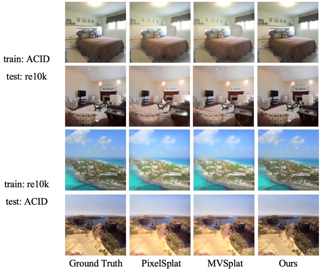
This figure shows the cross-dataset generalization results of the proposed Gaussian Graph Network (GGN) method. The model is trained on either the RealEstate10K or ACID dataset and then tested on the other dataset, demonstrating its ability to generalize across different scene types. The results are compared against the ground truth and two other state-of-the-art methods, pixelSplat and MVSplat, showcasing the superior performance of GGN.
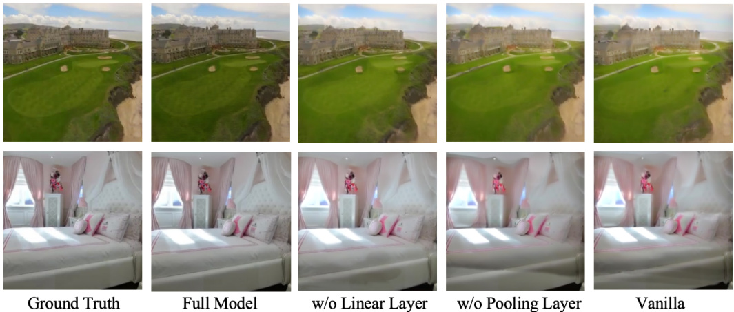
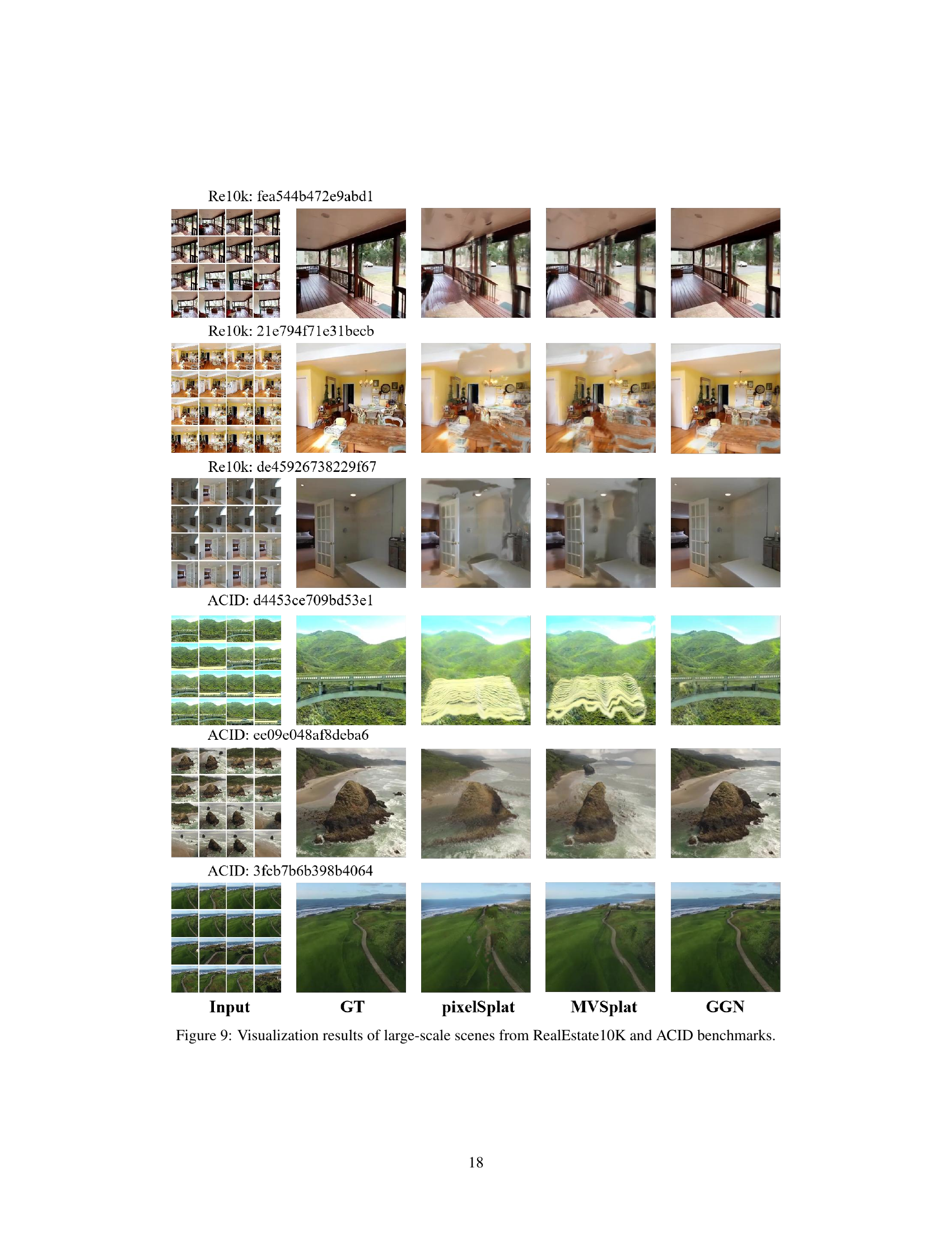
This figure presents an ablation study comparing the performance of the proposed Gaussian Graph Network (GGN) with several variants. The ‘Full Model’ represents the complete GGN. ‘w/o Linear Layer’ shows the results when the linear layers are removed from the GGN. ‘w/o Pooling Layer’ omits the pooling layers. Finally, ‘Vanilla’ denotes a baseline model without the Gaussian Graph architecture. The visualizations demonstrate the impact of each component of the GGN on the final image quality.
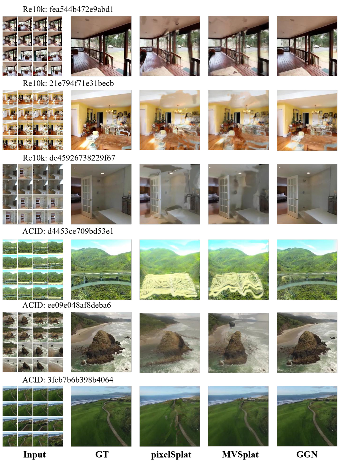
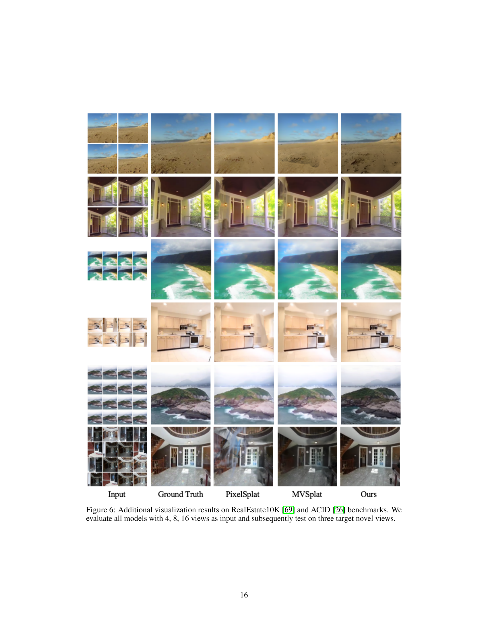
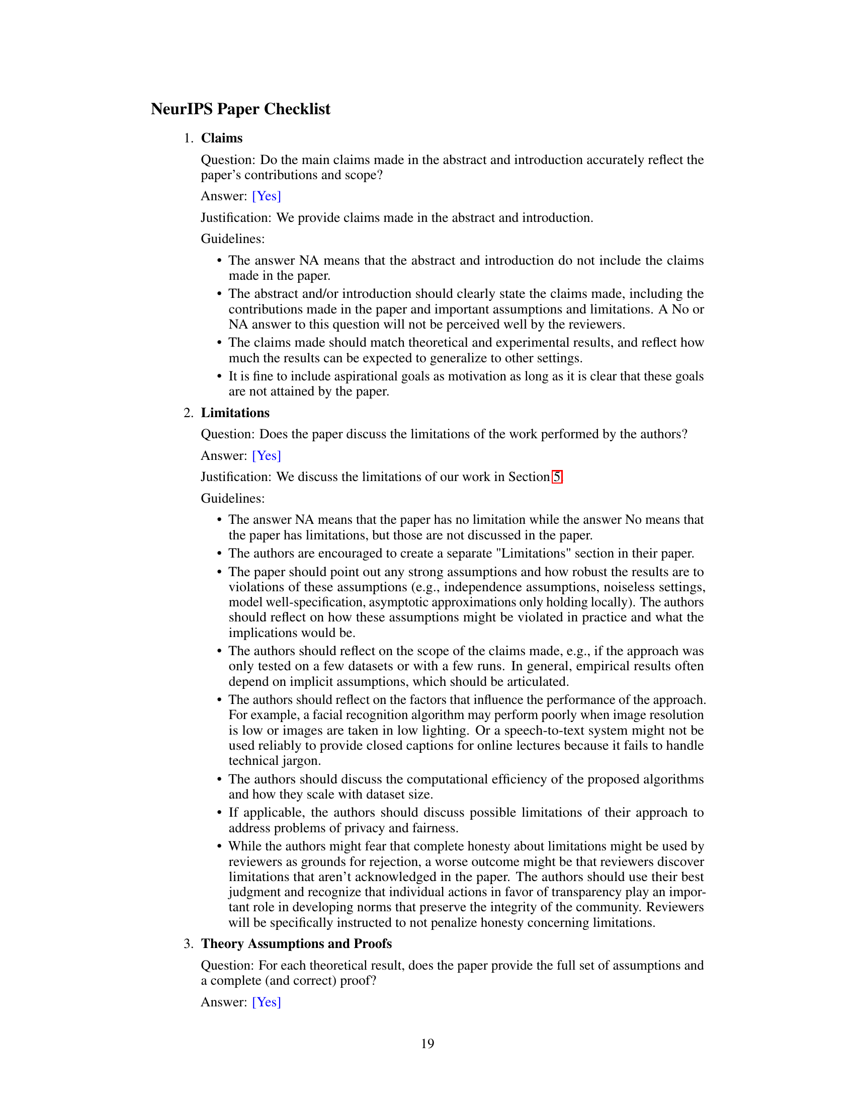
This figure shows a comparison of novel view synthesis results on six large-scale scenes from the RealEstate10K and ACID datasets. For each scene, it displays the input images, the ground truth, and the results from three different methods: PixelSplat, MVSplat, and the authors’ proposed GGN (Gaussian Graph Network) method. The visualization demonstrates the ability of each method to generate novel views from multiple input images, and highlights the differences in visual quality between the approaches, particularly with regard to detail preservation and artifact reduction.
More on tables

This table presents a comparison of the performance of different novel view synthesis methods using only two input views. The average PSNR, SSIM, and LPIPS scores are reported for each method across all test scenes in the RealEstate10K and ACID datasets. The metrics evaluate the quality of the synthesized novel views generated from the input views.

This table presents a quantitative comparison of the proposed Gaussian Graph Network (GGN) and two baseline methods (pixelSplat and MVSplat) on cross-dataset generalization tasks. It shows the performance of models trained on one dataset (either RealEstate10K or ACID) and tested on the other dataset. The metrics reported include PSNR, SSIM, LPIPS, the number of Gaussians used, and Frames Per Second (FPS). This demonstrates the generalizability and efficiency of the GGN.

This ablation study analyzes the impact of key components within the Gaussian Graph Network (GGN) architecture on the model’s performance. By systematically removing components such as the Gaussian Graph linear layer and Gaussian Graph pooling layer, the study isolates the contribution of each component towards the overall performance. The ‘Vanilla’ model represents the baseline without any of the proposed GGN components. The results quantitatively demonstrate the importance of each component in achieving better performance. The metrics used are PSNR, SSIM, LPIPS and the number of Gaussians used.

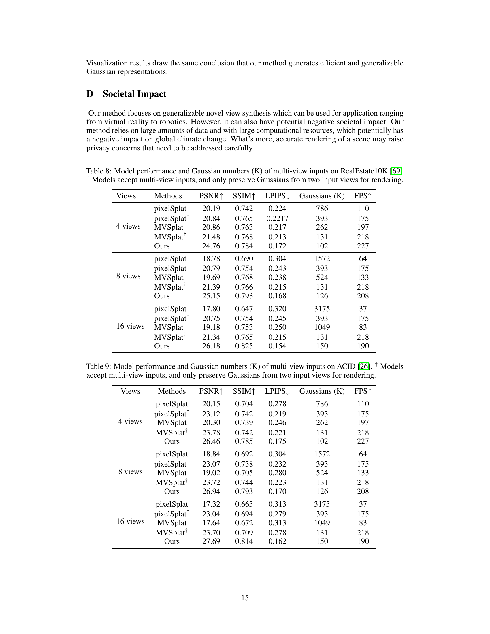
This table presents a quantitative comparison of different novel view synthesis methods on two benchmark datasets: RealEstate10K and ACID. The methods are evaluated using 4, 8, and 16 input views, and the results are reported in terms of Peak Signal-to-Noise Ratio (PSNR) and the number of Gaussians used for rendering. The table highlights the efficiency gains of the proposed Gaussian Graph Network (GGN) method, which achieves comparable or better PSNR with significantly fewer Gaussians.

This table presents a quantitative comparison of different novel view synthesis methods on the RealEstate10K and ACID benchmark datasets. The methods are evaluated using 4, 8, and 16 input views. The table reports the Peak Signal-to-Noise Ratio (PSNR) and the number of Gaussians used for rendering. Note that methods marked with † use multiple views as input but only render using Gaussians from two of the input views.
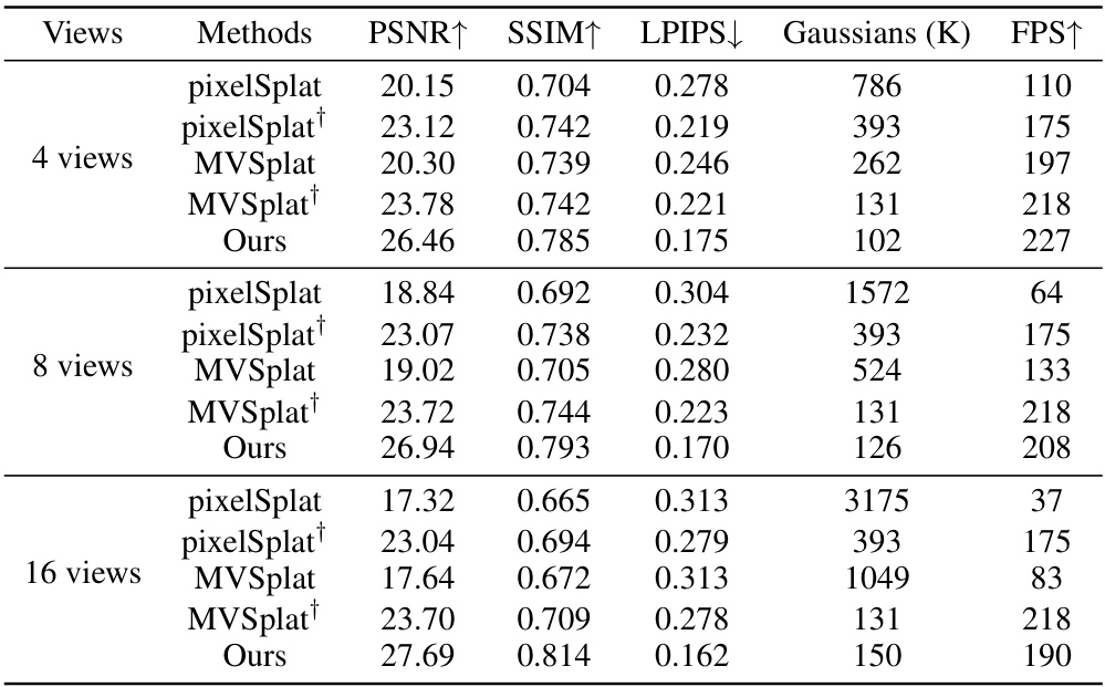
This table presents a quantitative comparison of different novel view synthesis methods (pixelSplat, MVSplat, and the proposed GGN) on the RealEstate10K and ACID datasets. The comparison is based on Peak Signal-to-Noise Ratio (PSNR) and the number of Gaussians used in the models’ representations for 4, 8, and 16 input views. Note that for methods that handle multiple views, the results are shown for using only two views for final rendering to ensure a fair comparison.
Full paper#
