↗ OpenReview ↗ NeurIPS Homepage ↗ Chat
TL;DR#
Many inverse problems, prevalent in various fields like image processing and audio engineering, aim to recover original data from incomplete or noisy observations. Existing methods integrating diffusion models often neglect their powerful denoising capabilities, limiting their effectiveness. This paper tackles this limitation head-on.
The proposed ProjDiff algorithm ingeniously recasts noisy inverse problems as a constrained optimization task, introducing an auxiliary variable to represent a noisy sample. This allows the algorithm to efficiently utilize both the prior information and denoising power of pre-trained diffusion models. ProjDiff demonstrates superior performance across diverse linear and non-linear inverse problems, establishing a new benchmark and showing the potential of fully exploiting diffusion models’ denoising ability for accurate and efficient inverse problem solutions.
Key Takeaways#
Why does it matter?#
This paper is crucial for researchers working on inverse problems because it introduces a novel method, ProjDiff, that significantly improves the performance of solving these problems. ProjDiff effectively leverages the denoising capability of pre-trained diffusion models, which has been largely overlooked by previous approaches. This opens exciting new avenues for applying diffusion models to various linear and non-linear inverse problems, impacting diverse fields such as image restoration, source separation, and audio processing.
Visual Insights#

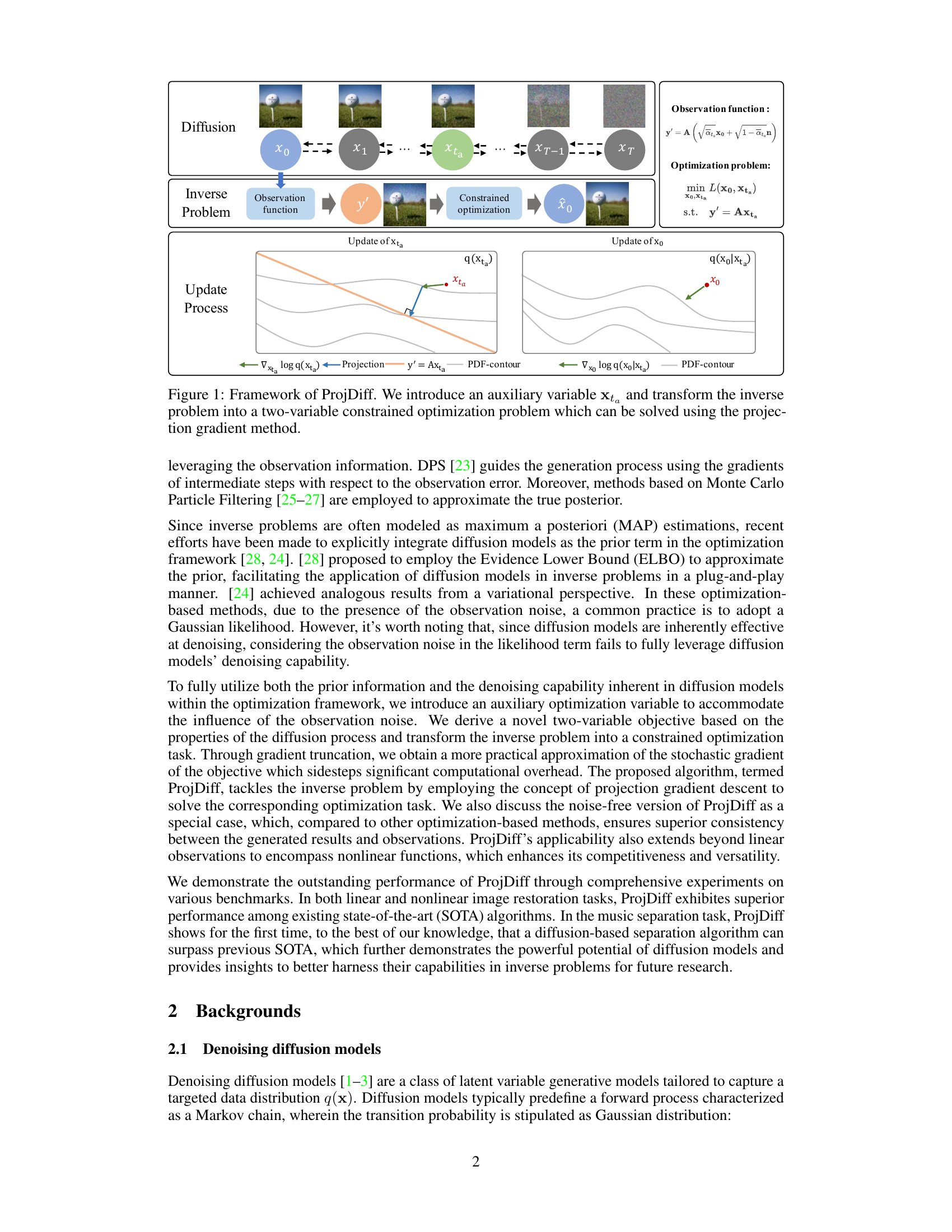
The figure illustrates the framework of the proposed ProjDiff algorithm for solving inverse problems. It shows how a diffusion model’s denoising capability is integrated with an optimization process. The inverse problem is transformed into a constrained optimization problem using an auxiliary variable xta representing a noisy sample at a specific step in the diffusion process. The solution involves iterative updates of both the original variable x0 and the auxiliary variable xta. The update process for xta is constrained by the observation equation, and uses projection gradient descent, shown visually as a projection onto the constraint. The update for x0 leverages the denoising capability of the diffusion process to refine the estimate towards the noise-free solution. The PDF contours visualize the probability density functions involved in the optimization.

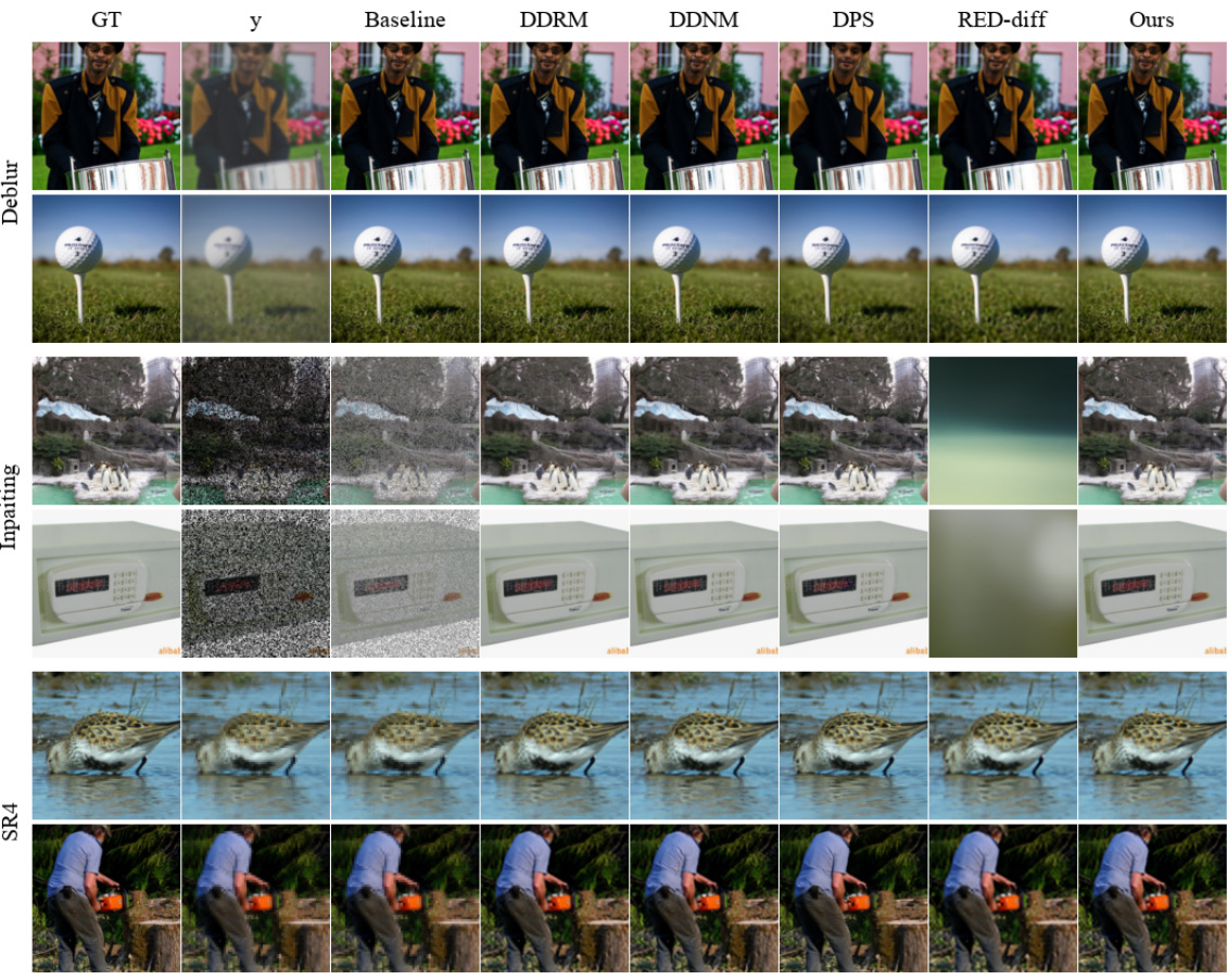
This table presents the performance comparison of different methods on three linear image restoration tasks (super-resolution, inpainting, and Gaussian deblurring) on the ImageNet dataset with Gaussian noise (σ = 0.05). The metrics used for evaluation are PSNR, SSIM, LPIPS (multiplied by 100 for easier readability), and FID. The results show the performance of ProjDiff compared to other state-of-the-art methods (DPS, DDRM, DDNM+, RED-diff).
In-depth insights#
Diffusion Priors#
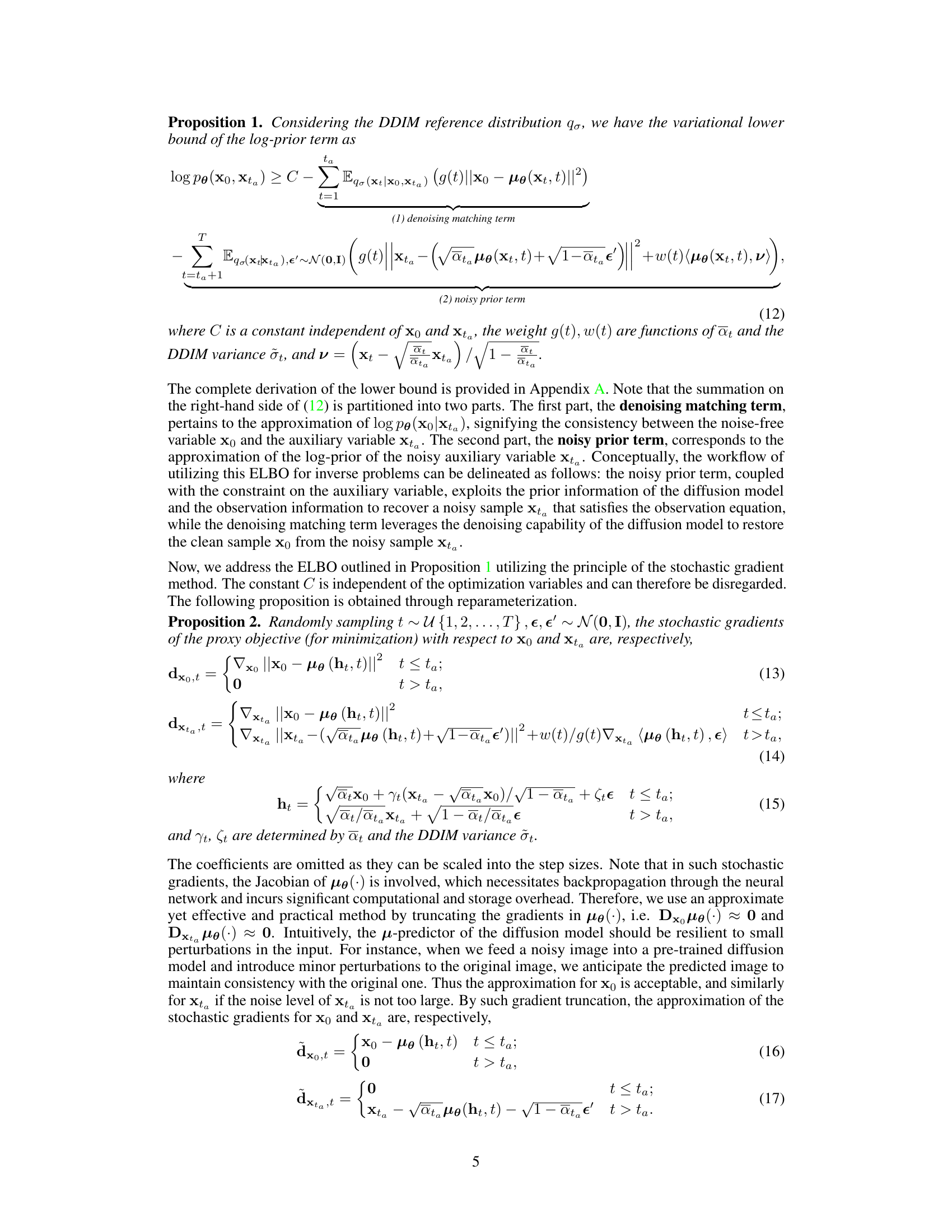
Diffusion models have emerged as powerful generative models, capable of learning complex data distributions. Their application as learnable priors in solving inverse problems is a significant advancement. Instead of solely using the prior information within the diffusion models, a key insight is to leverage their denoising capabilities. This involves reframing inverse problems as optimization tasks that incorporate an auxiliary variable representing a ’noisy’ sample within the diffusion process. This approach facilitates the efficient integration of both prior information and denoising, leading to superior performance in solving various inverse problems. The algorithm proposed effectively balances these aspects, enabling improved image restoration, source separation, and partial data generation. The approach is also generalized to handle nonlinear inverse problems. Future work could explore more sophisticated methods of incorporating the denoising properties of diffusion models to further enhance performance and address the limitations of current optimization techniques.
ProjDiff Algorithm#
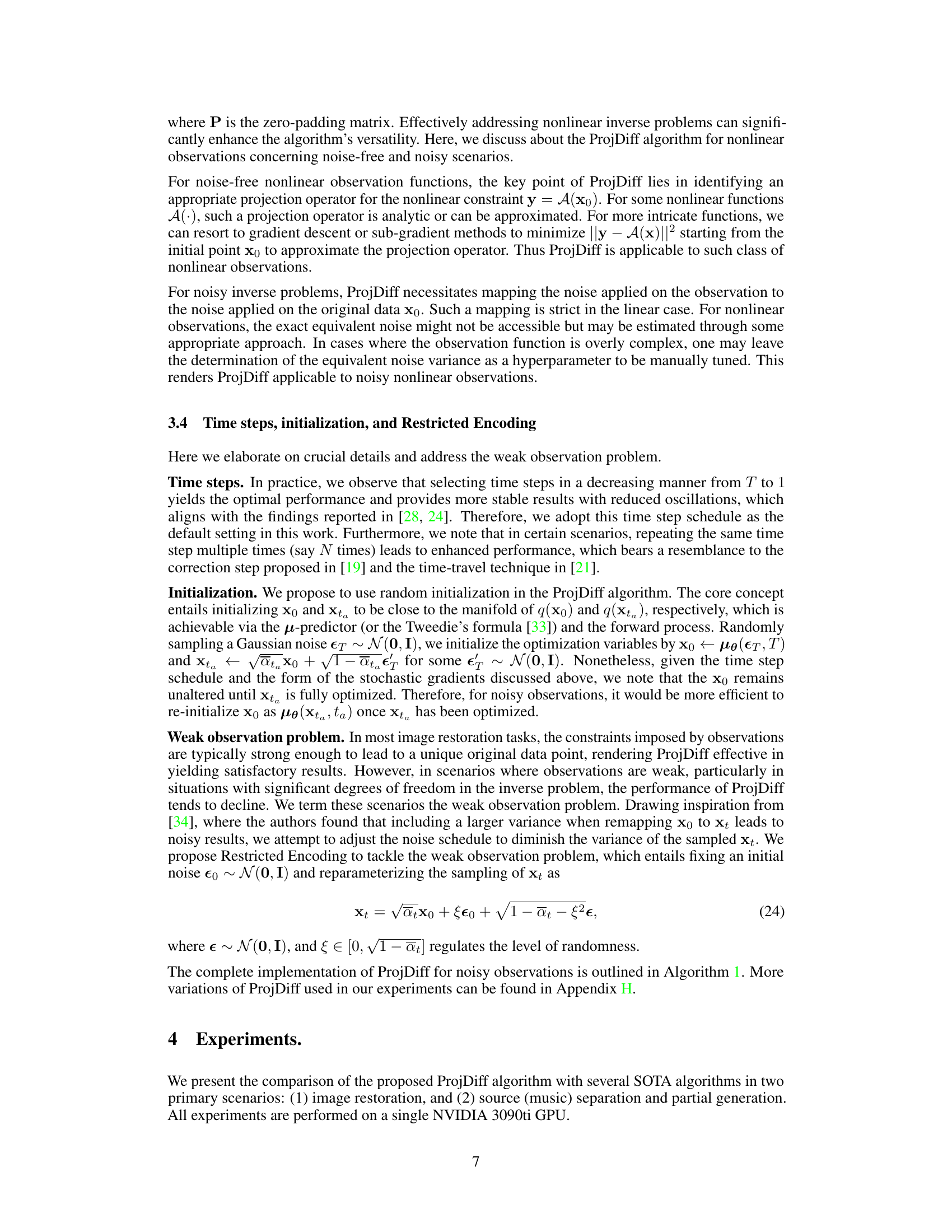
The ProjDiff algorithm ingeniously tackles inverse problems by leveraging the denoising capabilities of pre-trained diffusion models. Instead of solely relying on optimization methods that utilize prior information, ProjDiff introduces an auxiliary variable representing a ’noisy’ sample at an equivalent denoising step. This reformulates the problem as a two-variable constrained optimization task, efficiently solved by the projection gradient descent method. Truncating the gradient through the µ-predictor enhances efficiency. The algorithm’s strength lies in its ability to seamlessly integrate prior knowledge and denoising, thereby demonstrating superior performance across linear and nonlinear inverse problems, including image restoration and source separation. The innovative use of an auxiliary variable effectively handles observation noise and unlocks the full potential of diffusion models for solving a broad range of challenging inverse problems.
Nonlinear Tasks#
The section on “Nonlinear Tasks” would likely delve into the challenges and solutions of applying diffusion models to inverse problems where the relationship between the observed data and the underlying signal is nonlinear. This is a significant departure from the simpler linear scenarios, where a direct linear transformation exists. Nonlinearity introduces complexities in modeling the data distribution and designing efficient optimization strategies. The authors likely present a novel method or adaptation of their core algorithm to handle nonlinear observations, which may involve techniques like carefully crafted transformations to approximate linearity or incorporating nonlinear functions directly within their optimization framework. Performance comparisons against existing state-of-the-art methods, specifically designed for nonlinear inverse problems, would be crucial to demonstrate the effectiveness and novelty of the proposed approach. The experimental results would show improved performance in challenging scenarios, such as phase retrieval or high dynamic range (HDR) image restoration. Detailed qualitative and quantitative analyses would likely showcase improvements in both reconstruction quality and efficiency compared to baseline methods. The success in addressing nonlinear scenarios would highlight the algorithm’s robustness and versatility in practical applications.
Future Research#
The paper’s conclusion points toward several promising avenues for future research. Extending ProjDiff’s applicability to non-Gaussian noise models (e.g., Poisson, multiplicative noise) is crucial for broader real-world application. The current reliance on Gaussian noise limits its versatility. Further investigation into adaptive step size strategies would enhance ProjDiff’s efficiency and reduce the need for manual parameter tuning. The authors also suggest exploring more computationally efficient approximations for the stochastic gradients, potentially through techniques that bypass the Jacobian calculations of the μ-predictor. Finally, research should focus on developing methods to more effectively handle weak observation scenarios where the information provided by the observation is insufficient to uniquely determine the original data. Addressing these limitations would significantly improve ProjDiff’s robustness and expand its applicability to a wider range of inverse problems.
Algorithm Limits#
An ‘Algorithm Limits’ section in a research paper would critically examine the boundaries of the proposed method’s applicability and performance. This would involve discussing computational complexity, scalability limitations, and potential failure modes. For example, it should address whether the algorithm performs well with high-dimensional data or extremely noisy observations, and whether its runtime scales favorably with increasing data size or model complexity. The robustness to outliers or adversarial examples would also be crucial. A complete analysis must identify the types of problems where the algorithm excels and where it struggles, providing a realistic assessment of its strengths and weaknesses and emphasizing its limitations in specific contexts to fully inform potential users. It’s also vital to note any assumptions made about the data or model parameters that limit generalizability and potential biases introduced by the algorithm itself. Finally, the section should suggest avenues for future work to address these limitations, potentially proposing modifications or alternative approaches to extend the algorithm’s reach and applicability.
More visual insights#
More on figures

This figure shows the results of noise-free nonlinear restoration on the FFHQ dataset with σ = 0. It compares the performance of different methods, including DPS, RED-diff, and ProjDiff, on restoring images from their noisy or incomplete observations. The ‘GT’ column displays the ground truth images, ‘y’ shows the noisy or incomplete observations, and subsequent columns display the reconstruction results from each method. This provides a visual comparison of the restoration quality achieved by each method on various types of nonlinear inverse problems.

This figure visualizes the performance of ProjDiff (and other compared algorithms) on the ImageNet super-resolution task. The x-axis represents either FID or LPIPS, and the y-axis represents PSNR. Each point represents an algorithm’s performance. The red lines trace the change in PSNR across different FID and LPIPS values for the ProjDiff algorithm, showing how PSNR changes with different hyperparameter settings (step size). This illustrates the trade-off between the perceptual metrics (LPIPS, FID) and objective metric (PSNR) that can be achieved by tuning the hyperparameters.

This figure shows a comparison of audio waveforms generated by three different source separation methods: ProjDiff, RED-diff, and MSDM. Each row represents a different audio track from a mixed audio source. The figure visually demonstrates that ProjDiff tends to produce audio with higher amplitude than the other two methods; RED-diff and MSDM often have more periods of silence. This supports the claim that ProjDiff outperforms other methods in terms of scale-invariant SDR improvement (SI-SDRi).
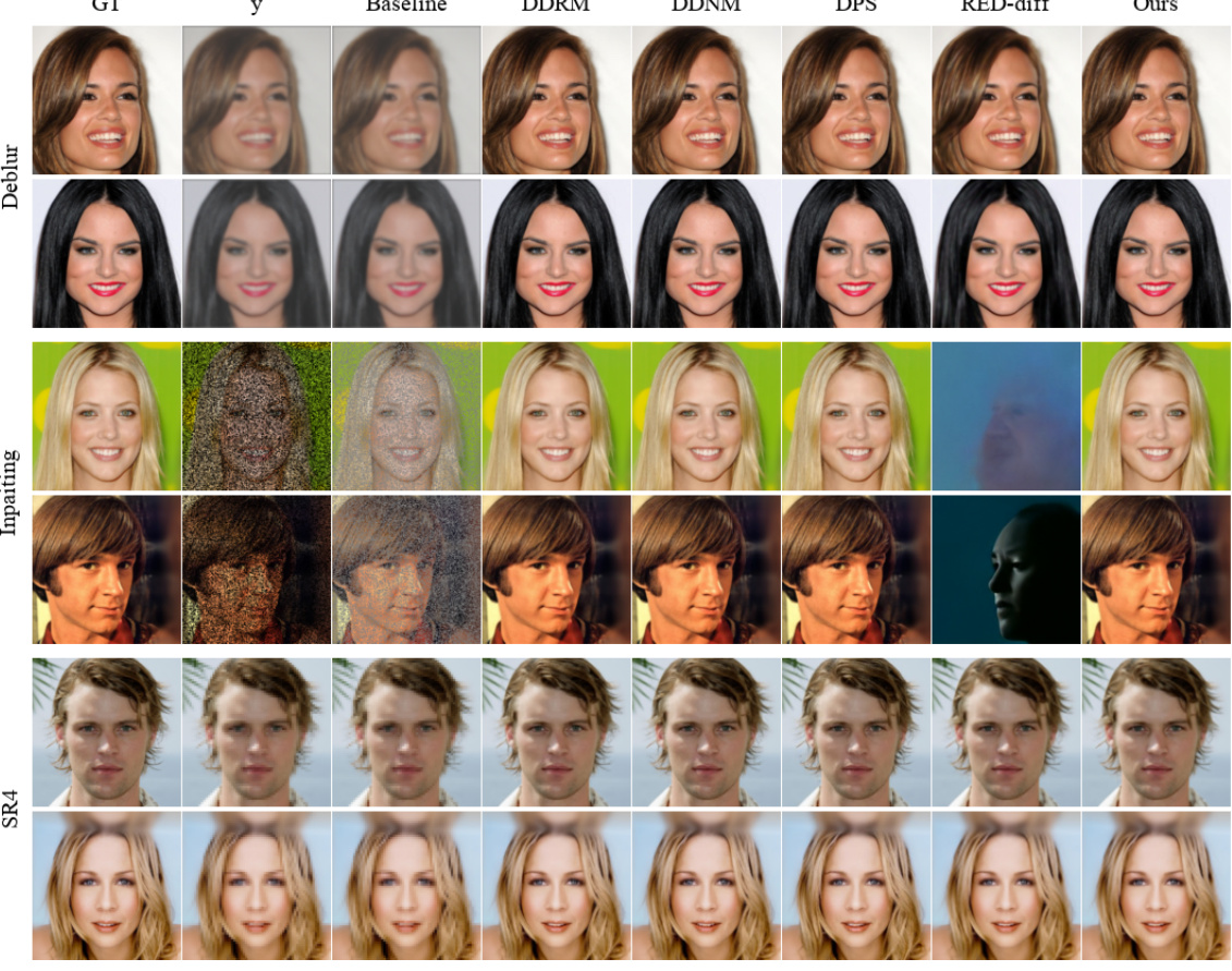
This figure shows the results of linear image restoration on the CelebA dataset with a noise standard deviation of 0.05. It compares the performance of several methods: a baseline method (least squares solution), DDRM, DDNM, DPS, RED-diff, and the proposed ProjDiff method. Each row represents a different type of restoration task: super-resolution, inpainting, and deblurring. The ground truth image (GT) and the noisy observation (y) are shown alongside the results of each method. The comparison highlights the performance improvement achieved by ProjDiff.

This figure shows a comparison of linear image restoration results on the CelebA dataset using different methods. The standard deviation of the added Gaussian noise is 0.05. The results are shown for three tasks: super-resolution (SR4), inpainting, and deblurring. The ‘GT’ column displays the ground truth images. The ‘y’ column shows the noisy observations. The ‘Baseline’ column represents the results obtained using the least squares solution (x0 = A†y). The remaining columns show the results obtained using DDRM, DDNM, DPS, RED-diff, and the proposed ProjDiff method, respectively. The figure visually demonstrates the superior performance of ProjDiff in restoring the images compared to other state-of-the-art algorithms.
This figure displays the results of linear image restoration experiments conducted on the CelebA dataset with a noise level (σ) of 0.05. The image restoration tasks involved are deblurring, inpainting, and super-resolution (SR4). Each row showcases the results for a single image, starting with the ground truth (GT) image, followed by the degraded observation (y), the result of a least-squares solution (Baseline), and then the results obtained using the DDRM, DDNM, DPS, RED-diff, and ProjDiff algorithms. This allows for a visual comparison of the performance of the different methods across various linear inverse problems.
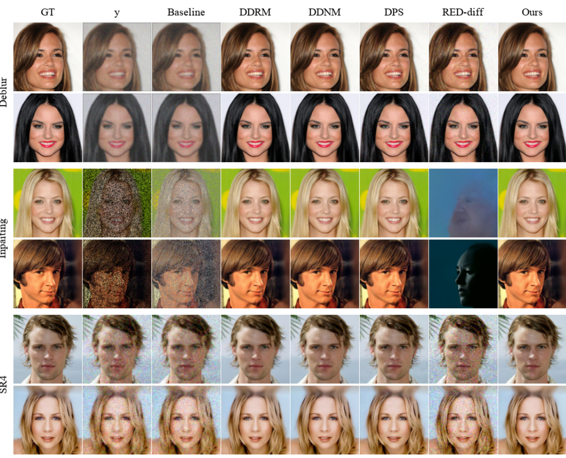
This figure shows the results of linear image restoration on the CelebA dataset using different methods. The noise level (sigma) is 0.05. The top row displays the ground truth images, the second row shows the observed (noisy) images, and the remaining rows present the results obtained by different restoration algorithms. The ‘Baseline’ represents a simple least-squares solution.

This figure showcases the results of noise-free nonlinear image restoration on the FFHQ dataset using different methods. It compares the ground truth (GT) images with the observed images (y) and the restored images obtained using DPS, RED-diff, and the proposed ProjDiff algorithm. The comparison is performed on three different nonlinear inverse problems: HDR, and Phase Retrieval. Each row represents a different image, and the columns show the different stages: GT, the observation (y), and the restoration results for the compared algorithms.
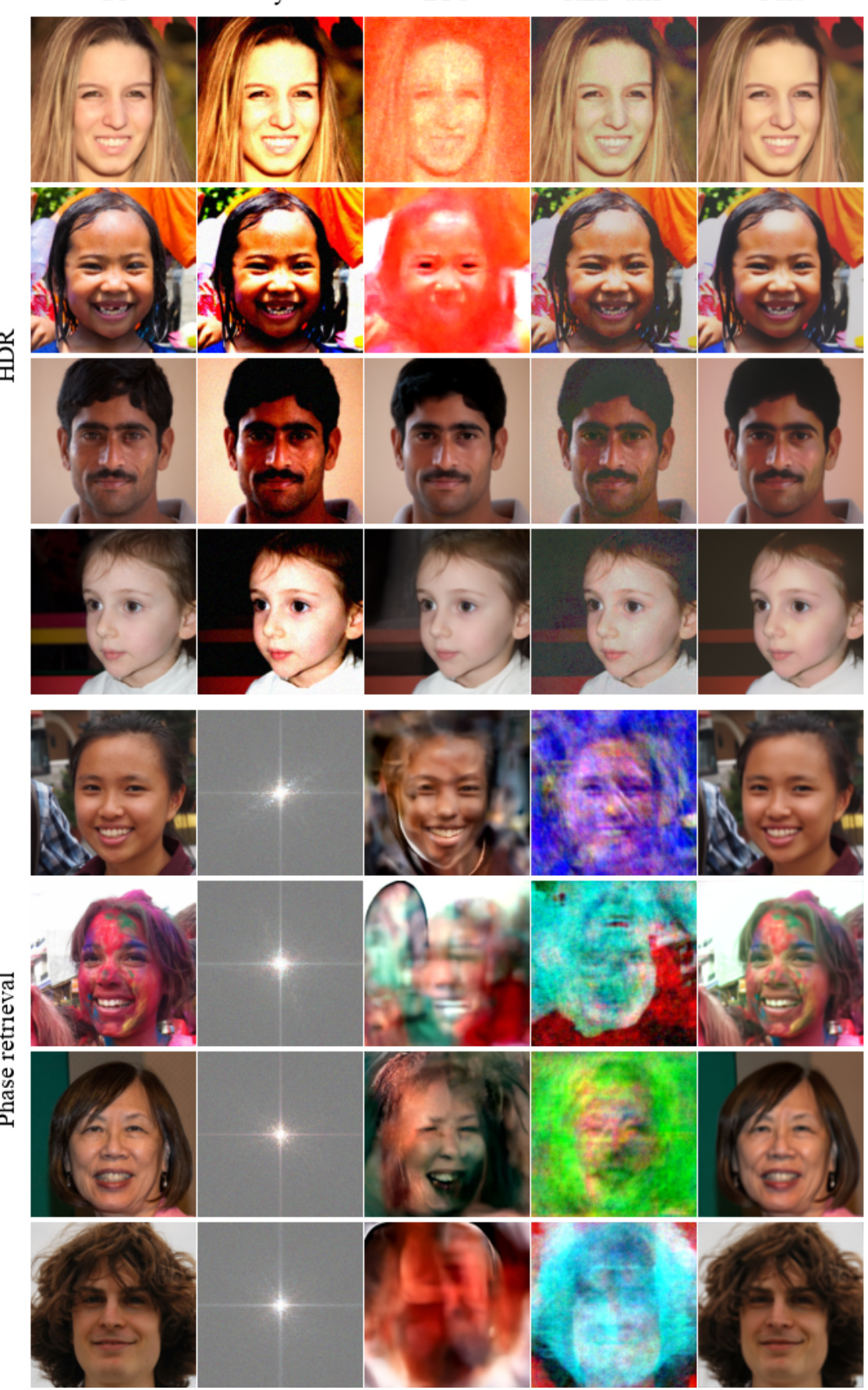
This figure shows the results of noise-free nonlinear image restoration on the FFHQ dataset, comparing the performance of different methods. The ‘GT’ column shows the ground truth images. The ‘y’ column displays the noisy or degraded input images. The remaining columns present the results of DPS, RED-diff, and ProjDiff, respectively. The figure allows a visual comparison of the restoration quality obtained by each method on a variety of faces.
More on tables
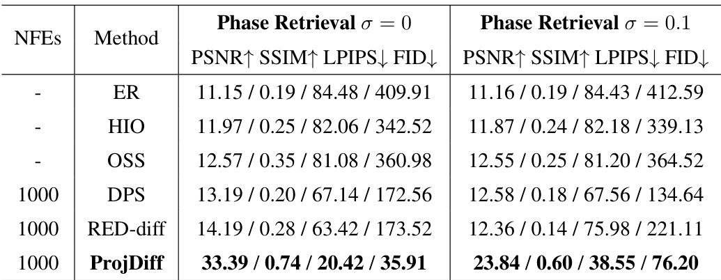
This table presents the performance comparison of different phase retrieval algorithms (ER, HIO, OSS, DPS, RED-diff, and ProjDiff) under two scenarios: noise-free (σ = 0) and noisy (σ = 0.1). The performance metrics reported include PSNR, SSIM, LPIPS (multiplied by 100), and FID. The NFES column indicates the number of function evaluations used by each algorithm. The results demonstrate ProjDiff’s superior performance, especially in the noise-free scenario.

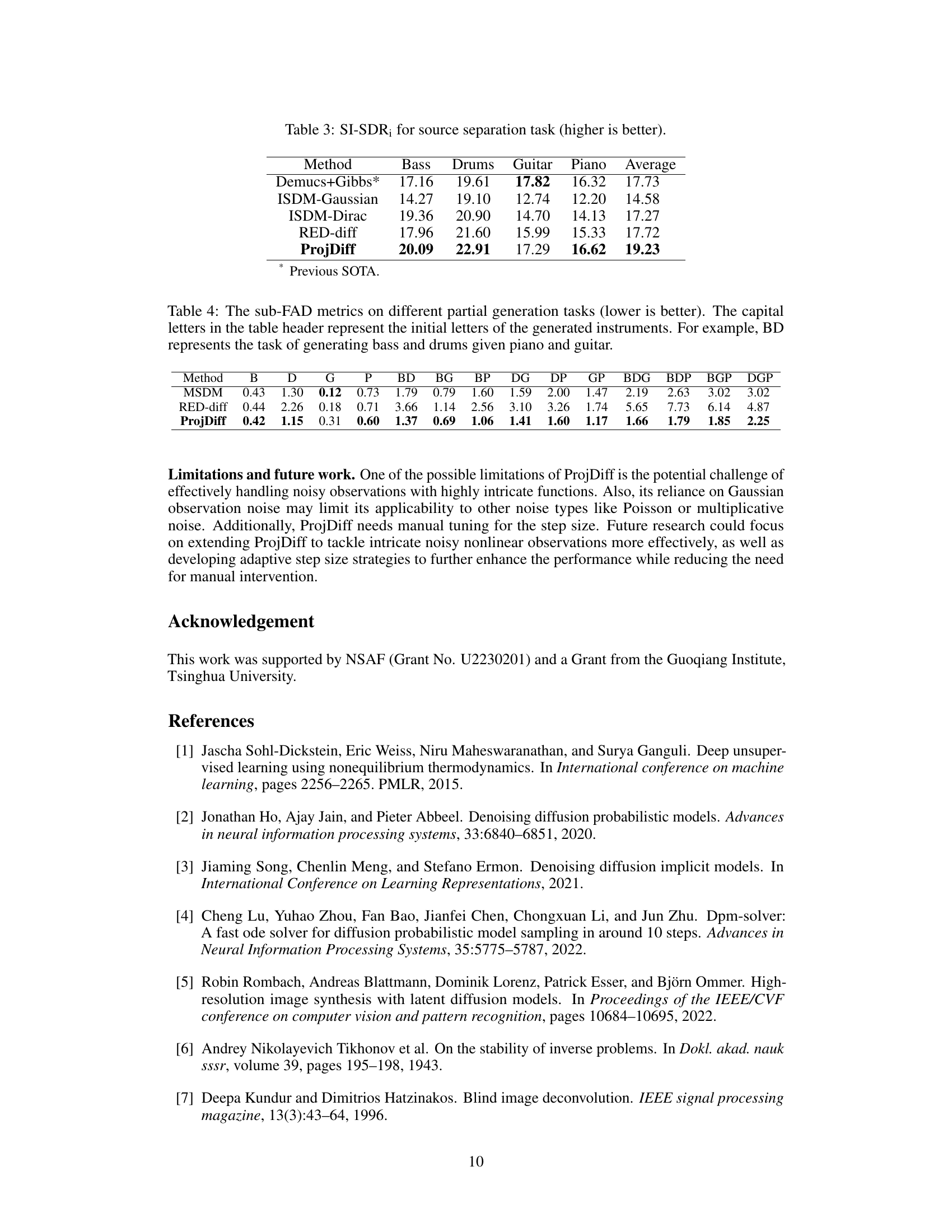
This table presents the scale-invariant SDR improvement (SI-SDRi) scores for a source separation task. The task involves separating four instruments (bass, drums, guitar, piano) from a mixed audio sequence. The table compares the performance of ProjDiff against several other methods, including Demucs+Gibbs (a previous state-of-the-art), ISDM-Gaussian, ISDM-Dirac, and RED-diff. Higher SI-SDRi values indicate better separation performance. The ‘Average’ column provides an overall performance score across all four instruments.

This table presents the results of the partial generation task, which aims to generate tracks of other instruments given partial tracks of some instruments. The results are evaluated using the sub-FAD metric, a lower score indicating better performance. Each column represents a different partial generation task, denoted by a combination of capital letters representing the instruments; for example, BD means generating bass and drums given piano and guitar. The table compares the performance of different methods, including MSDM, RED-diff, and ProjDiff.

This table presents the performance comparison of different methods on noisy image restoration tasks using the ImageNet dataset with a noise standard deviation of 0.05. The metrics used for evaluation include Peak Signal-to-Noise Ratio (PSNR), Structural Similarity Index (SSIM), Learned Perceptual Image Patch Similarity (LPIPS), and Frechet Inception Distance (FID). LPIPS values are multiplied by 100 for easier readability. The methods compared include a baseline (A†y), DPS, DDRM, DDNM+, RED-diff, and the proposed ProjDiff method. The number of function evaluations (NFES) is also specified for each method.

The table presents the performance comparison of different image restoration algorithms on the ImageNet dataset with noise (standard deviation = 0.05). The algorithms are evaluated using four metrics: PSNR (Peak Signal-to-Noise Ratio), SSIM (Structural Similarity Index), LPIPS (Learned Perceptual Image Patch Similarity), and FID (Fréchet Inception Distance). The LPIPS scores are multiplied by 100 for easier readability. The results show the effectiveness of ProjDiff compared to other state-of-the-art methods across three image restoration tasks: super-resolution, inpainting, and Gaussian deblurring.
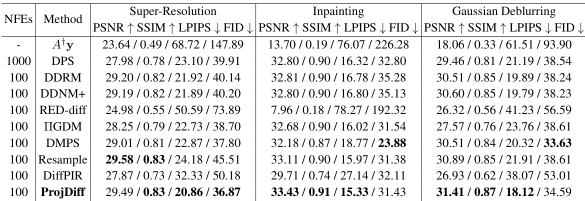
This table presents the performance comparison of different methods on the noisy image restoration task using the ImageNet dataset with a noise level (standard deviation) of 0.05. The metrics used for evaluation are PSNR, SSIM, LPIPS (multiplied by 100 for easier readability), and FID. The table compares the performance of ProjDiff against several state-of-the-art (SOTA) methods including A†y (least squares solution), DPS, DDRM, DDNM+, and RED-diff, across three different linear image restoration tasks: super-resolution, inpainting, and Gaussian deblurring.

This table presents the performance of different methods on the phase retrieval task with two different noise levels (σ = 0 and σ = 0.1). The metrics used for evaluation are PSNR, SSIM, LPIPS (multiplied by 100), and FID. The results show a comparison between ProjDiff and other baseline and state-of-the-art algorithms such as ER, HIO, OSS, DPS, and RED-diff. The number of function evaluations (NFES) is also specified.

This table presents a comparison of the performance of DDRM, DDNM, and ProjDiff on three linear image restoration tasks (super-resolution, inpainting, and Gaussian deblurring) using only 20 steps. The metrics used to evaluate the performance are PSNR, SSIM, LPIPS (multiplied by 100), and FID. The results demonstrate ProjDiff’s competitive performance, even with a significantly reduced number of steps.

This table presents the performance comparison of several image restoration algorithms on the ImageNet dataset with Gaussian noise (σ = 0.05). The algorithms are evaluated on three linear inverse problems: super-resolution, inpainting, and Gaussian deblurring. The metrics used for evaluation include PSNR, SSIM, LPIPS (multiplied by 100 for easier readability), and FID. The results show the performance of ProjDiff against state-of-the-art methods.

This table presents the performance comparison of different phase retrieval algorithms on the FFHQ dataset. The algorithms are evaluated using four metrics: PSNR, SSIM, LPIPS, and FID. The table shows results for two noise levels (σ = 0 and σ = 0.1), and for a different number of function evaluations (NFES). The LPIPS values have been multiplied by 100 for easier interpretation. ProjDiff consistently demonstrates superior performance, highlighting its effectiveness in handling nonlinear inverse problems.

This ablation study compares the performance of ProjDiff with and without gradient truncation on noise-free image restoration tasks using the CelebA dataset. It shows the impact of the gradient truncation method on the model’s performance, measured by PSNR, SSIM, LPIPS, and FID, and also reports the training time for each model.

This table presents the performance of different methods on the phase retrieval task with two different noise levels (σ = 0 and σ = 0.1). The metrics used to evaluate the performance are PSNR (higher is better), SSIM (higher is better), LPIPS (lower is better, multiplied by 100), and FID (lower is better). The results show the performance of ProjDiff compared to other baselines (ER, HIO, OSS, DPS, and RED-diff) for different numbers of function evaluations (NFEs).

This table presents the performance comparison of different methods on noisy image restoration tasks using the ImageNet dataset. The noise level (standard deviation) is set to 0.05. Metrics used include PSNR, SSIM, LPIPS (multiplied by 100 for easier readability), and FID. The methods compared include a baseline (A†y), DPS, DDRM, DDNM+, RED-diff, and the proposed ProjDiff, each evaluated with 100 or 1000 function evaluations. The table allows for a comparison of various methods’ effectiveness in handling noisy image data for three different restoration types (Super-Resolution, Inpainting, Gaussian Deblurring).

This table presents the performance comparison of different methods on noisy image restoration tasks using the ImageNet dataset. The noise level (standard deviation) is set to 0.05. The metrics used for evaluation include PSNR, SSIM, LPIPS (multiplied by 100 for easier reading), and FID. The results demonstrate the effectiveness of ProjDiff in comparison to other state-of-the-art methods across different image restoration tasks.

This table presents the performance comparison of different source separation methods, including Demucs+Gibbs, ISDM-Gaussian, ISDM-Dirac, RED-diff, and ProjDiff. The performance is evaluated using the scale-invariant SDR improvement (SI-SDRi) metric for each instrument (Bass, Drums, Guitar, Piano) and the average SI-SDRi across all four instruments. Higher SI-SDRi values indicate better separation performance.

This table presents the performance comparison of different source separation methods on the SLACK2100 dataset. The metrics used are scale-invariant SDR improvement (SI-SDRi) for each instrument (bass, drums, guitar, piano) and their average. Higher SI-SDRi values indicate better separation performance.

This table presents the performance comparison of different methods on a source separation task. The scale-invariant SDR improvement (SI-SDRi) metric is used to evaluate the quality of source separation for each instrument (Bass, Drums, Guitar, Piano) and provides an average across all instruments. Higher values of SI-SDRi indicate better separation performance.

This table presents the performance comparison of different algorithms on a source separation task, specifically measuring the scale-invariant SDR improvement (SI-SDR;) for four instruments (bass, drums, guitar, piano) and their average. Higher values indicate better performance.

The table shows the performance of different methods on partial generation tasks, measured by the sub-FAD metric. Lower values indicate better performance. Each column represents a different partial generation task, where the letters indicate which instruments are generated (e.g., BD means bass and drums are generated, given the other two). The methods compared include MSDM, RED-diff, and ProjDiff. The results demonstrate ProjDiff’s superior performance across various partial generation scenarios.

This table presents the performance comparison of different methods on the noisy ImageNet dataset with a noise standard deviation of 0.05. The metrics used for comparison include PSNR, SSIM, LPIPS (multiplied by 100 for easier readability), and FID. Different methods are compared for three different image restoration tasks: Super-Resolution, Inpainting, and Gaussian Deblurring, each with a different number of function evaluations (NFES).
Full paper#

