↗ OpenReview ↗ NeurIPS Homepage ↗ Chat
TL;DR#
Simulating complex physical dynamics from visual data is crucial but challenging due to the inherent uncertainty in translating 2D observations into 3D representations. Existing learning-based simulators often suffer from ill-posed problems caused by this 2D-3D ambiguity. They frequently struggle with generalization to unseen materials and scenarios.
This paper introduces the Discrete Element Learner (DEL), a novel physics-integrated neural simulator that addresses these limitations. DEL integrates learnable graph kernels into the classic Discrete Element Analysis (DEA) framework. This approach leverages the interpretability and robustness of DEA while utilizing the power of GNNs to learn complex interactions. Experiments demonstrate that DEL outperforms other learned simulators, particularly in handling diverse materials and robustly dealing with limited data and various camera viewpoints.
Key Takeaways#
Why does it matter?#
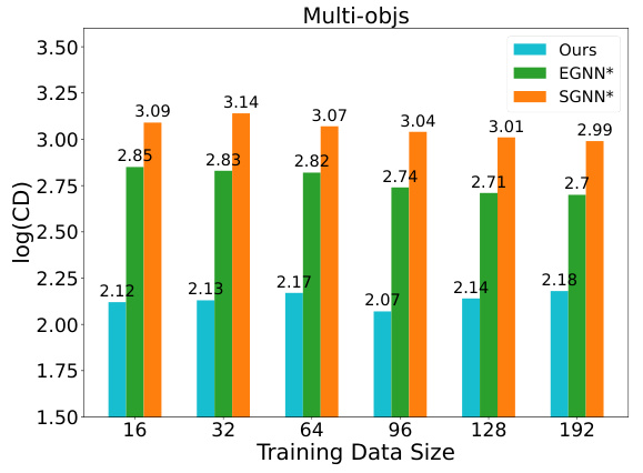
This paper is important because it presents a novel approach to learning 3D particle dynamics from 2D images, a challenging problem in computer graphics and robotics. The physics-integrated neural network improves robustness and generalizability compared to existing methods. This opens avenues for more realistic simulations in various fields using limited data and easier data acquisition methods. The work also offers a mechanically interpretable framework, improving understanding and future development.
Visual Insights#

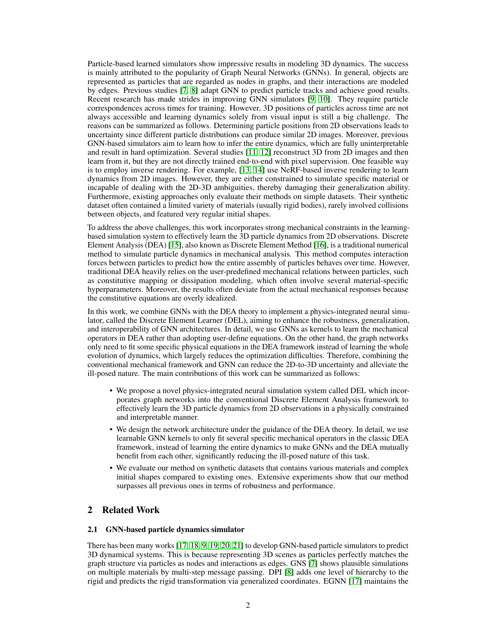
This figure illustrates the overall process of learning dynamics via inverse rendering. The left part (a) shows the initialization stage where a scene is represented as particles. The right part (b) illustrates the recurrent dynamic inference process. The system iteratively generates the particle sets and feeds them into a dynamic predictor to estimate their next states. The generated particles are rendered into images, and the errors between the rendered images and the ground truth images are used to train the model.

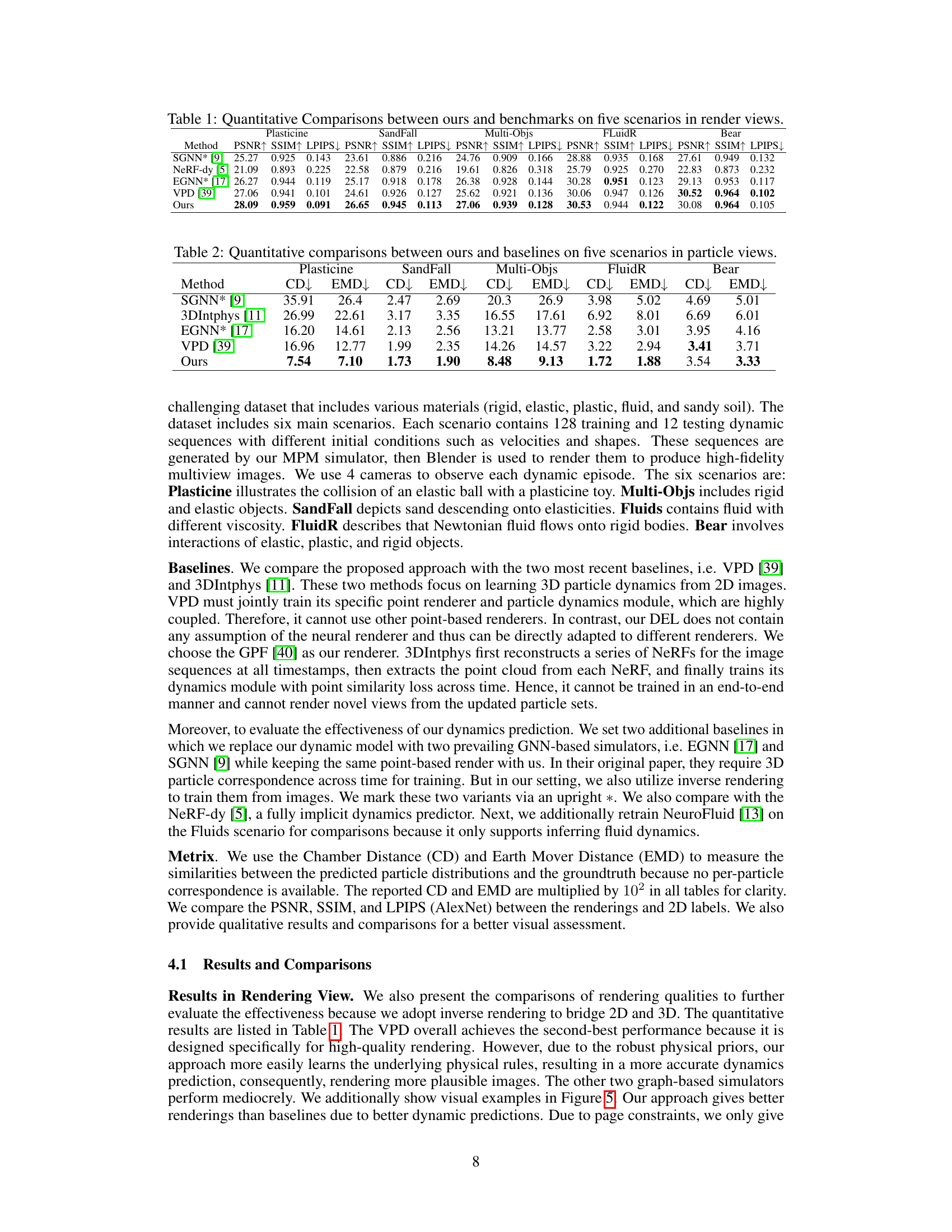
This table presents a quantitative comparison of the proposed method against several benchmark methods across five different scenarios, evaluating performance using PSNR, SSIM, and LPIPS metrics in render views. Higher PSNR and SSIM values, and lower LPIPS values indicate better performance. The scenarios likely involve different types of material interactions and object dynamics.
In-depth insights#
Physics-Integrated GNN#
A Physics-Integrated GNN represents a powerful paradigm shift in applying Graph Neural Networks (GNNs) to physical simulations. By directly incorporating physical laws and principles into the GNN architecture, it moves beyond simply learning empirical relationships between inputs and outputs. This integration could manifest in several ways, such as using physically-interpretable kernels, encoding physical properties as node features, or incorporating differentiable physics engines within the GNN framework. The key advantage lies in improved accuracy, generalization, and explainability. The model becomes less prone to overfitting, particularly when dealing with limited training data or complex scenarios, because the physical constraints guide the learning process. The interpretability of a Physics-Integrated GNN is a significant benefit, allowing researchers to gain a deeper understanding of the underlying physics rather than viewing the simulation as a black box. However, challenges remain. Designing efficient and effective ways to integrate physics into the GNN architecture can be complex, and finding the right balance between data-driven learning and physics-based modeling is crucial. Successfully addressing these challenges would lead to more robust and reliable simulations across a wide range of physical systems, with applications spanning robotics, materials science, and computational fluid dynamics.
Inverse Rendering#
Inverse rendering, in the context of this research paper, is a crucial technique for learning 3D particle dynamics from 2D image observations. It tackles the challenge of inferring complex 3D information (particle positions and interactions) from limited 2D projections. The core idea is to use a differentiable rendering process to bridge the gap between the 2D observations and the underlying 3D physical world. By minimizing the difference between rendered images (from simulated 3D particle states) and actual images, the model learns to predict the 3D dynamics accurately. This inverse process inherently addresses the ill-posed nature of recovering 3D information from 2D data, which is a major problem in this field. The success of this approach depends heavily on the choice of differentiable renderer, as it directly impacts the quality and informativeness of the rendered images. This method’s effectiveness is highlighted by its ability to achieve impressive results despite inherent ambiguities and the scarcity of data; however, its reliance on a suitable differentiable renderer presents a limitation.
Robustness & Limits#
A robust system should reliably perform its intended function across various conditions and inputs. This research paper, focusing on simulating 3D particle dynamics from 2D observations, would benefit from a dedicated ‘Robustness & Limits’ section. It should explore the model’s performance under various conditions, including diverse materials, limited training data, varied camera views, and noisy inputs. Key limitations would include the generalization capabilities to unseen scenarios, the assumptions underlying the physical model and its accuracy in representing real-world phenomena. Assessing robustness requires a thorough analysis of the model’s performance across different environments, exploring the effects of noise and variations to the inputs. This should encompass quantifiable metrics such as accuracy, precision and computational efficiency. The results should also consider potential edge cases and failure modes, identifying scenarios where the model might perform poorly or fail completely. The discussion of limits should be transparent, including challenges in representing complex physical interactions or limitations imposed by the chosen neural network architecture and training methods. The section should also provide suggestions for future research directions, such as improving robustness or extending the capabilities of the model. A comprehensive robustness analysis is crucial for building trust and reliability in the model’s predictions and its potential applications.
Material Diversity#
A crucial aspect of physically-realistic simulation is the ability to handle diverse materials. Material diversity in a particle-based simulator necessitates the capacity to model varied material properties such as elasticity, plasticity, viscosity, and friction. This demands a robust and flexible framework capable of representing these different behaviors. A successful approach would likely involve either learning material-specific parameters or employing a more general model that can adapt to a wide range of material characteristics. Learned parameters might involve using neural networks to represent constitutive models for different materials. This would require sufficient training data. Alternatively, a physics-informed approach, possibly incorporating a graph neural network structure informed by physics principles like Discrete Element Analysis (DEA), offers the advantage of generalizability. Such a framework may learn some material-specific features through the parameters of the network but still rely on the underlying physics, thus reducing the required data. A combination of these techniques could prove particularly effective, allowing for both efficient learning of material-specific details and leveraging of physics-based priors to improve generalization. Evaluated performance should be assessed on datasets containing materials with highly varied properties and across diverse interaction scenarios.
Future of DEL#
The future of DEL (Discrete Element Learner) is promising, particularly given its demonstrated ability to learn 3D particle dynamics from limited 2D observations. Further research should focus on enhancing the model’s robustness and generalizability by exploring alternative neural network architectures and incorporating more sophisticated physical priors. Investigating more complex scenarios involving diverse materials and interactions, such as those present in real-world settings, is crucial. Expanding the framework to handle larger-scale simulations and improving efficiency will be vital for practical applications. Extending DEL to different types of physical phenomena, beyond particle dynamics, offers significant potential. Addressing current limitations regarding non-Newtonian fluids and the simulation of materials like smoke is essential. Ultimately, the success of DEL hinges on its ability to seamlessly integrate with other advanced techniques in computer vision and simulation, bridging the gap between synthetic and real-world datasets for more realistic and accurate physical modeling.
More visual insights#
More on figures
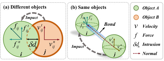
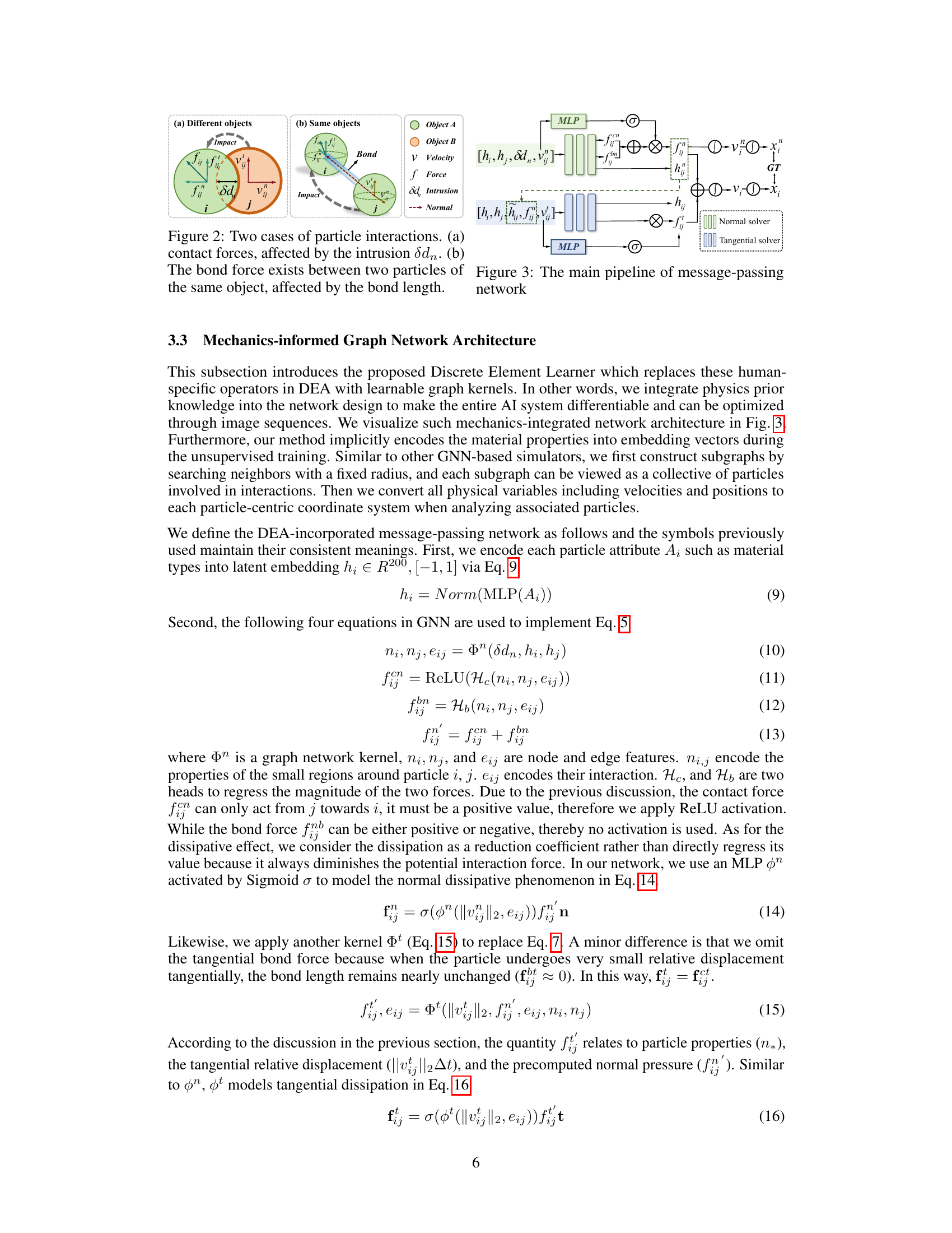
This figure illustrates two scenarios of particle interactions in the context of the Discrete Element Analysis (DEA) framework. Panel (a) shows the impact between two particles belonging to different objects. The forces involved are the contact force (fij) which has a normal component (fijn) and a tangential component (fijt), and the intrusion scalar (δdn) that measures the depth of interpenetration. Panel (b) depicts two particles belonging to the same object, connected by a bond. This bond force (fij) maintains the integrity and structure of the object. The interaction forces are determined by physical quantities like the intrusion scalar (δdn) and the bond length.
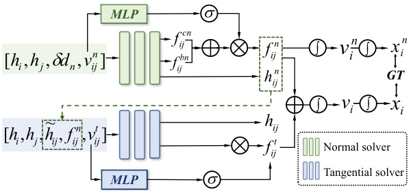
This figure shows the architecture of the mechanics-informed graph network used in the Discrete Element Learner (DEL). The network takes as input the node features [hi, hj] (particle attributes), edge features (δdn, vij) (intrusion and relative velocity), and then processes them through a series of learnable graph kernel operations (Φn, Φt) to produce the magnitudes of normal and tangential forces (fij, fij). These forces are then used to update particle velocities and positions, which are compared to ground truth (GT). The network consists of two branches: one for normal forces and one for tangential forces, each employing multiple MLP layers and ReLU activation functions. The network is designed to incorporate physical knowledge from the Discrete Element Analysis framework.

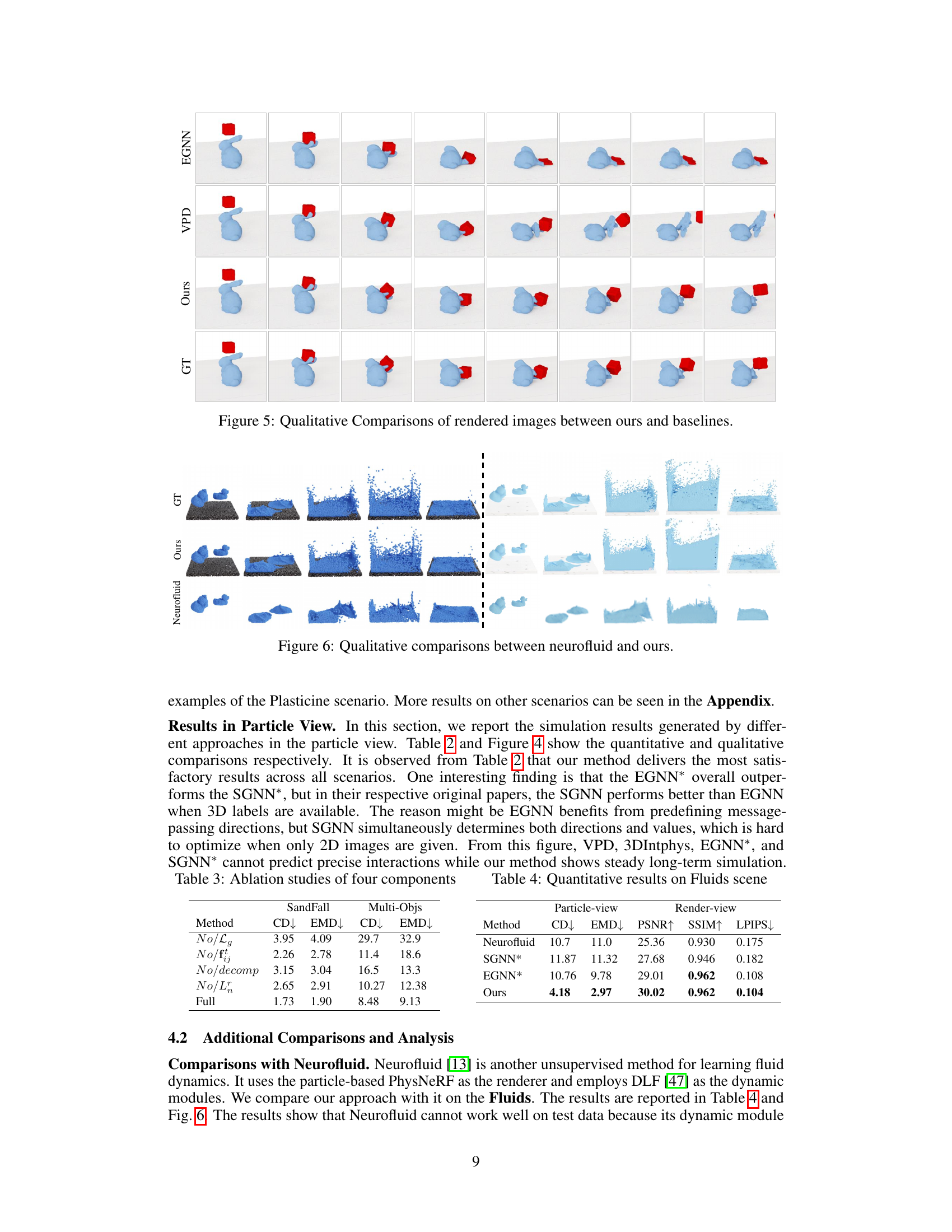
This figure shows a qualitative comparison of the dynamics prediction results of the proposed DEL method and several baseline methods. The comparison is shown in the particle view for test sequences. The figure visually demonstrates the superior performance of DEL in accurately predicting particle dynamics compared to the baselines. Each row represents a different method, and each column represents a different frame in the sequence.

This figure shows a qualitative comparison of the dynamics prediction results between the proposed DEL method and several baseline methods. The comparison is done in the particle-view, showing the predicted particle positions over time for a test sequence. It visually demonstrates the superior performance of DEL compared to baselines in accurately predicting the dynamics of the particles.

This figure presents a qualitative comparison of the results obtained using the proposed method and Neurofluid, another unsupervised method for learning fluid dynamics. The comparison shows the superior performance of the proposed method in accurately predicting the fluid dynamics, particularly in terms of the fluid’s shape and interaction with the rigid body, unlike Neurofluid which struggles with the overall flow and shape of the fluid.

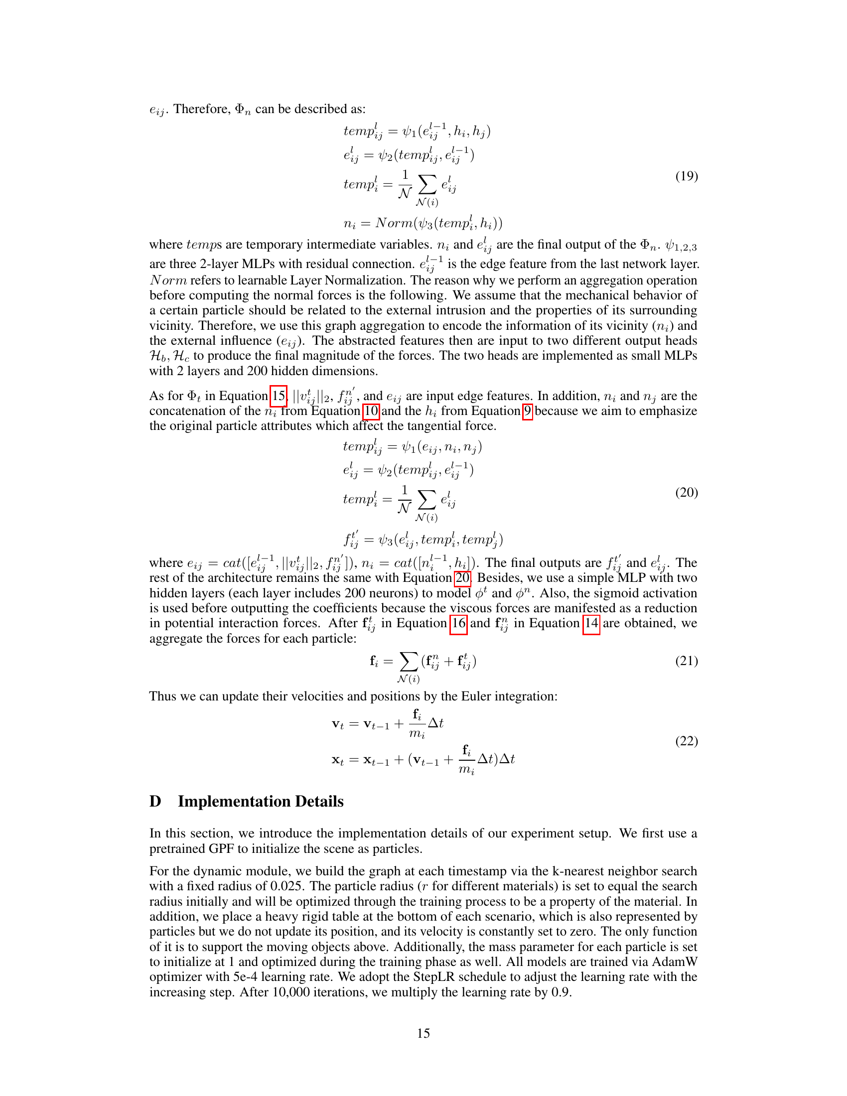
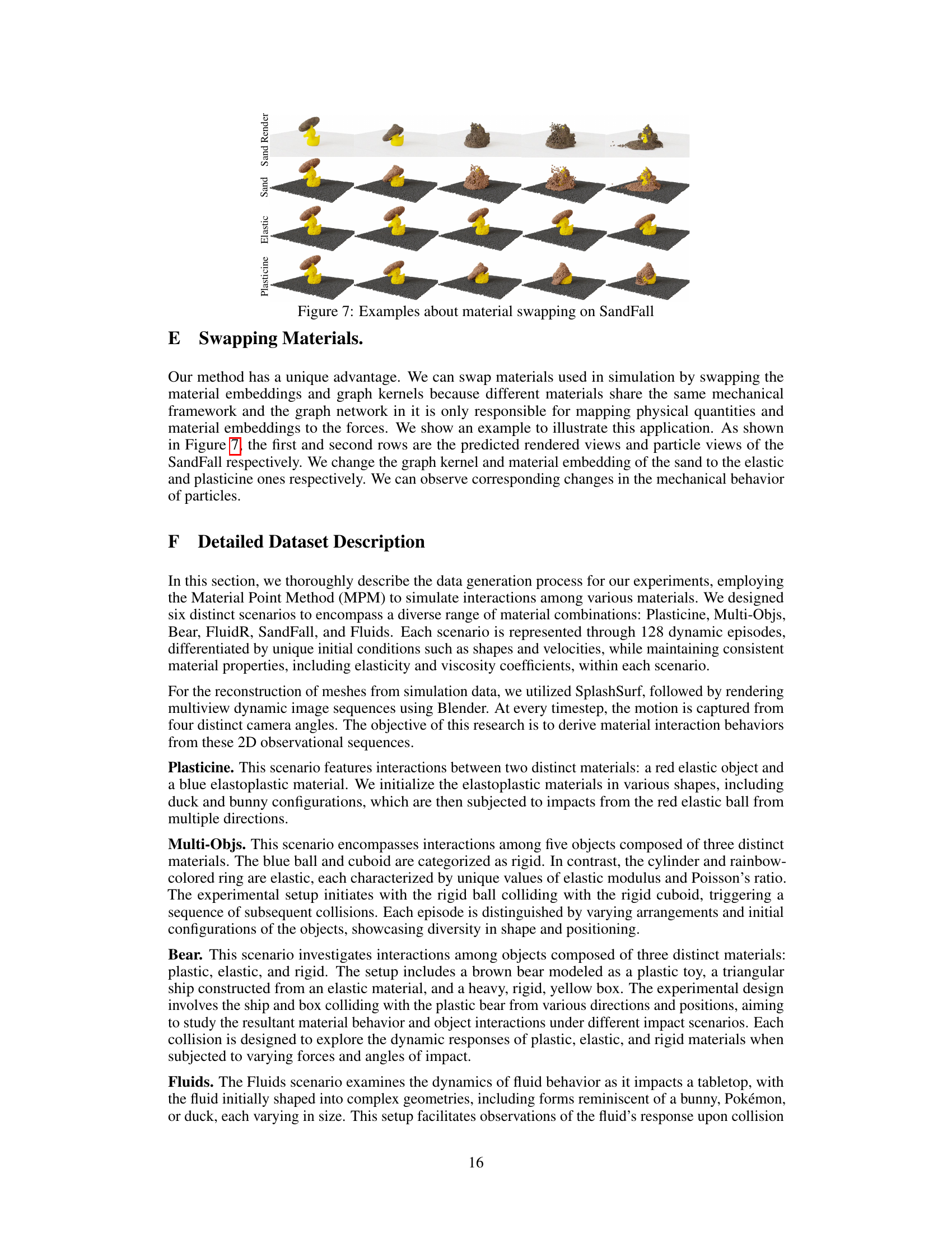
This figure demonstrates the capability of the DEL model to simulate different materials by simply swapping material embeddings and graph kernels. The top row shows the SandRender (rendered image) results of dropping a brown object onto a yellow duck on a sandy surface for different materials: Sand, Elastic, and Plasticine. The bottom three rows show the corresponding Sand results with the same parameters for each material.
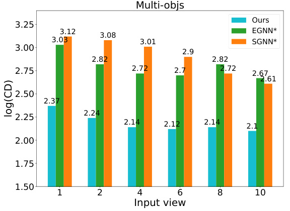
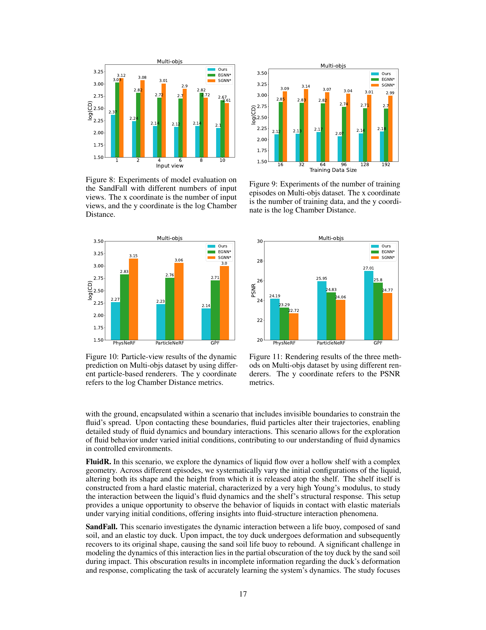
This figure shows the results of an experiment evaluating the performance of a model on the SandFall dataset using different numbers of input views. The x-axis represents the number of input views, while the y-axis shows the log of the Chamber Distance, a metric used to measure the similarity between the predicted particle distributions and the ground truth. The figure likely demonstrates how the model’s accuracy is affected by the number of camera views used during training, with more views potentially improving accuracy.
The figure shows the results of evaluating a model’s performance on the SandFall dataset using different numbers of input views. The x-axis represents the number of input views, and the y-axis represents the log Chamber Distance, which measures the similarity between predicted and ground truth particle distributions. It shows how the model’s accuracy changes as the number of input views increases.
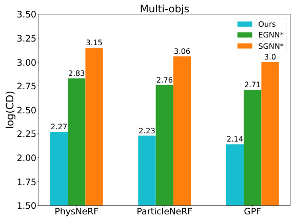
The bar chart compares the performance of three different particle-based renderers (PhysNeRF, ParticleNeRF, and GPF) in predicting the dynamics of the Multi-objs scenario in a particle view. The y-axis represents the log of the Chamber Distance, a metric used to evaluate the accuracy of particle distribution prediction. The chart shows that GPF outperforms the other two methods, indicating that the choice of renderer significantly impacts the results.
This figure compares the performance of different particle-based renderers (PhysNeRF, ParticleNeRF, and GPF) on the Multi-Objs dataset when predicting particle dynamics. The y-axis shows the log Chamber Distance, a metric used to evaluate the accuracy of the predicted particle distribution. The results show that the proposed method (Ours) outperforms the baselines regardless of the renderer used.

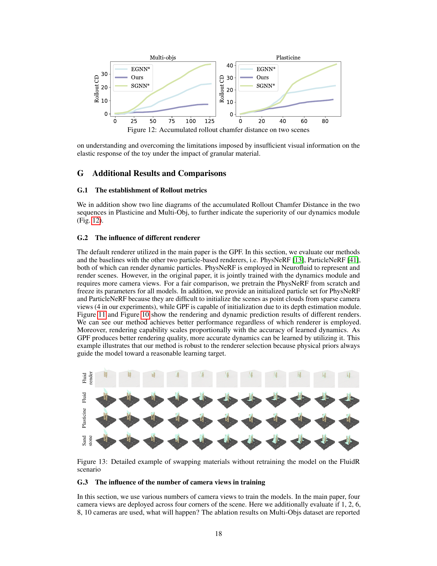
The figure shows the accumulated rollout chamfer distance over time for three different methods (EGNN*, Ours, SGNN*) on two scenarios: Multi-objs and Plasticine. It compares the performance of the proposed method against two baseline GNN-based simulators, highlighting the superior performance of the proposed approach in accurately predicting long-term dynamics. The x-axis represents the timestep and the y-axis represents the accumulated rollout chamfer distance, a metric measuring the difference between the predicted and ground truth particle positions.

This figure demonstrates the impact of swapping materials in the SandFall scenario. By replacing the material embeddings and graph kernels, the model adapts to different material properties. The first and second rows showcase the predicted views (rendering and particle views) of SandFall with sand, while the third and fourth rows depict the predictions after swapping the sand with elastic and plasticine materials, respectively. This highlights the flexibility and adaptability of the proposed model in handling diverse material interactions.

This figure shows how the model can handle material swapping by simply changing the material embedding and graph kernel. The top row displays the rendered views of a simulation where a yellow object falls onto sand. The second row shows the corresponding particle view. The third and fourth rows repeat the experiment, but with the sand replaced by plasticine and elastic materials, respectively. The results demonstrate the model’s adaptability to different material properties.

This figure shows a visualization of removing the bond force from the simulation. The left side shows the input, a red object impacting a blue object on a gray surface. The right side shows the multi-view simulation results with the bond force removed, highlighting how the lack of bond force affects the interaction and shape of the objects during the impact.

This figure visualizes the impact of removing the bond force from the simulation. The left side shows the input (initial state) and the simulation result when the bond force is included. The right side shows the multi-view simulation result when the bond force is removed. This illustrates the effect the bond force has on maintaining the structural integrity of the simulated objects. Without it, the simulated objects show significant structural deviations.
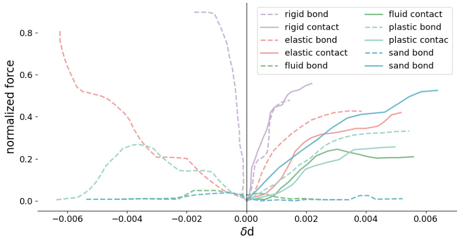
This figure visualizes the learned constitutive mapping, a key component of the Discrete Element Learner (DEL) model. The x-axis represents the intrusion (δd), a measure of how much one particle penetrates another. The y-axis shows the normalized force magnitude. Different colored lines represent different material pairings (e.g., rigid bond, rigid contact, elastic bond, etc.). The plot shows how the model learns to associate different levels of intrusion with different force magnitudes for various material types, demonstrating the model’s ability to capture material-specific mechanical behavior.
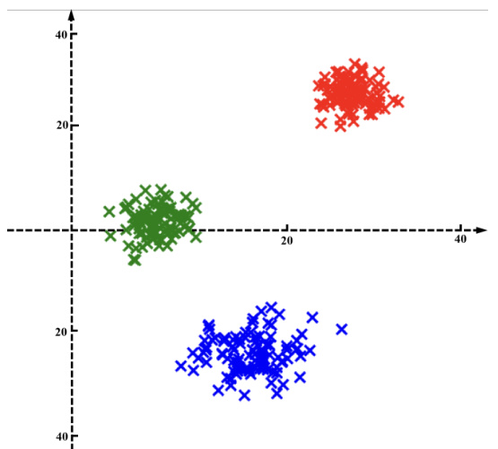
This figure visualizes the learned material embeddings using t-SNE. Different colors represent different materials (red for rigid, green and blue for two types of elastic materials). Points from the same object cluster together, demonstrating that the model has learned material-specific features. The spatial relationships of points within each cluster reflect their positions relative to the center of mass of the object, further enhancing the model’s understanding of material properties in context.
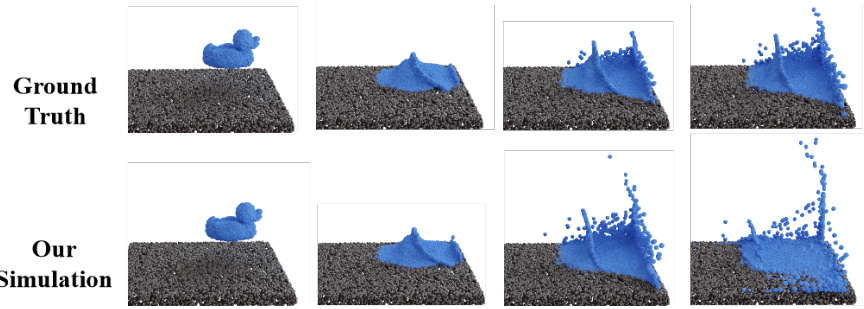
This figure displays a qualitative comparison of the dynamics prediction results of the proposed method (DEL) against several baseline methods. The comparison is shown in terms of particle-view visualizations on test sequences. This allows for a visual assessment of the accuracy and robustness of the different methods in predicting the motion of particles over time.
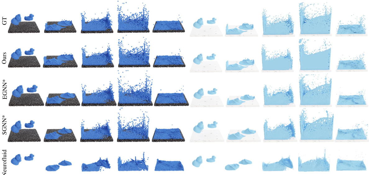
This figure presents a qualitative comparison of the proposed DEL model against several baselines (3DIntphys, VPD, EGNN*, SGNN*, and Neurofluid) for the Fluids dataset. The comparison includes both rendering (top row) and particle views (bottom row) across multiple time steps of the simulation. The goal is to visually demonstrate the relative performance of each method in simulating fluid behavior.
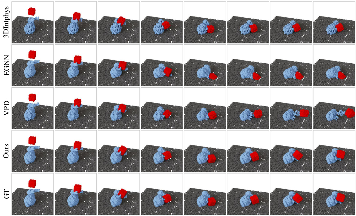
This figure shows a qualitative comparison of the dynamics prediction results from different methods, including the proposed DEL and other baseline methods. The comparison is made on test sequences in the particle view. The figure aims to visually demonstrate the performance difference of DEL and baselines for better understanding.
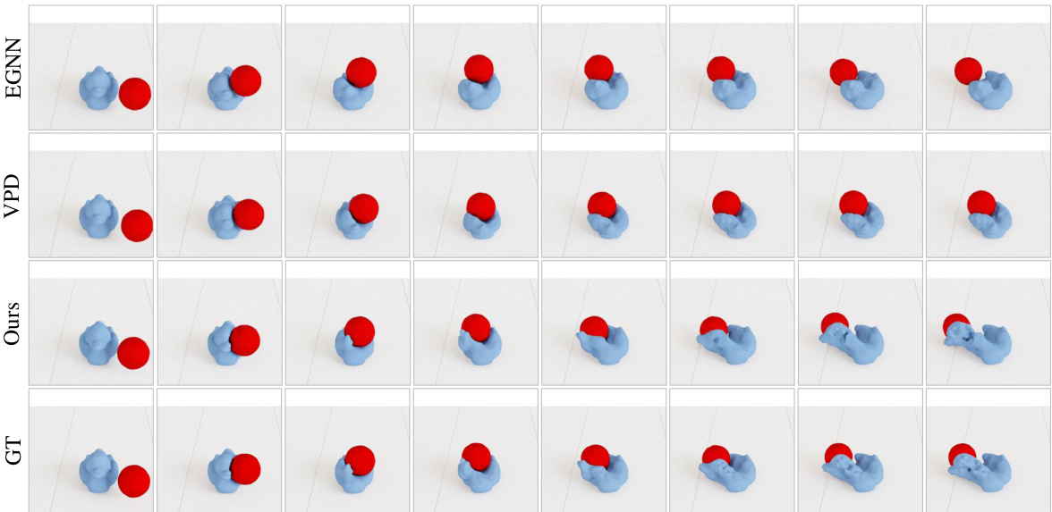
This figure shows a qualitative comparison of the dynamics prediction results between the proposed method (DEL) and several baseline methods. The comparison is done in the particle view on test sequences. The figure visually demonstrates the superior performance of DEL in accurately predicting the dynamic behavior of particles compared to the baselines. It highlights DEL’s ability to handle complex interactions and various material properties.
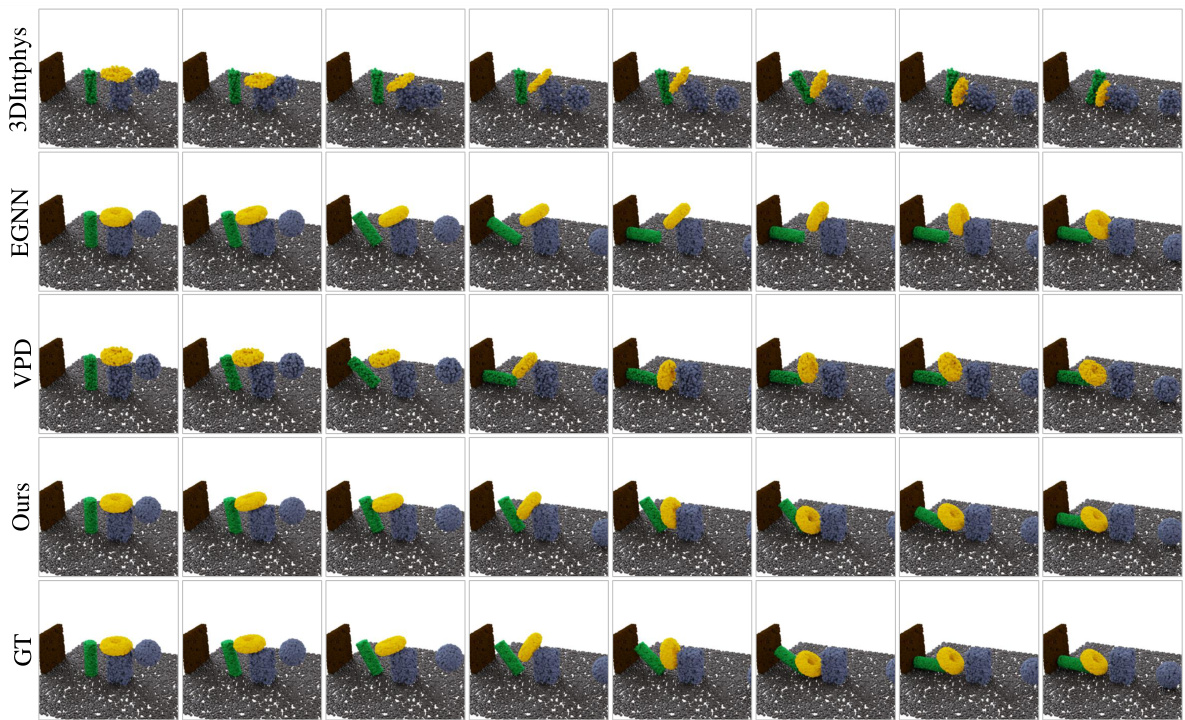
This figure provides a qualitative comparison of the dynamics prediction results from the proposed DEL method and other baseline methods. The comparison is shown in the particle-view for test sequences. It allows for visual inspection of how well each method captures the movement and interactions of particles in a dynamic scene. This visual comparison is useful to assess the accuracy and realism of each method’s predictions, especially concerning the overall movement and interactions of particles.
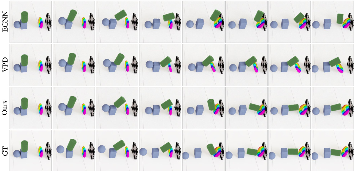
This figure presents a qualitative comparison of the dynamics prediction results obtained using the proposed DEL method and several baseline methods. The comparison is shown in the particle-view for test sequences. Each row represents a different method (GT, Ours, VPD, EGNN, 3DIntphys), and each column shows the simulation results at different time steps. This allows for a visual assessment of the accuracy and realism of the different methods in predicting the motion of particles over time.

This figure shows a qualitative comparison of the dynamics prediction results of the proposed DEL method and several baseline methods on test sequences. The comparison is shown in the particle view. The figure visually demonstrates the performance of DEL compared to baselines in accurately predicting particle movements over time. It highlights the superior performance of DEL in capturing the complex dynamics of particle interactions.
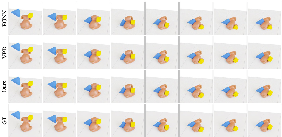
This figure presents a qualitative comparison of dynamics prediction results between the proposed DEL method and several baseline methods. The comparison focuses on the particle-view perspective of test sequences. It visually demonstrates the differences in the accuracy and realism of the simulated particle dynamics generated by each method. The figure aids in assessing the performance and robustness of DEL against existing techniques in handling complex 3D particle dynamics.
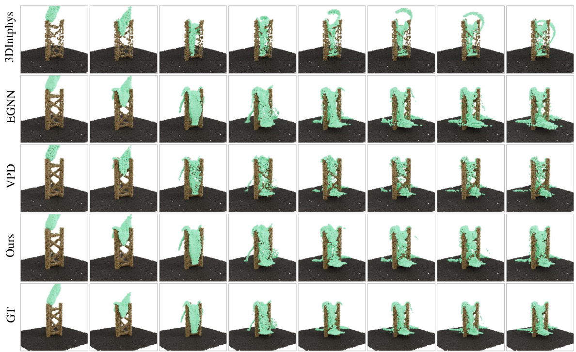
This figure compares the long-term predictions of four different methods (3DIntphys, VPD, EGNN, and the proposed method) on the FluidR scenario. The predictions are shown in particle view, allowing visualization of the individual particles’ movements over time. The ground truth (GT) is included for comparison. The figure visually demonstrates the relative accuracy and robustness of each method in simulating the fluid’s behavior over an extended time period.
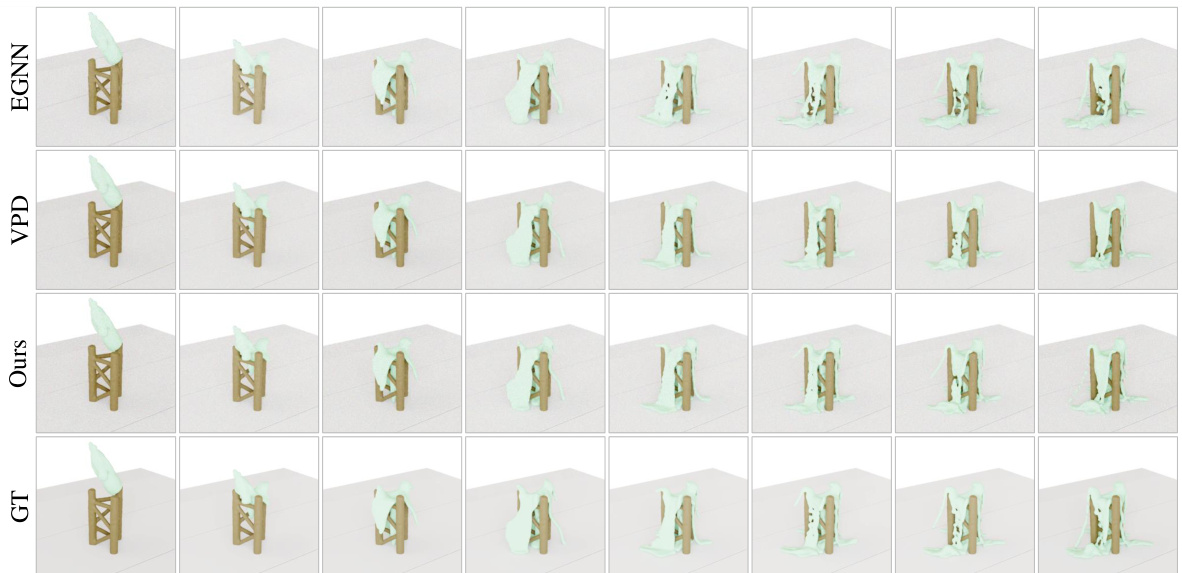
This figure presents a qualitative comparison of the dynamics prediction results obtained using the proposed DEL method and several baseline methods. The comparison focuses on the particle view, showing the predicted particle positions over time for different methods. The goal is to visually demonstrate the superior performance of DEL in accurately predicting the dynamics compared to the baselines.
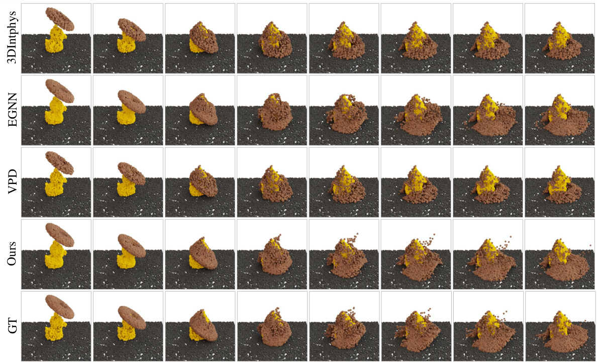
This figure shows a qualitative comparison of the dynamics prediction results between the proposed DEL method and several baseline methods. The comparison is shown in a particle-view perspective for test sequences. It allows a visual assessment of the accuracy and robustness of different methods in predicting particle movements and interactions over time.
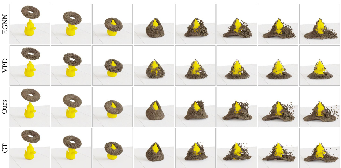
This figure presents a qualitative comparison of the dynamics prediction results obtained using the proposed DEL method and several baseline methods. The comparison is done in the particle view for test sequences. It visually demonstrates the differences in the accuracy and realism of the dynamics predictions generated by each method. The results highlight the superior performance of the DEL method in accurately capturing and simulating the complex dynamics of various materials and interactions.
More on tables

This table presents a quantitative comparison of the proposed method against existing baselines (SGNN, 3DIntphys, EGNN, VPD) across five different scenarios (Plasticine, SandFall, Multi-Objs, FluidR, Bear) in terms of particle-level accuracy. The metrics used are Chamfer Distance (CD) and Earth Mover’s Distance (EMD), both lower is better, reflecting the difference between the predicted and ground truth particle distributions.
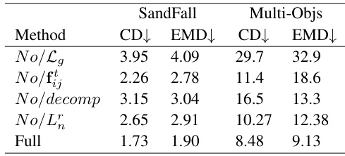
This table presents the ablation study results for four components of the proposed DEL model. It shows the impact of removing or altering the gradient loss (Lg), the tangential force (fij), the decomposition of the graph network, and the normal direction loss (Ln) on the performance of the model. The results are measured using Chamber Distance (CD) and Earth Mover Distance (EMD) metrics for two scenarios: SandFall and Multi-Objs.
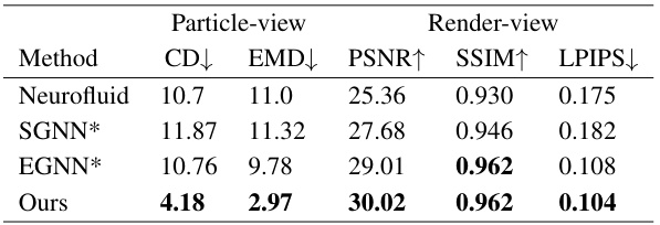
This table presents a quantitative comparison of different methods on the Fluids scene. The metrics used are Chamber Distance (CD), Earth Mover Distance (EMD), Peak Signal-to-Noise Ratio (PSNR), Structural Similarity Index (SSIM), and Learned Perceptual Image Patch Similarity (LPIPS). Lower CD and EMD values indicate better performance, while higher PSNR and SSIM and lower LPIPS values also indicate better performance.
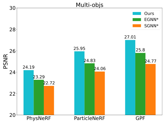
This table presents a quantitative comparison of the proposed method against several benchmark methods across five different scenarios. The comparison is based on metrics calculated from rendered images (PSNR, SSIM, and LPIPS). The scenarios represent diverse physics simulations involving various materials and object interactions. Higher PSNR and SSIM values, and lower LPIPS values indicate better performance.

This table presents a quantitative comparison of the proposed DEL method against several baseline methods across five different scenarios. The comparison is done using the Rollout Mean Squared Error (MSE) metric, which assesses the accuracy of dynamic predictions in particle views when 3D ground truth is available. Lower MSE values indicate better performance. The scenarios evaluated represent diverse physical interactions, including collisions of various materials and objects with different properties, such as Plasticine, SandFall, Multi-Objs, FluidR, Bear, and Fluids. The table allows for a direct comparison of the DEL’s performance relative to existing state-of-the-art methods under the condition of utilizing 3D ground truth data.
Full paper#
