↗ OpenReview ↗ NeurIPS Homepage ↗ Chat
TL;DR#
Many studies rely on randomized controlled trials (RCTs) for evaluating policies but face challenges in generalizing results to broader target populations which may differ systematically from the trial population. This paper focuses on making externally valid inferences using experimental data from RCTs combined with additional covariate data from the intended target population. It highlights the limitations of standard methods in achieving external validity, such as inverse probability weighting which may produce biased estimates when the sampling model is misspecified.
The paper proposes a novel, nonparametric policy evaluation method that uses a sampling model trained on the extra covariate data. This method is designed to give valid policy evaluations regardless of model miscalibration. The validity is assured using finite-sample guarantees. The paper also introduces a method to assess the credibility of the sampling model through benchmarking and demonstrates the performance of the proposed method using both simulated and real data from a seafood consumption study, highlighting the importance of the approach for safety-critical applications.
Key Takeaways#
Why does it matter?#
This paper is crucial for researchers seeking to improve the external validity of randomized controlled trials (RCTs). It offers a novel nonparametric method for evaluating policies using both RCT data and supplementary data from the target population. This approach directly addresses the challenge of generalizing RCT results to different populations, a significant issue in many fields. The paper also provides valuable guidance on assessing the credibility of the models used, promoting more reliable and trustworthy policy evaluation.
Visual Insights#

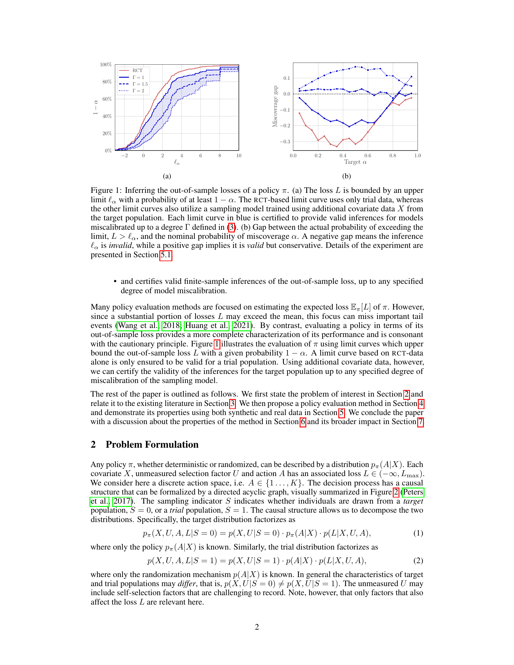
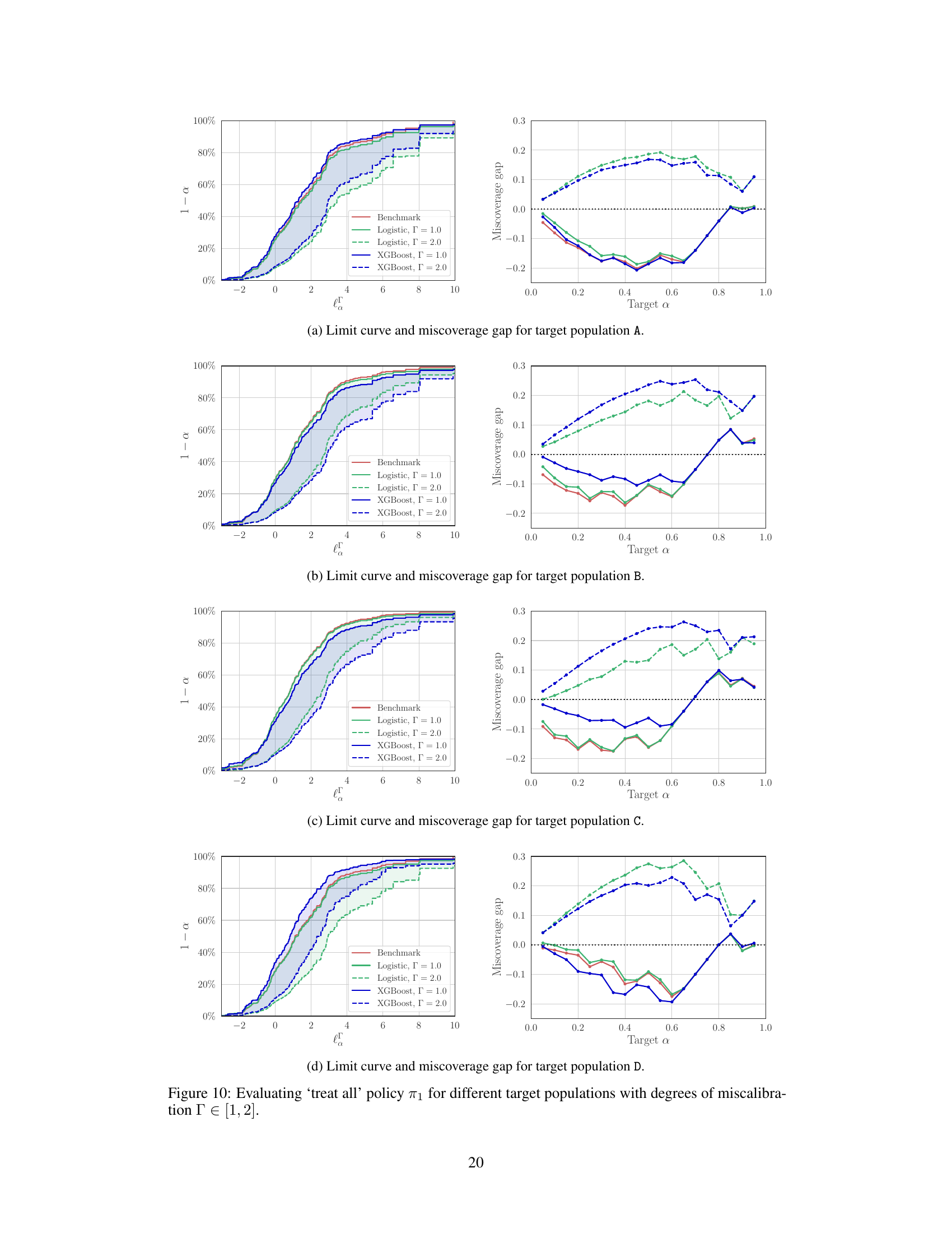
The figure shows how to infer the out-of-sample losses of a policy π using both trial data and additional covariate data from the target population. Subfigure (a) shows limit curves for different degrees of model miscalibration, demonstrating that the proposed method provides valid inferences even with miscalibrated models. Subfigure (b) shows the miscoverage gap, which is the difference between the actual probability of exceeding the limit and the nominal probability. A positive gap means that the inference is valid but conservative, while a negative gap indicates that the inference is invalid.

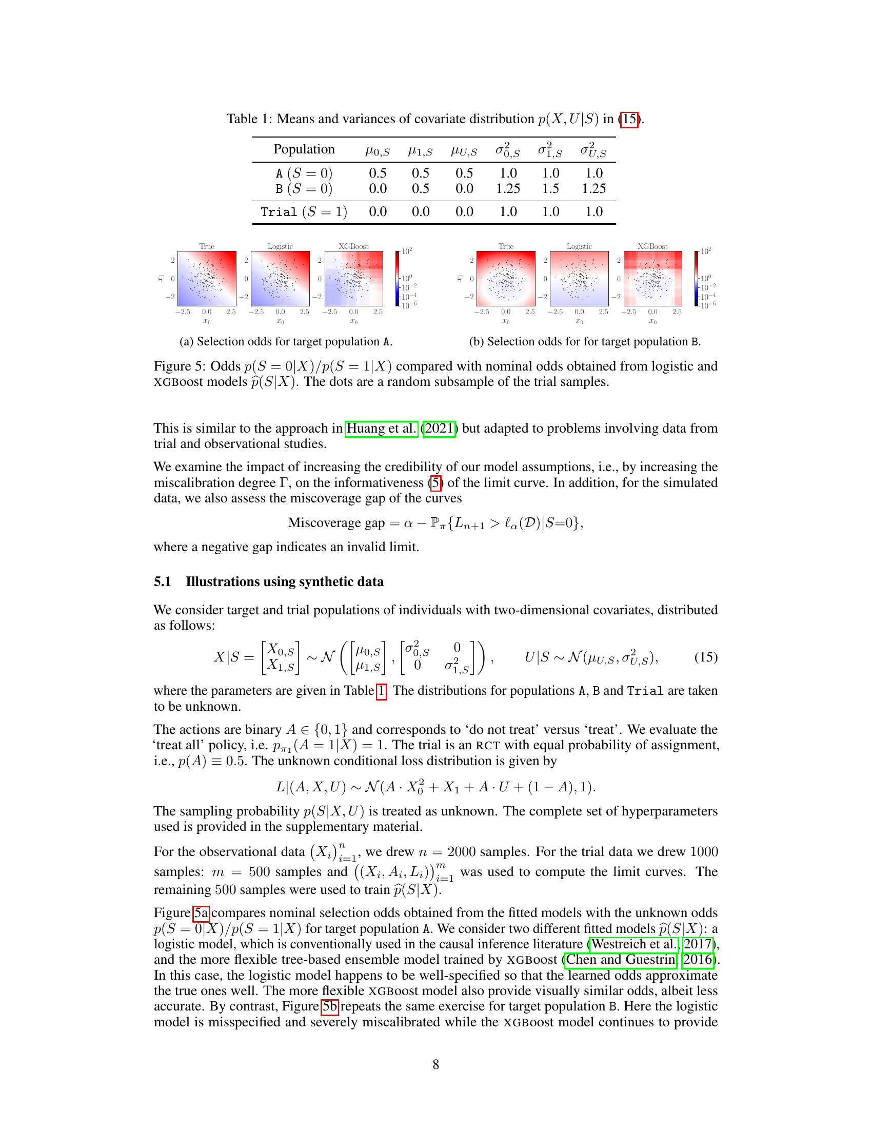
This table shows the means (μ) and variances (σ²) of the covariates X, U in the target populations (A, B) and the trial population. The data is drawn from a multivariate normal distribution N(μ, Σ), where μ represents the means and Σ the covariance matrix. The covariates X and U are used to model the sampling process (in Equation 15) and to calculate the odds ratio and loss.
In-depth insights#
Ext Validity RCTs#
Extending the validity of Randomized Controlled Trials (RCTs) is crucial for ensuring that research findings translate effectively to real-world settings. External validity, often referred to as generalizability, addresses the question of whether the causal inferences drawn from a specific RCT sample can be reliably applied to a broader target population. RCTs, while rigorous in their internal validity (ensuring causal effects are accurately measured within the study sample), may struggle with external validity due to limitations in sample selection and the presence of unmeasured confounding variables. Improving external validity often involves careful consideration of the sampling methodology, ensuring the sample is representative of the target population, and employing statistical techniques to account for potential biases. Sophisticated modeling approaches that incorporate covariate data from the target population can adjust for differences in the trial and target distributions. However, there’s no guarantee that these models are perfectly calibrated, which means evaluating the robustness of external validity to model misspecification is key. Sensitivity analyses are critical for determining how sensitive the RCT conclusions are to various degrees of model miscalibration, providing insights into the limits of generalizability.
Policy Evaluation#
Policy evaluation is a critical aspect of evidence-based decision-making. This paper focuses on enhancing the external validity of policy evaluations derived from randomized controlled trials (RCTs) by incorporating additional observational data from the target population. The core methodology addresses the issue of generalizability, a common challenge in RCTs where the trial population may not perfectly represent the intended target population. By leveraging supplementary covariate data, the approach aims to construct certifiably valid inferences about the policy’s impact on the target population even under model miscalibrations. This is achieved through a nonparametric method that provides finite-sample guarantees. The method’s robustness is highlighted by its ability to handle covariate shifts and unmeasured selection factors. Benchmarking techniques are incorporated to establish credible bounds for model miscalibration, improving the trustworthiness of the conclusions. Ultimately, the proposed method aims to bridge the gap between experimental results and real-world applications of policy interventions, improving the reliability and impact of decision-making.
Sampling Model#
The effectiveness of the proposed policy evaluation method hinges significantly on the accuracy of the sampling model, which aims to capture the relationship between the trial and target populations. A well-calibrated sampling model is crucial for valid inference, as miscalibration can lead to biased policy evaluations even with large sample sizes. The choice of model (logistic regression or more flexible models like XGBoost) impacts the model’s ability to capture complex relationships between covariates and selection bias. Benchmarking techniques that estimate the degree of model miscalibration (Γ) using omitted covariates are essential for establishing the credibility of inferences. By quantifying the potential range of miscalibration, researchers can assess the robustness of their policy evaluations and determine an appropriate level of conservatism, thereby ensuring the validity of inferences remains unaffected. However, model complexity necessitates a trade-off. While more complex models might capture nuanced relationships better, simpler models may have more credible calibration estimates for a given dataset, influencing the degree of miscalibration reported.
Certified Bounds#
The concept of “Certified Bounds” in a research paper likely refers to guaranteed or verifiable limits on a particular quantity, often related to uncertainty or variability in model predictions or experimental results. The “certified” aspect implies a high degree of confidence in these bounds, often achieved through rigorous mathematical proofs or statistical techniques that account for potential sources of error or uncertainty, such as finite sample sizes, model misspecification, or unobserved confounders. These bounds provide a measure of robustness and reliability, ensuring that conclusions drawn from the analysis remain valid even under certain levels of uncertainty. A focus on certified bounds is especially important in high-stakes settings where the consequences of incorrect inferences are severe (e.g., clinical decision-making). The paper likely uses a method to establish these bounds, accompanied by formal guarantees of validity. This would enhance the trustworthiness of the research and allow for more informed decision-making based on the findings.
Real-world Impact#
This research significantly impacts real-world policy evaluation by offering a robust, nonparametric method to extrapolate findings from randomized controlled trials (RCTs) to broader target populations. Its key strength lies in handling covariate shifts and model misspecifications, ensuring certified validity even with finite samples. This is particularly valuable in high-stakes domains like healthcare and safety-critical applications where cautious generalization is crucial. The method’s ability to certify the validity of inferences up to a specified degree of model miscalibration empowers decision-makers to make more informed and responsible choices. By focusing on out-of-sample loss, it moves beyond simple expected loss estimations, providing a more comprehensive understanding of policy effectiveness. The proposed benchmarking approach, further enhances practical applicability by providing guidelines for selecting appropriate miscalibration levels.
More visual insights#
More on figures
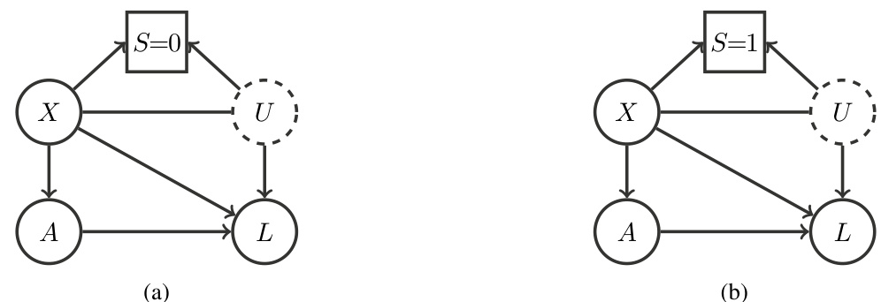
This figure shows the causal structure of the decision process under a policy (Figure 2(a)) and in a trial study (Figure 2(b)). The variable S is an indicator for whether the data comes from the target population (S=0) or the trial population (S=1). The figure shows the causal relationships between covariates X, unmeasured selection factors U, actions A, and losses L. The key difference between (a) and (b) is that in the RCT scenario (b), there is no direct causal link between the covariates X and the actions A.

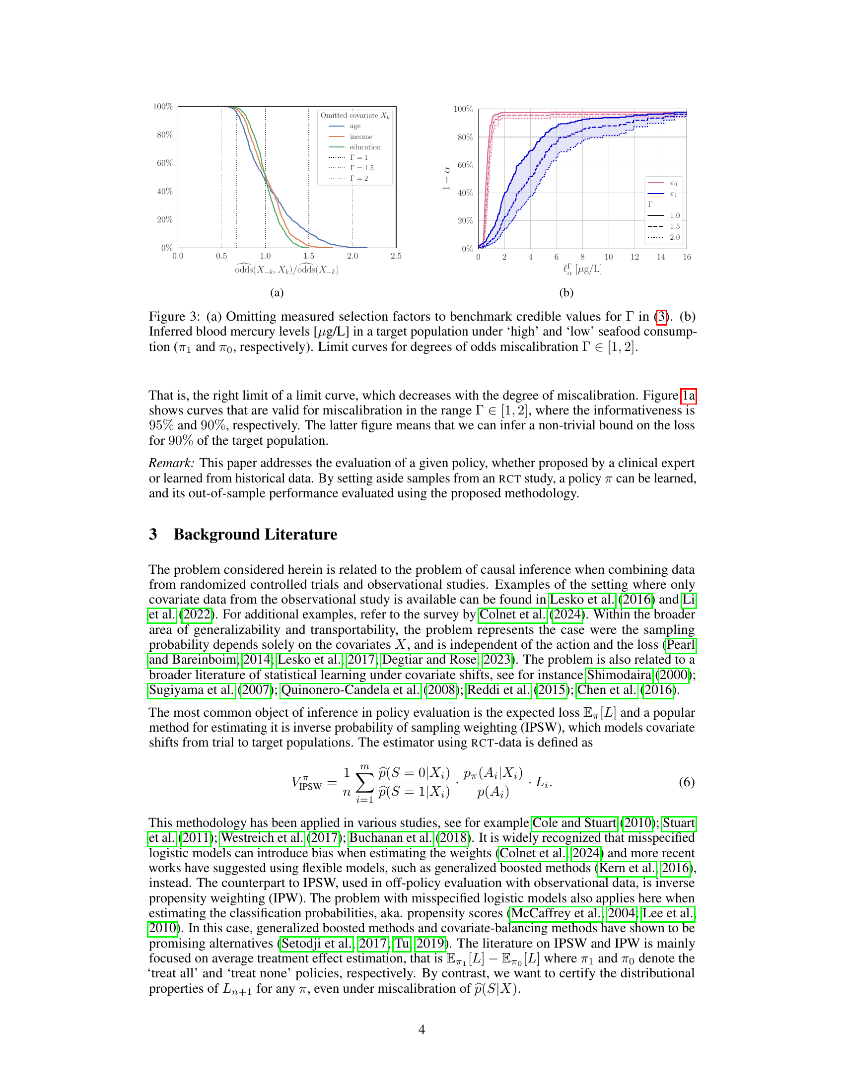
Figure 3(a) shows how omitting measured covariates (age, income, education) from the model of selection odds p(S|X) helps in establishing credible values for the parameter Γ, representing the degree of miscalibration. Figure 3(b) displays the inferred blood mercury levels for a target population based on different seafood consumption policies (‘high’ - π₁, ’low’ - πο). The limit curves, illustrating upper bounds for losses under these policies, are depicted for different levels of odds miscalibration (Γ = 1, 1.5, 2).

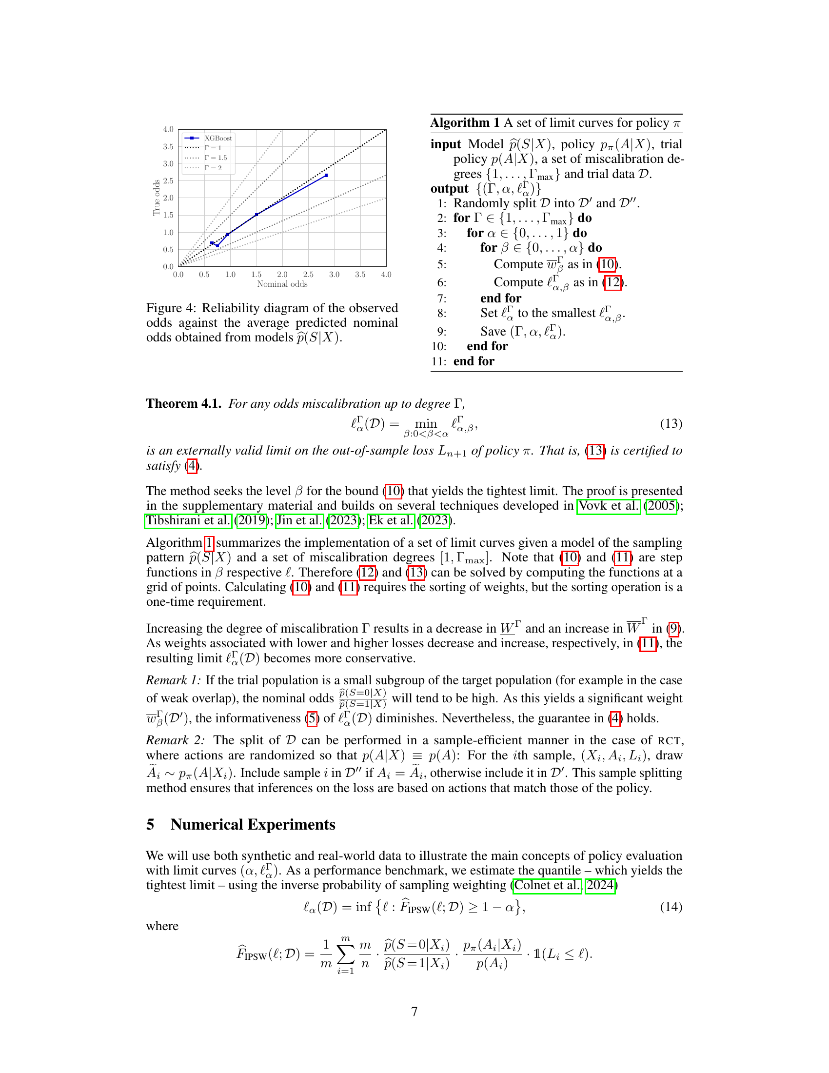
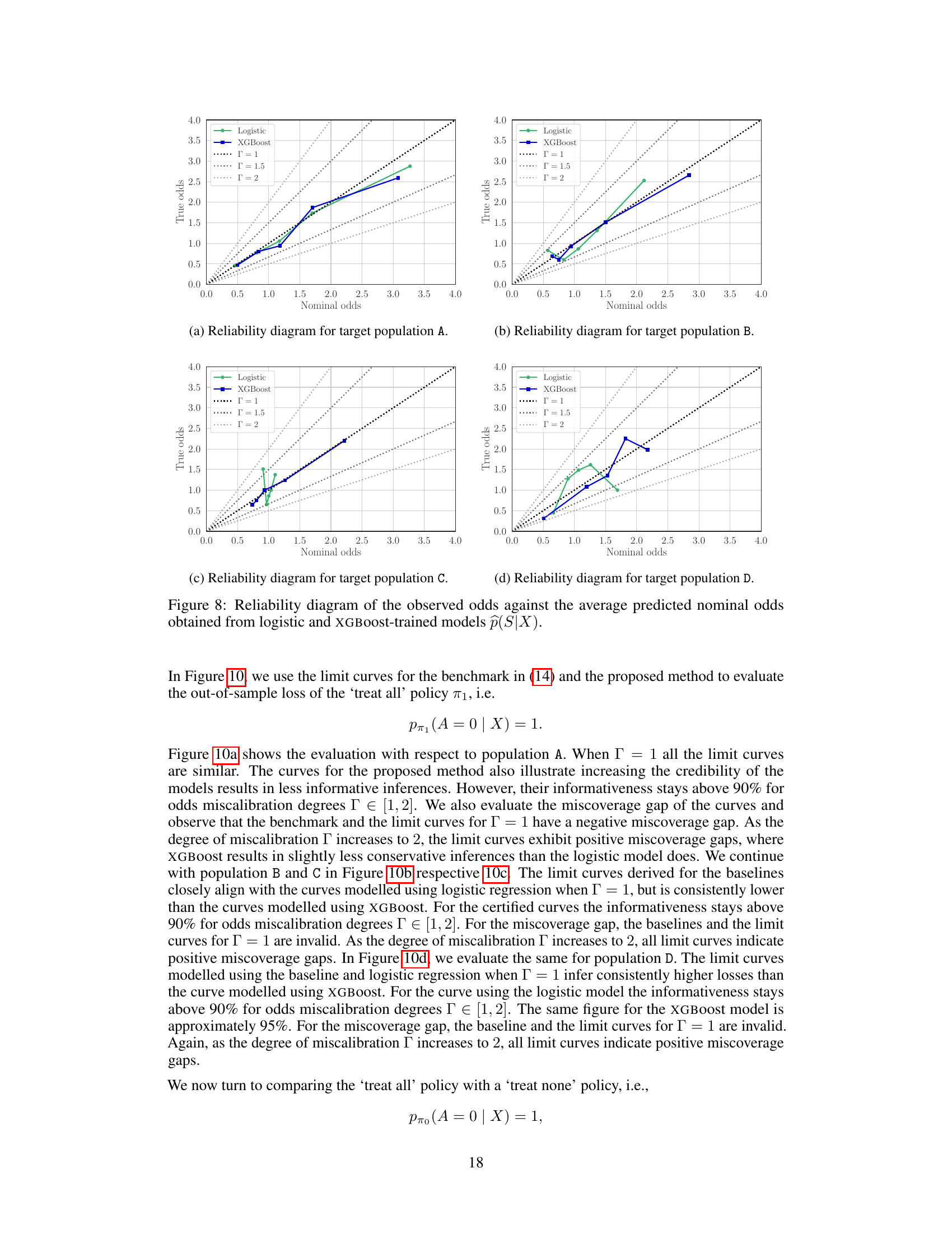
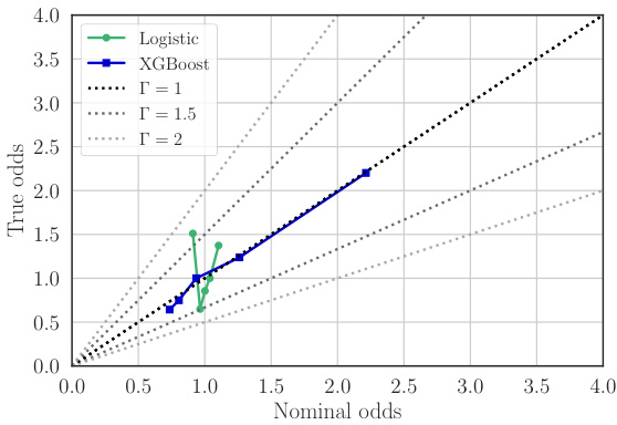
This figure shows a reliability diagram. A reliability diagram is a graphical way to assess the calibration of a predictive model, specifically focusing on how well predicted probabilities align with observed outcomes. The x-axis shows the average predicted probability (nominal odds), and the y-axis shows the average observed probability (true odds). A perfectly calibrated model would have all points lying along the diagonal line. Deviations from the diagonal indicate miscalibration. This diagram specifically examines the model p(S|X) used for estimating the probability of an individual being sampled from the target population (S=0) or trial population (S=1) given their covariates X. The plot shows results for XGBoost model, which appears reasonably well-calibrated.

This figure shows the results of an experiment to infer the out-of-sample losses of a policy. It compares the performance of using only randomized controlled trial (RCT) data versus also using additional covariate data from the target population and a sampling model. The plots show the upper bound of the loss with a given probability, along with the gap between the actual and nominal probabilities of exceeding that bound. This demonstrates the method’s ability to provide valid inferences even with miscalibrated models.

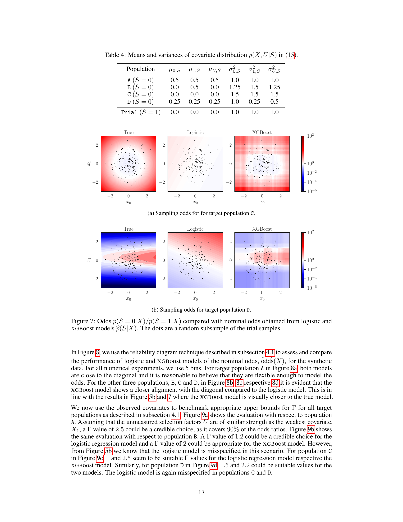
This figure compares the true selection odds (the ratio of the probability of being from the target population to the probability of being from the trial population, given covariates X) to the selection odds predicted by two different models: a logistic model and an XGBoost model. The heatmaps represent the estimated odds from each model. The dots show a random sample of points from the trial data. The purpose of the figure is to visually show how well the models capture the true selection odds. It demonstrates that the XGBoost model is a better fit for this specific dataset.

This figure compares the true odds of selection (p(S=0|X)/p(S=1|X)) with the odds predicted by two different models: a logistic model and an XGBoost model. The true odds represent the actual probability of an individual from the target population being sampled in the trial, given their covariates X. The predicted odds from the models aim to estimate these true odds. The plots visualize the results for two different target populations (A and B). Each subplot displays a heatmap showing the true odds (leftmost column) and the predicted odds from each model. The dots represent a random selection of the data from the trial population. The visual comparison helps assess the accuracy of the different models in predicting the true selection odds and can inform the level of potential model miscalibration (Γ).
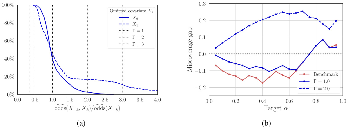
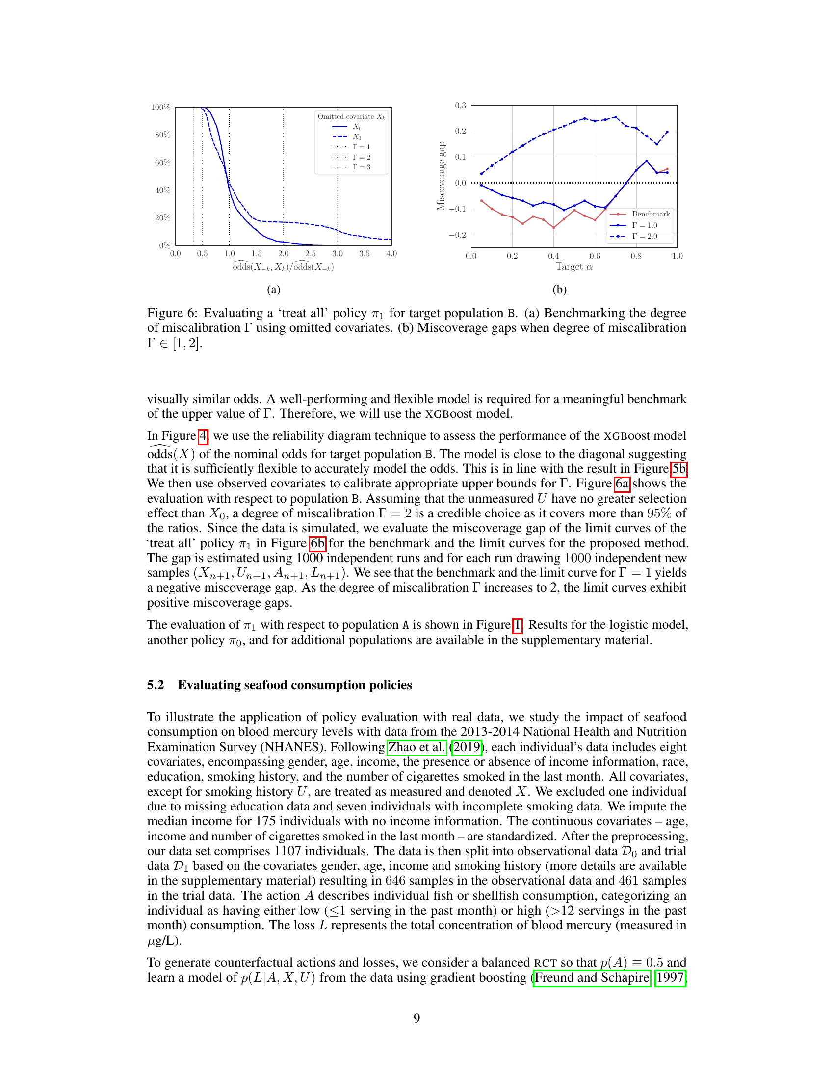
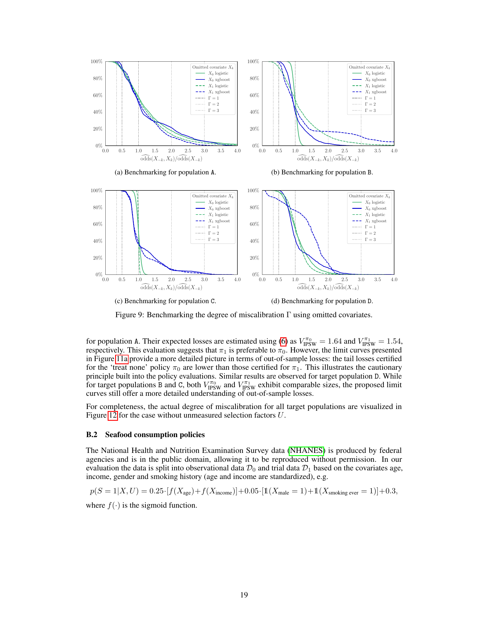
This figure shows the results of benchmarking the degree of miscalibration (Γ) for the ’treat all’ policy (π₁) applied to target population B. Panel (a) shows how the selection odds ratio changes when covariates are omitted, providing a benchmark to choose a reasonable Γ value. Panel (b) illustrates the miscoverage gap – the difference between the nominal and actual probability of exceeding a loss limit (lα) – for different Γ values and nominal probabilities (α). A positive gap indicates a valid, but conservative, inference; a negative gap signifies an invalid inference. This analysis helps determine the credibility of the policy evaluation under varying degrees of model miscalibration.
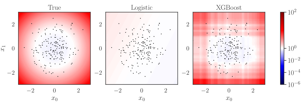
This figure compares the true selection odds (the ratio of probabilities of being in the target population given covariates X) with the selection odds predicted by logistic and XGBoost models. It helps to assess the quality of the sampling model used in the proposed method. The dots represent a random sample from the trial data, providing a visual comparison of the model predictions against the true ratios.

This figure compares the true selection odds, p(S=0|X)/p(S=1|X), with the selection odds predicted by a logistic regression model and an XGBoost model. The true odds represent the ratio of the probability of observing a sample from the target population to the probability of observing a sample from the trial population, conditional on the covariates X. The logistic and XGBoost models are trained on the trial data to estimate this ratio. The dots represent a random subsample of the trial samples. The visualization helps assess the accuracy and calibration of the models in estimating the selection odds, which is crucial for the proposed policy evaluation method.
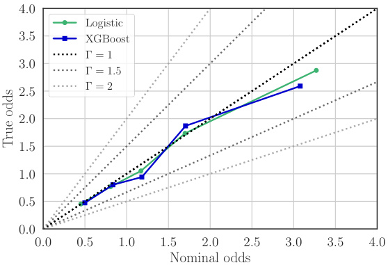
Figure 3(a) shows how omitting certain measured selection factors from the model can help determine credible values for the parameter Γ, which represents the degree of odds miscalibration in the model. Figure 3(b) displays the inferred blood mercury levels in a target population under two different seafood consumption policies, ‘high’ and ’low’, represented by π₁ and πο respectively. The figure includes limit curves illustrating the uncertainty associated with varying degrees of model miscalibration (Γ values between 1 and 2).

This figure shows the reliability of the models used to estimate the selection odds p(S|X). A well-calibrated model should have points close to the diagonal line. The plot suggests that the XGBoost model is better calibrated than the logistic model, especially in the higher ranges of nominal odds, where the logistic model underestimates the true odds.
This figure shows how to benchmark credible values for the parameter Γ, which represents the degree of miscalibration in the model of the sampling mechanism. Panel (a) demonstrates this by omitting measured selection factors (age, income, education) and calculating the ratio of odds for each. The resulting distribution helps determine a range of plausible values for Γ. Panel (b) displays inferred blood mercury levels in a target population under different seafood consumption policies (‘high’ and ’low’), using limit curves for several values of Γ. The limit curves provide bounds on the loss with a specified probability, showing how external validity (generalizability) changes under varying degrees of model miscalibration.
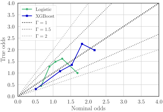
This figure shows a reliability diagram comparing observed odds ratios to predicted odds ratios from logistic and XGBoost models. The models aim to estimate the probability of an individual being sampled from the target population given their covariates, p(S=0|X). The reliability diagram visually assesses the calibration of these models. A perfectly calibrated model would show points along the diagonal line. Deviations from the diagonal indicate miscalibration, with points above the line suggesting overestimation and points below underestimation of the probability. The plot helps assess the credibility of the models used to handle sampling bias.

This figure shows how to benchmark credible values for the parameter Γ, which represents the degree of miscalibration allowed in the model of the sampling pattern. Panel (a) uses a real-world dataset to show how omitting different variables impacts the selection odds, providing a range for credible Γ values. Panel (b) then shows the impact of those Γ values on the inference of blood mercury levels in a target population under different seafood consumption policies.
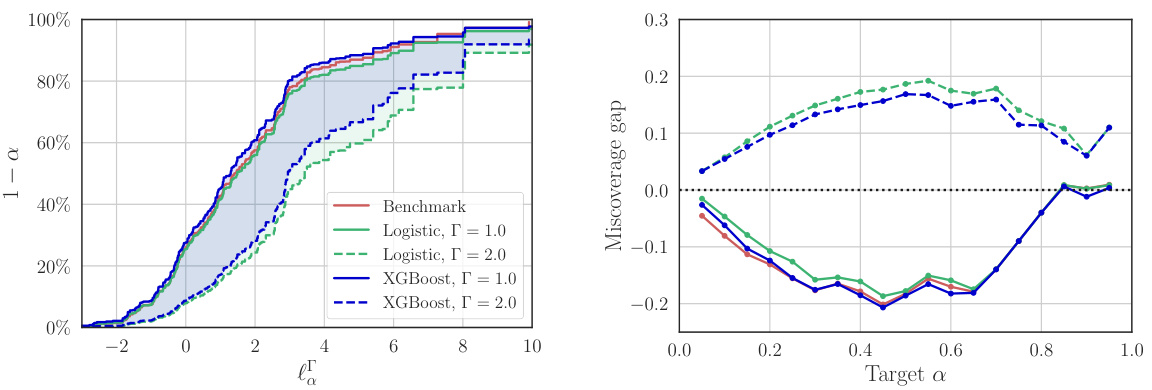
This figure shows the results of an experiment to evaluate the out-of-sample losses of a policy π using different methods. Subfigure (a) shows limit curves that bound the loss L with a given probability. The RCT-based curve only uses trial data, while other curves incorporate additional data from the target population and a sampling model to improve generalization. Subfigure (b) shows the gap between the actual and nominal probabilities of exceeding the loss limit, indicating the validity of the inferences.

This figure shows the results of an experiment evaluating the out-of-sample losses of a policy. Subfigure (a) displays limit curves showing the upper bound of the loss with a certain probability. The curves are generated using different methods, some incorporating additional data from the target population. Subfigure (b) shows the difference between the expected and actual probabilities of exceeding the loss limit, demonstrating the validity and conservatism of the approach.
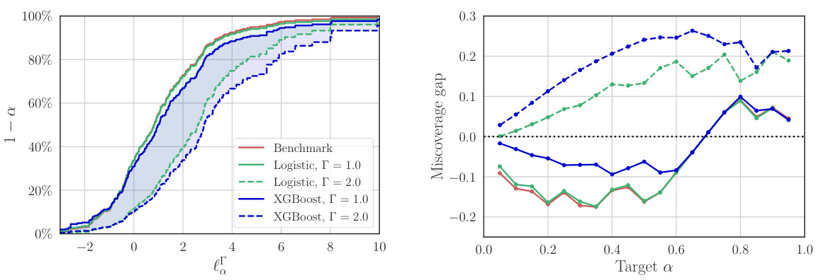
This figure shows the results of an experiment to infer the out-of-sample losses of a policy. The left subplot (a) displays limit curves showing the upper bound of the loss with a specified probability (1-α). The curves based on RCT data alone are compared to curves that also incorporate a sampling model trained on additional data from the target population. The right subplot (b) shows the difference between the actual and nominal probabilities of exceeding the loss limit, illustrating the validity of the inferences.
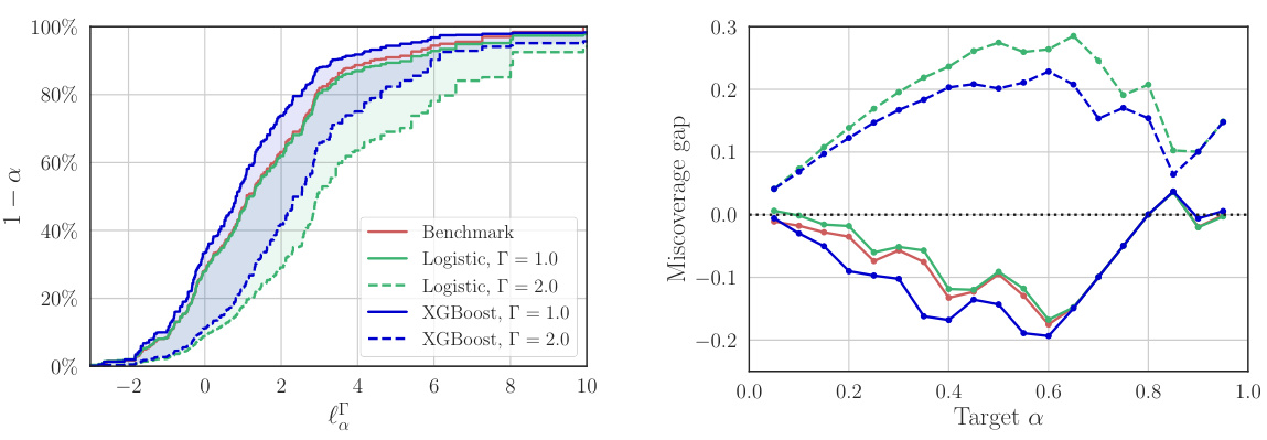
This figure shows how to infer out-of-sample losses using a policy. The left graph (a) shows that the loss L is bounded by an upper limit, and the right graph (b) shows that the inference is valid but conservative when there is a positive gap between the actual probability of exceeding the limit and the nominal probability of miscoverage.
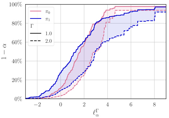
This figure shows how to infer out-of-sample losses for a given policy π. The left panel (a) shows how the loss L is bounded by an upper limit with probability 1-α. It compares limit curves obtained using only Randomized Controlled Trial (RCT) data versus additional covariate data from the target population, showing the benefits of including the extra data for making valid inferences. The right panel (b) displays the gap between the actual and nominal probabilities of exceeding the limit, illustrating the method’s accuracy and conservativeness.

This figure shows the results of an experiment to estimate the out-of-sample losses of a policy using both trial data and additional covariate data from the target population. Panel (a) displays limit curves showing an upper bound on the loss with a given probability. The curves based on trial data alone are valid only for the trial population, while curves using the sampling model trained on additional data are valid for the target population. Panel (b) shows the miscoverage gap, which indicates the validity of the inferences and shows the performance of the method for various degrees of model miscalibration.
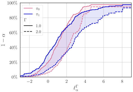
This figure shows the results of inferring out-of-sample losses of a policy using two methods. The first method uses only randomized controlled trial (RCT) data, while the second method incorporates additional covariate data from the target population and a sampling model. Subfigure (a) displays limit curves showing the upper bound of the loss with a specified probability. Subfigure (b) shows the difference between the actual and nominal probabilities of exceeding the loss limit, indicating the validity and conservatism of the inferences.
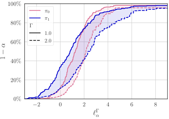
This figure shows the results of an experiment to evaluate the out-of-sample losses of a policy (π). Subfigure (a) compares different methods for bounding the loss, showing how the inclusion of additional data from the target population improves the accuracy and validity of the bounds. Subfigure (b) analyzes the accuracy of the loss bounds by plotting the miscoverage gap against the target miscoverage probability (α). A positive gap indicates the inference is valid but conservative, while a negative gap indicates it is invalid.

This figure compares the true selection odds (the ratio of probabilities of an individual being from the target population given covariates X to that of being from the trial population) against the selection odds predicted by two models: a logistic model and an XGBoost model. The plots show the odds ratio on the y-axis and x0 (one of the covariates) on the x-axis. The color gradients represent varying values of x1 (the other covariate). The dots represent a random subset of data points from the trial population. This visual comparison helps to assess the accuracy of the two different models in capturing the true relationship between the covariates and selection probability.
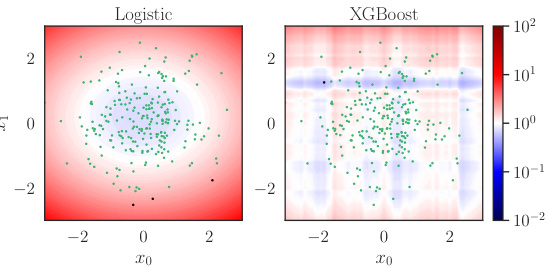
This figure compares the true selection odds, p(S=0|X)/p(S=1|X), which represent the ratio of probabilities of an individual belonging to the target population versus the trial population given their covariates X, against the estimated odds from two different models: a logistic regression model and a gradient boosted tree model (XGBoost). The plots show heatmaps representing the odds from each model and the true odds, with dots indicating a random subset of data points from the trial sample. This visualization helps to assess the accuracy and calibration of the probability models used for estimating the selection odds, which is crucial for accurate policy evaluation.

This figure compares the true selection odds (p(S=0|X)/p(S=1|X)) with the selection odds predicted by two different models (logistic and XGBoost) using data from the trial population. The heatmaps represent the predicted odds and the dots show a random sample from the trial data. This visualization helps to understand the quality of the two models in predicting the selection mechanism, crucial for the method proposed in the paper.
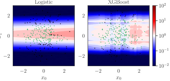
This figure compares the true selection odds, p(S=0|X)/p(S=1|X), to the selection odds predicted by two different models: a logistic model and an XGBoost model. The true selection odds are unknown, but the figure displays them to benchmark the accuracy of the models. Each model gives a prediction of the probability that a data point comes from the target population versus the trial population, given the covariates X. This figure illustrates how well the models can predict the selection odds. For each model, a heatmap shows the odds predicted by the model for different values of covariates. These heatmaps are overlaid with points representing a random subsample from the trial data, colored by whether they originate from the trial population (green) or the target population (black). This visualization helps to assess how well the model captures the actual selection process and to benchmark the choice of models and hyperparameters for the next steps of the proposed method.
More on tables

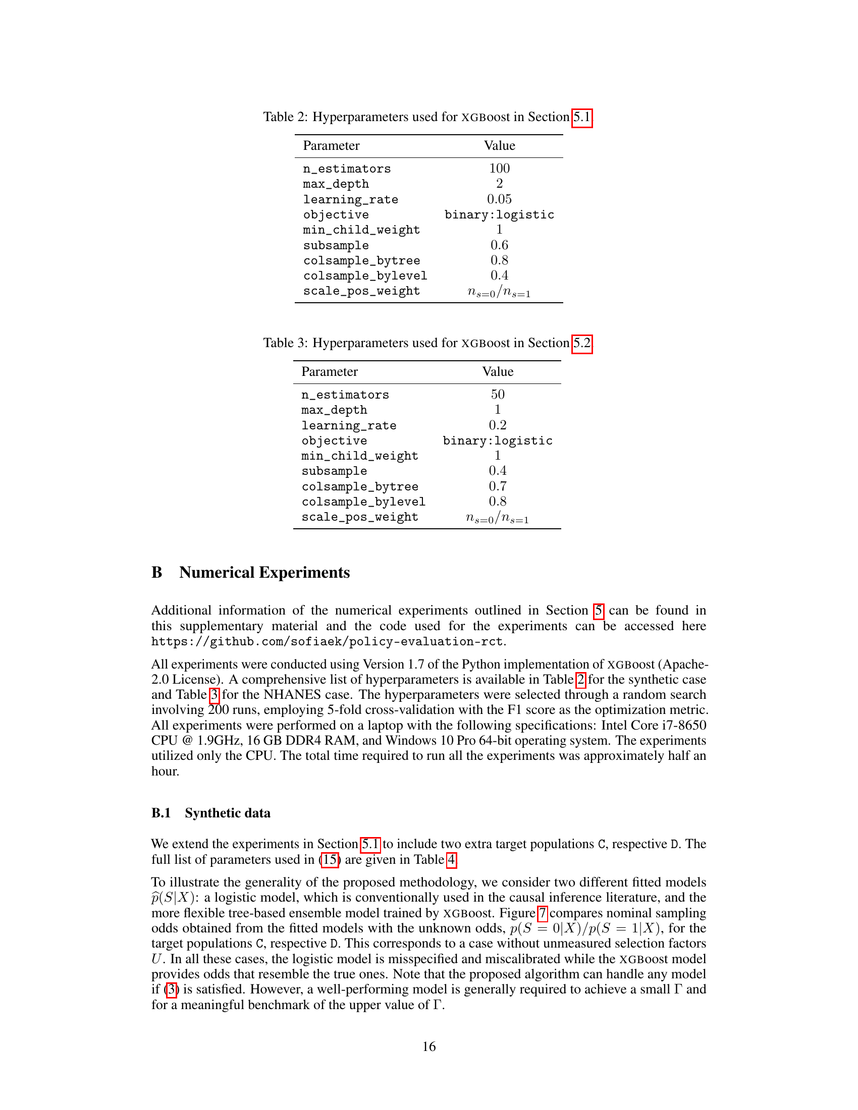
This table lists the hyperparameters used for training the XGBoost model in Section 5.1 of the paper. The XGBoost model is used for policy evaluation, specifically for modeling the sampling pattern of individuals in the trial and target populations. The hyperparameters control various aspects of the model’s training process, such as the number of trees, tree depth, learning rate, and regularization parameters. These settings are crucial for achieving a well-calibrated model that accurately reflects the relationship between covariates and the sampling probability.
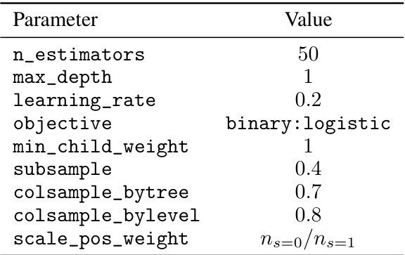
This table lists the hyperparameters used for training the XGBoost model in Section 5.2 of the paper, which focuses on real-world data experiments involving seafood consumption and blood mercury levels. The hyperparameters control various aspects of the model’s training process, such as the number of trees, tree depth, learning rate, objective function, minimum child weight, subsampling ratio, and column subsampling ratio. The
scale_pos_weightparameter addresses class imbalance in the dataset.

This table presents the means (μ) and variances (σ²) of the covariate distributions used in the synthetic data experiments. The distributions are for two-dimensional covariates X and an unmeasured selection factor U, conditioned on the sampling indicator S (0 for target, 1 for trial). Four different target populations (A, B, C, D) are shown, along with the trial population. The values allow for a controlled level of covariate shift between the trial and target populations. These distributions are used in Equation 15 of the paper.
Full paper#

