↗ OpenReview ↗ NeurIPS Homepage ↗ Chat
TL;DR#
AI systems often struggle with generalizing predictions to new, unseen domains. Existing methods often lack performance guarantees. This is particularly concerning for safety-critical AI applications. The unpredictable nature of new data distributions makes reliable performance assessment difficult. This paper tackles the challenge of providing such performance guarantees.
The researchers propose a new method based on the theory of partial identification and causal transportability. They leverage causal diagrams to model data generation processes and develop a general estimation technique to compute upper bounds for prediction errors. Their approach is both rigorous and practical, introducing a gradient-based optimization scheme for scalability and demonstrating effectiveness through experiments with both simulated and real-world datasets. This leads to improved performance guarantees, particularly valuable for high-stakes AI applications.
Key Takeaways#
Why does it matter?#
This paper is crucial for AI safety and reliability, offering the first general technique to bound prediction errors in unseen domains. It bridges causal inference and machine learning, opening avenues for robust AI development and addressing a fundamental challenge in generalization.
Visual Insights#

This figure illustrates the challenge of evaluating a model’s performance in a new, unseen domain (target domain). Two source domains (M¹, M²) with data distributions P¹ and P² are used to train a model h. The causal mechanisms governing the variables C, W, Y, and Z (where Y is the outcome variable and C and W are covariates) differ across domains. The goal is to infer the target risk Rp*(h) (the expected performance on the target domain M*) based only on data from the source domains and assumptions encoded in a causal diagram (not explicitly shown in this figure but described in the paper). The core issue is the non-transportability of the target domain risk, meaning we cannot directly estimate Rp*(h) from source domain data alone.
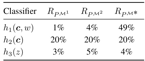
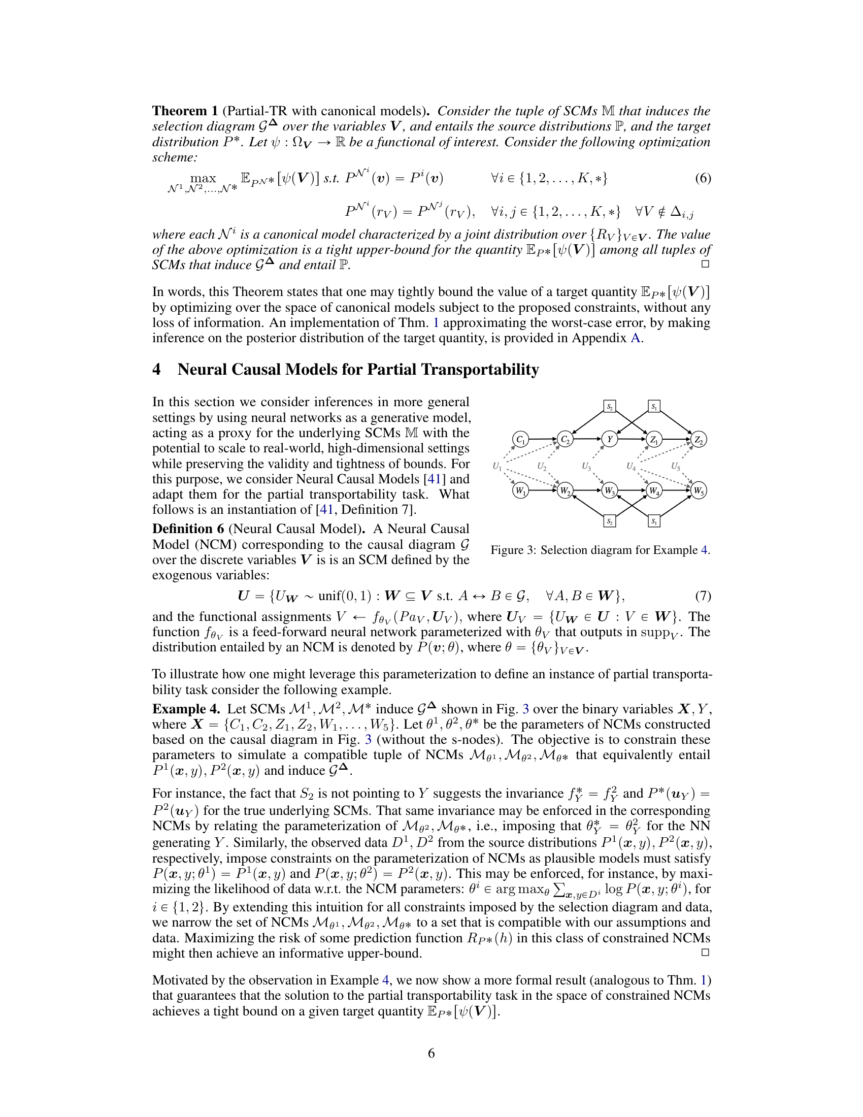
This table presents the performance (error rate) of three different classifiers (h1(c,w), h2(c), and h3(z)) across three different domains (M1, M2, M*). The classifiers use different sets of variables (c, w, z) as input, highlighting the impact of feature selection on generalization performance. Noteworthy is the difference in performance of the classifiers in the target domain (M*) compared to the source domains (M1, M2).
In-depth insights#
Partial Transportability#
Partial transportability, in the context of domain generalization, tackles the challenge of making inferences about a target domain using data from related source domains when a complete transfer is impossible. This approach acknowledges inherent uncertainties about the target domain’s data distribution. It leverages causal diagrams and assumptions about the data generating mechanisms to establish bounds on target quantities, such as generalization error, rather than aiming for exact predictions. By quantifying the uncertainty associated with the transfer, partial transportability offers a more robust and reliable approach to domain generalization, particularly relevant when complete data invariance across domains is unrealistic. Key to this method is the integration of causal knowledge to guide the generalization process and to constrain the range of possible outcomes in the target domain, hence providing more informative bounds than purely statistical approaches.
Causal Risk Bounds#
The concept of “Causal Risk Bounds” in a research paper would likely explore how causal inference can be used to provide tighter and more informative bounds on the risk of a machine learning model. Traditional risk analysis often relies on statistical correlations, which can be misleading due to confounding factors and lack of causal understanding. Causal risk bounds aim to address this limitation by explicitly modeling causal relationships within the data, using causal diagrams and assumptions about the data-generating process. This allows for a more robust assessment of model performance, particularly in out-of-distribution settings or when dealing with interventions. By considering causal pathways and mechanisms, these bounds could provide a more accurate representation of the actual risk, moving beyond merely correlational measures. The resulting insights would be useful for enhancing model robustness and reliability. This approach may particularly focus on identifying the worst-case scenarios based on plausible causal models and their associated uncertainties which is very useful for safety-critical applications.
Neural Causal Models#
The application of Neural Causal Models (NCMs) in the paper presents a novel approach to tackling the challenge of partial transportability in domain generalization. NCMs offer a flexible and scalable framework capable of handling high-dimensional data and complex causal relationships, surpassing the limitations of traditional methods. By encoding qualitative assumptions about causal mechanisms into the model architecture, NCMs allow for the integration of domain-specific knowledge, leading to more robust and accurate inferences. The use of gradient-based optimization techniques enables scalable inference, a critical advantage in practical settings. However, the reliance on NCMs also introduces complexities, including the need for careful parameterization and the potential for overfitting. The paper successfully demonstrates the effectiveness of NCMs through empirical results, highlighting their potential for advancing the field of domain generalization. Further research is needed to fully explore the potential and limitations of this approach in various application domains, especially considering the challenges associated with model interpretability and generalization to unseen data.
CRO Optimization#
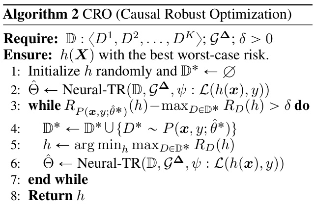
The heading ‘CRO Optimization’ likely refers to Causal Robust Optimization, a novel algorithmic approach proposed in the research paper for tackling domain generalization challenges. This method leverages the theoretical framework of partial transportability, which allows for bounding the performance of a prediction model even under significant uncertainty about the target domain. CRO iteratively refines a classifier by using Neural-TR, an algorithm that identifies the worst-case target domain given the source data and causal assumptions. By iteratively training on the worst-case scenario, CRO aims to improve the classifier’s robustness. This is a significant advancement, as it moves beyond simply minimizing average risk to guaranteeing performance bounds in unseen environments. The efficacy of this approach is evaluated on both synthetic and real-world datasets, showcasing its capacity to improve generalizability compared to existing techniques. A key strength lies in its ability to effectively utilize causal structure to construct robust models in challenging, non-transportable settings.
Future Directions#
Future research could explore extensions to handle more complex causal structures and unobserved confounders, improving the accuracy and robustness of partial transportability methods. Investigating the impact of different loss functions and model architectures on the bounds and scalability of these methods is also crucial. A deeper understanding of the relationships between the various types of uncertainty (aleatoric, epistemic) and the performance of these techniques warrants further investigation. Developing more efficient algorithms for optimizing the worst-case risk while considering computational complexity in high-dimensional settings would broaden the practicality of this work. Additionally, empirical evaluations on a wider range of real-world datasets, exploring different application domains, is necessary to demonstrate the effectiveness and generalizability of this approach in practice. Finally, exploring connections with other domain generalization techniques and hybrid approaches could offer synergistic advantages and a more comprehensive approach to tackling this challenge.
More visual insights#
More on figures

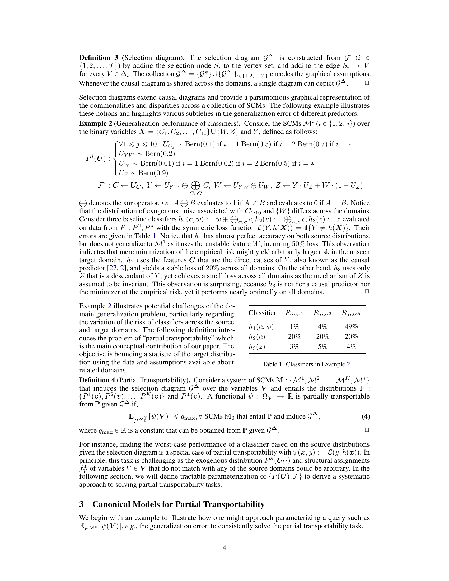
This figure illustrates the selection diagram and canonical parameterization for Example 3 (The bow model). The selection diagram (a) shows the relationships between variables X and Y in multiple SCMs, including source domains and target domains, and how discrepancies (indicated by the selection nodes S1 and S2) affect transportability. The canonical parameterization (b) represents a simplified SCM model with correlated discrete latent variables Rx and Ry used for consistently solving the partial transportability task by reducing the dimensionality and complexity of the problem.

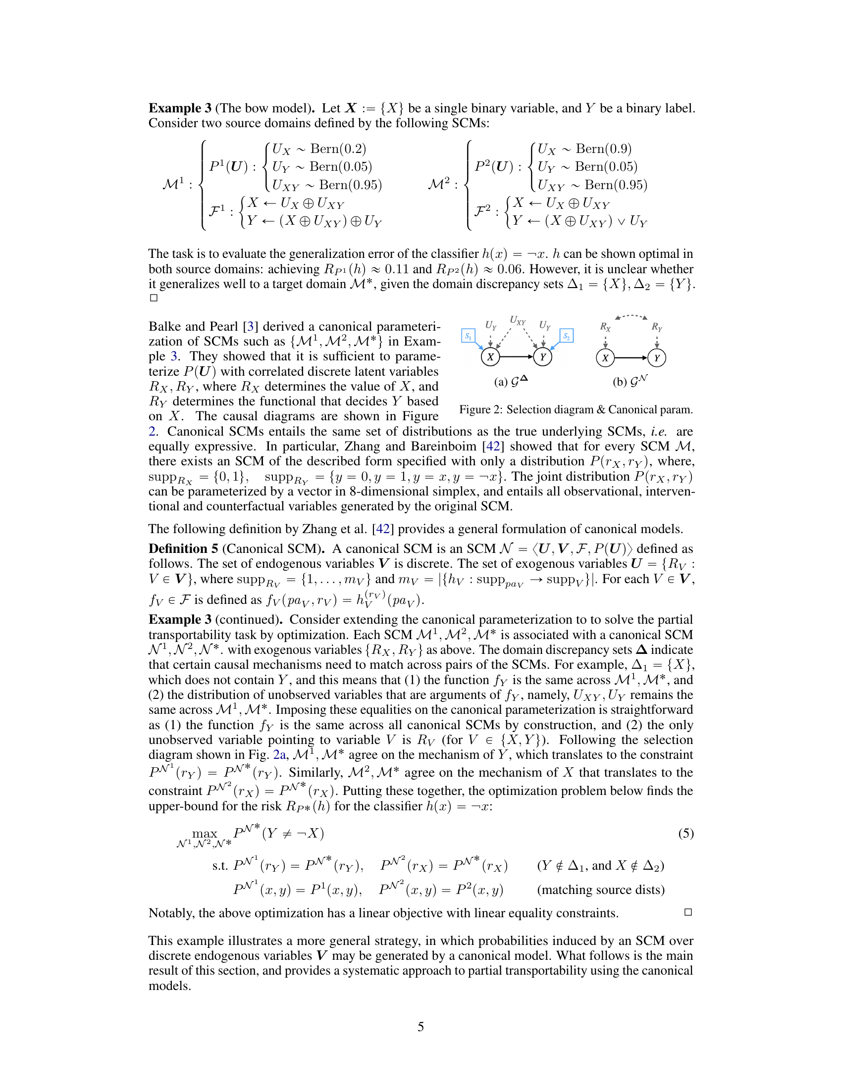
This selection diagram shows the causal relationships between variables in Example 4 of the paper. The diagram illustrates how the variables C, W, Y, Z are causally related, as well as how the selection nodes S1 and S2 impact the observation of these variables across different domains. The dashed lines represent potential discrepancies in the causal mechanisms between source and target domains, indicated by the selection node. This highlights the complexities in domain generalization, where a model trained on source domains may not generalize well to the target domain due to differences in these underlying causal mechanisms.

This figure shows the results of worst-case risk evaluation experiments using two algorithms: Neural-TR and CRO. Subfigures (a), (b), and (c) display the worst-case risk (y-axis) over training iterations (x-axis) for three different scenarios (Example 2, Example 3, and CMNIST dataset). The plots show how the worst-case risk converges as the algorithms train. Subfigures (d) and (e) show the worst-case risk obtained after training with CRO for Example 2 and Example 3, respectively. These plots illustrate the effectiveness of the algorithms in finding tight upper bounds on the generalization error.

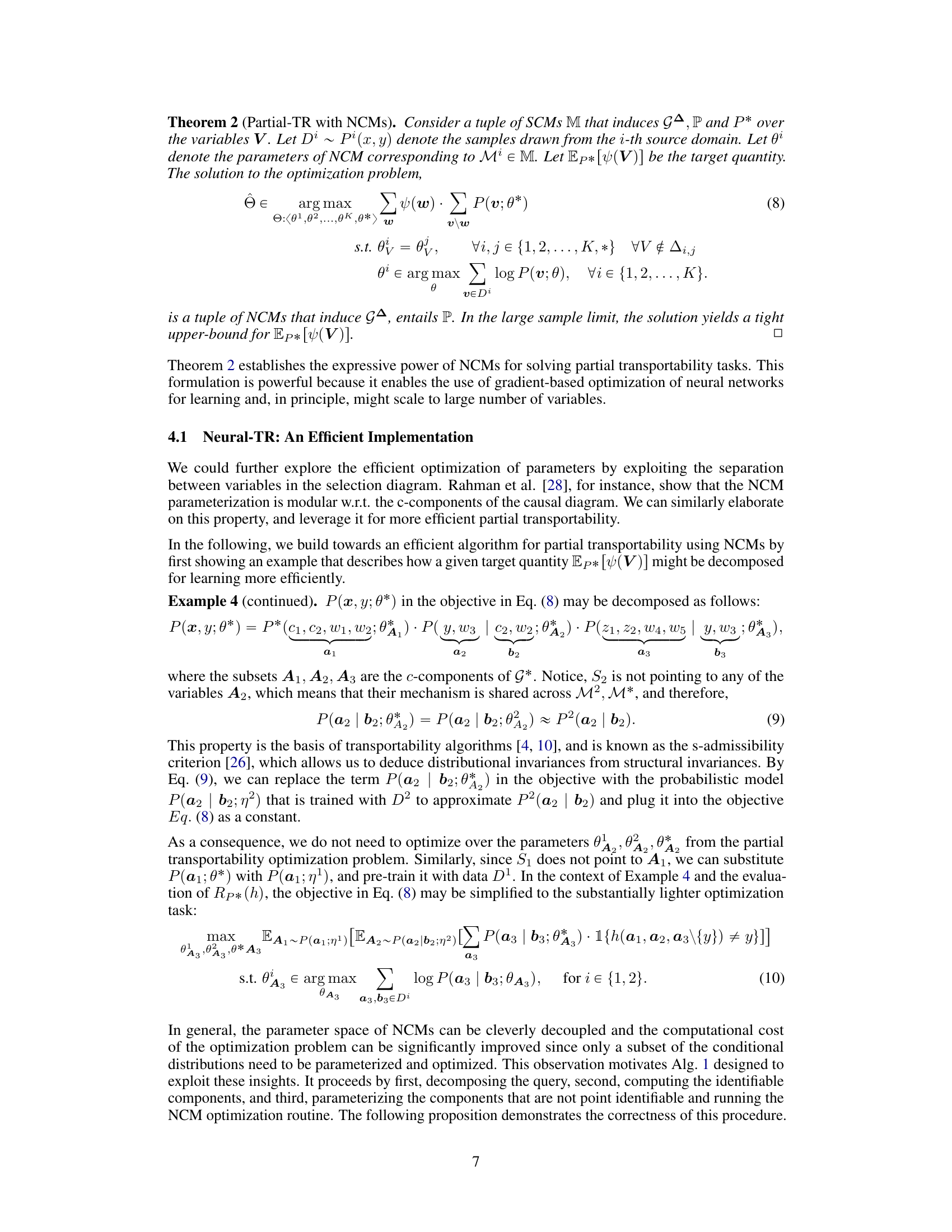
This figure shows the causal graph used in the Colored MNIST experiment. The variables represent: W (grayscale MNIST image), C (color, red or green), Y (binary label, whether the digit is 5 or greater), and Z (colored image). The dashed arrows from W indicate that the mechanism for W might differ across domains. The nodes S1 and S2 represent selection nodes indicating that there might be discrepancies in the mechanisms of C across domains.

The figure shows the results of worst-case risk evaluation using Neural-TR and CRO algorithms for Examples 2 and 3, and CMNIST dataset. The plots (a-c) illustrate how the worst-case risk converges over training iterations for different classifiers (h1, h2, h3 in Example 2; h1, h2, h3, h4 in Example 3; hERM, hIRM, hDRO in CMNIST). The plots (d,e) display the worst-case risk obtained by CRO, comparing it with the performance of other classifiers. The results demonstrate the effectiveness of Neural-TR in assessing worst-case risk and the ability of CRO to find optimal classifiers under worst-case scenarios.

The figure shows the results of worst-case risk evaluation for different classifiers using two different methods. (a-c) show the worst-case risk evaluation using Neural-TR (Algorithm 1), plotting the worst-case risk against the number of training iterations for three different examples. (d,e) show the worst-case risk evaluation using CRO (Algorithm 2) for two of the examples. Each subfigure shows how the worst-case risk converges over training iterations (or epochs).

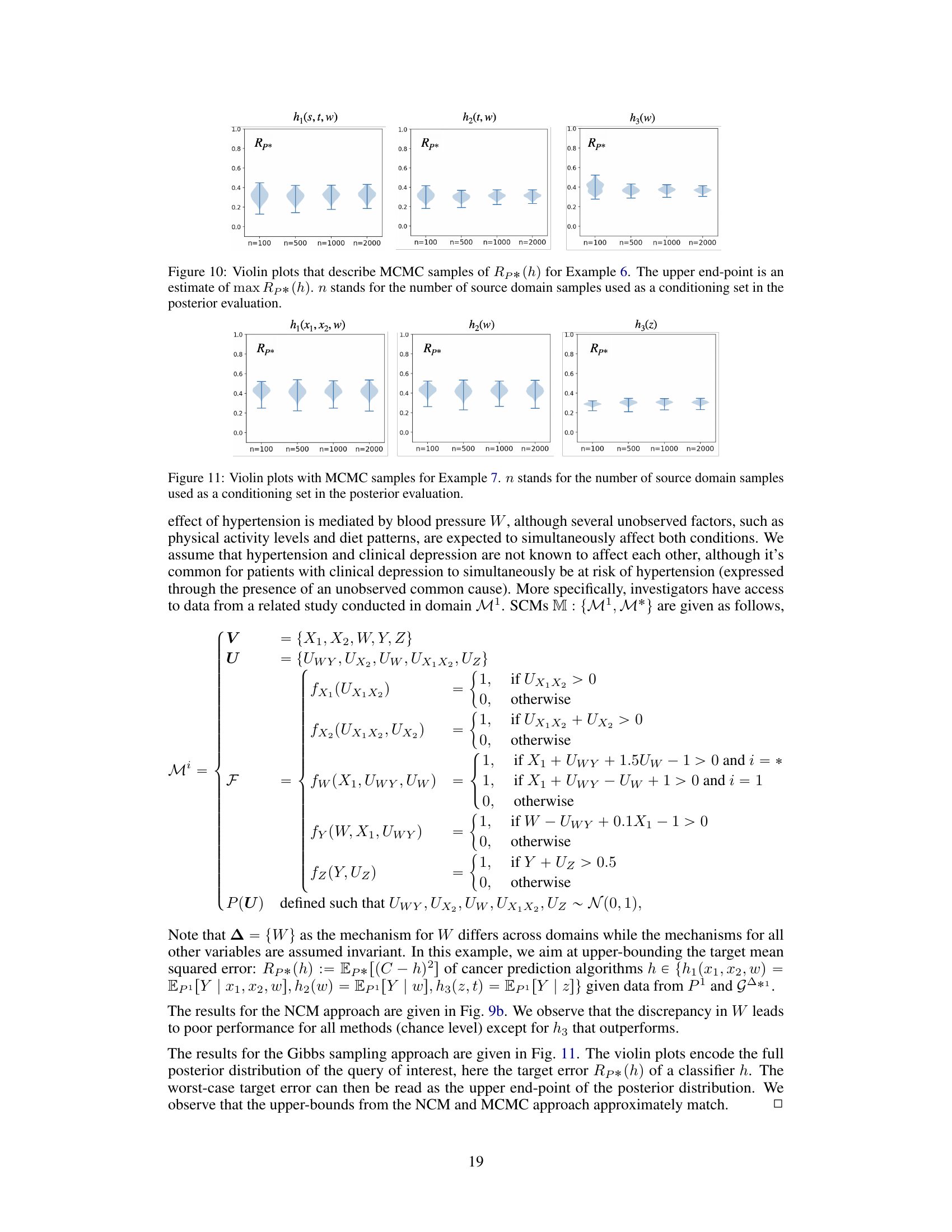
This figure presents the results of applying Neural Causal Models (NCMs) to two examples (Example 6 and 7) from the paper. Each example involves a causal inference task where the goal is to estimate the risk of different classifiers in a target domain. The figure shows the worst-case risk evaluated by the Neural-TR algorithm across training epochs. The plots compare the performance of multiple classifiers which differ in the variables they use to make predictions. This helps to understand how well the classifiers generalize from source data to a new, unseen domain (M*). The left plot shows results for Example 6 (lung cancer) while the right shows results for Example 7 (Alzheimer’s disease).

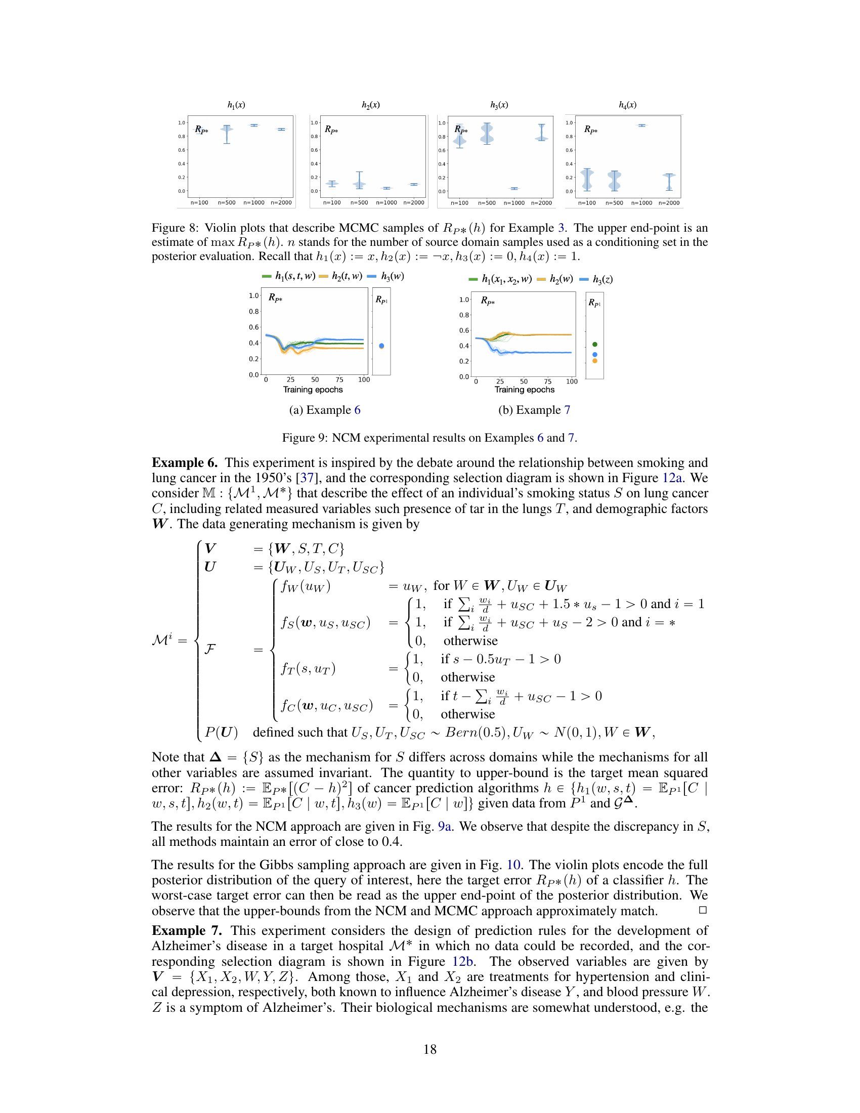
Violin plots showing the results of a Markov Chain Monte Carlo (MCMC) sampling method used to estimate the worst-case risk (Rp*) for different classifiers (h1, h2, h3) in Example 6 of the paper. The x-axis represents the number of samples (n) from source domains used as conditioning data in the posterior estimation, and the y-axis represents the worst-case risk (Rp*). Each violin plot shows the distribution of the estimated worst-case risks, and the upper end-point of each violin represents an estimate of the maximum worst-case risk.

The figure shows the worst-case risk evaluation results obtained by applying Neural-TR and CRO algorithms on different examples, including simulated examples and the colored MNIST dataset. Subfigures (a), (b), and (c) illustrate the convergence of worst-case risk evaluation using Neural-TR as a function of the number of training iterations for three different examples (Examples 2, 3, and CMNIST). Subfigures (d) and (e) show the worst-case risk evaluations obtained with the CRO algorithm for Examples 2 and 3, respectively. These results demonstrate the effectiveness of the proposed algorithms in bounding the worst-case generalization error in different scenarios.

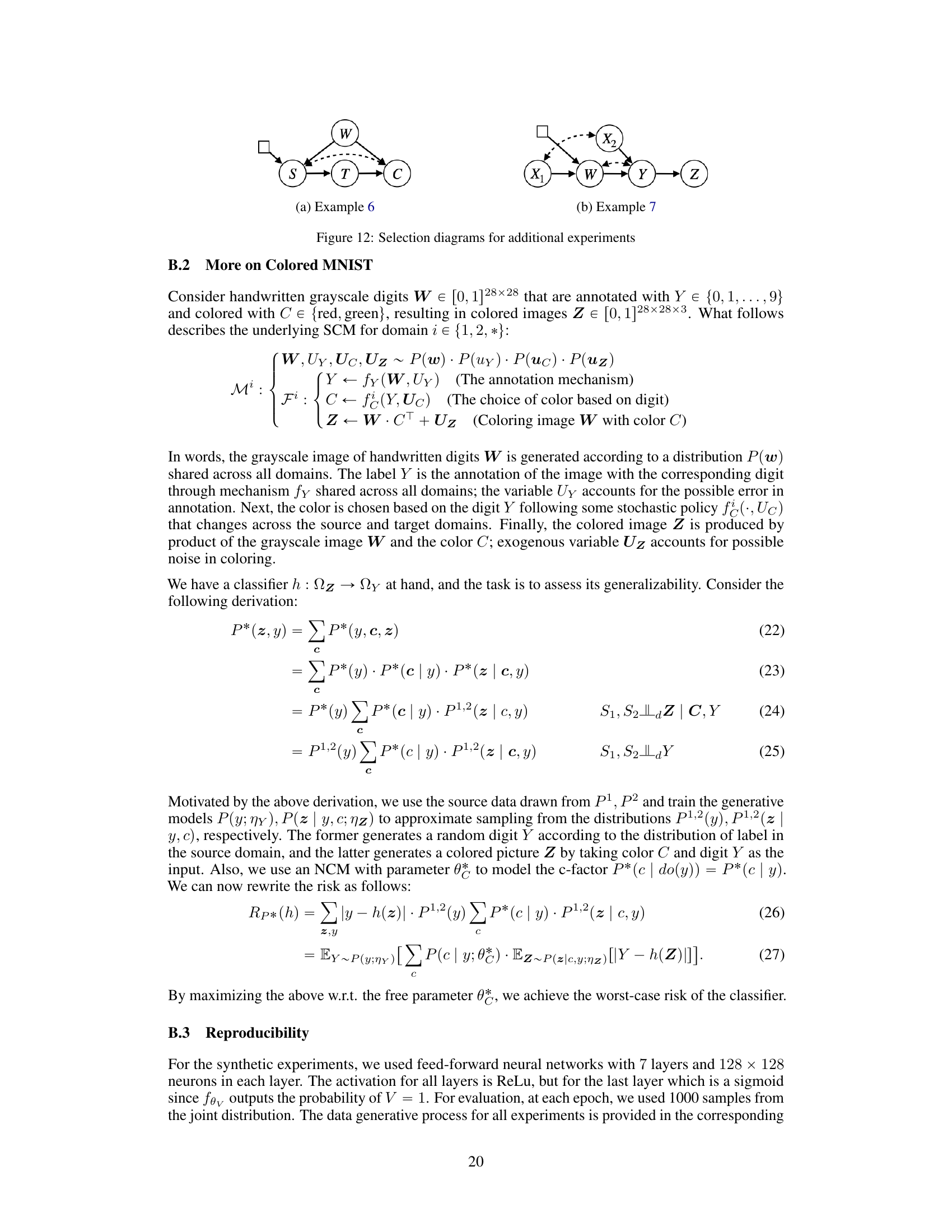
This figure presents two selection diagrams used in additional experiments presented in Appendix B. The diagrams graphically represent the relationships between variables and assumptions about which variables’ mechanisms are invariant across domains. (a) shows the diagram for Example 6, a study of smoking and lung cancer. (b) shows the diagram for Example 7, which explores the prediction of Alzheimer’s disease. These diagrams are crucial for applying the Partial Transportability framework, highlighting the causal relationships and discrepancies between the source and target domains.

This selection diagram shows the causal relationships between variables in Example 4 of the paper. The variables are denoted by circles, and the arrows indicate the direction of causality. The dashed lines represent the domain discrepancies, meaning that the mechanisms governing the relationships between the variables are not the same in all domains. This is important for the task of partial transportability because the goal is to compute bounds on statistical queries in the target domain given only data from source domains and assumptions about the causal relationships. By encoding these assumptions in the selection diagram, the researchers can more effectively leverage source data to make inferences about the target domain.
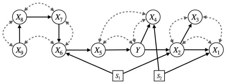
The figure shows two selection diagrams, (a) and (b), which represent the graphical assumptions for two additional experiments described in Appendix B. Selection diagrams extend causal diagrams by adding selection nodes to represent domain discrepancies. In diagram (a), the discrepancy set for Example 6 is {S}, meaning the mechanism for variable S (smoking status) may differ across domains, while the mechanisms for other variables (tar in the lungs, lung cancer, etc.) are assumed invariant. Diagram (b) shows the selection diagram for Example 7, where the discrepancy set is {W} (blood pressure). This indicates that the mechanism for blood pressure may vary across domains, while other variables related to Alzheimer’s disease (treatments for hypertension and clinical depression, a symptom of Alzheimer’s) are assumed invariant.

This figure illustrates the iterative process of Causal Robust Optimization (CRO). It shows how Neural-TR finds increasingly difficult target distributions, while DRO adapts the classifier to minimize the maximum risk across seen distributions. The process continues until an equilibrium is reached, where the worst-case risk is minimized.
More on tables
The table shows the performance of three different classifiers (h1, h2, h3) across three different domains (M1, M2, M*). The classifiers use different sets of features (c, w, z), and their performance is measured by the risk (Rp) which represents the prediction error. Example 2 in the paper highlights that simply minimizing empirical risk on source domains does not guarantee good generalization to the target domain. The table illustrates how different choices of features affect the generalization performance.

This table presents the performance of three different classifiers (h1, h2, h3) across three domains (M1, M2, M*). The classifiers differ in the variables they use as input features. The table shows the risk (error rate) of each classifier in each domain, illustrating how performance can vary significantly across domains and highlighting the challenges of generalizing from source domains to unseen target domains.
Full paper#


