↗ OpenReview ↗ NeurIPS Homepage ↗ Chat
TL;DR#
Constrained Reinforcement Learning (CRL) tackles sequential decision-making problems with constraints, often using policy-based methods. However, existing policy-gradient methods often lack global convergence guarantees, especially when dealing with continuous control and multiple constraints, or risk measures in safety-critical scenarios. This limits their real-world applicability.
This paper introduces C-PG, a novel primal-dual algorithm that offers global last-iterate convergence guarantees under weak assumptions, addressing limitations of existing approaches. It further presents C-PGAE and C-PGPE, action- and parameter-based versions of C-PG, respectively, and extends them to handle risk-measure constraints. Numerical validation confirms their improved performance on various constrained control problems.
Key Takeaways#
Why does it matter?#
This paper is important because it provides globally convergent algorithms for constrained reinforcement learning (CRL), a crucial area in AI. It offers dimension-free convergence guarantees, improves existing CRL methods and extends their applicability to various risk measures, opening new avenues for safer and more robust AI applications.
Visual Insights#

This figure is a plot showing the exponents of epsilon inverse in the sample complexity results of the C-PG algorithm. It illustrates how the sample complexity scales differently depending on whether the gradients are exact or estimated and the value of psi (ψ). The plot helps visualize the trade-off between computational cost and convergence rate.

This table summarizes the sample complexity results of the C-PG algorithm under different conditions. It shows how the sample complexity scales with epsilon (ε) and the regularization parameter (ω) for both exact and estimated gradients, and for different values of ψ (a parameter related to the gradient domination condition). The table distinguishes between keeping ω fixed or setting it to be a function of ε. The results indicate that the algorithm’s complexity varies based on the presence of gradient noise and the strength of the gradient domination.
In-depth insights#
CRL via Primal-Dual#
Constrained Reinforcement Learning (CRL) presents a unique challenge in reinforcement learning by requiring agents to optimize rewards while adhering to constraints. Primal-dual methods offer an elegant approach to address this challenge by converting the constrained optimization problem into an unconstrained one using Lagrange multipliers. The primal problem focuses on optimizing the reward function, while the dual problem manages the constraints via the Lagrange multipliers. Iterative updates to both primal and dual variables allow the algorithm to converge to a solution that satisfies both the reward objective and the constraints. The effectiveness of this approach rests on carefully balancing the exploration-exploitation tradeoff. Gradient-based methods are often employed within the primal-dual framework; they update parameters using gradients to efficiently search the solution space. The last-iterate convergence guarantees offered by the method demonstrate the algorithm’s robustness and stability, ensuring that the final solution indeed satisfies the constraints. The use of risk measures in CRL further enhances its applicability to safety-critical scenarios. Risk-averse approaches allow the algorithm to account for uncertainty and achieve safety guarantees. The primal-dual framework is highly adaptable and can incorporate various algorithms, risk measures, and constraint types. Thus, it offers a powerful and flexible solution to address the complexities of CRL.
C-PG Algorithm#
The C-PG algorithm, presented within the context of constrained reinforcement learning (CRL), is a novel primal-dual method designed for optimizing a regularized Lagrangian function. Its key innovation lies in achieving global last-iterate convergence guarantees under weak gradient domination assumptions, a significant improvement over existing methods which often only guarantee convergence to a stationary point or rely on stronger assumptions. The algorithm’s strength comes from its exploration-agnostic nature, making it compatible with both action-based and parameter-based policy gradient approaches. This adaptability extends to various constraint formulations, including those defined in terms of risk measures, enhancing its applicability to safety-critical domains. Dimension-free convergence rates further solidify its potential for solving large-scale CRL problems. In essence, C-PG offers a robust and theoretically well-founded approach to policy optimization in CRL, pushing the boundaries of current state-of-the-art techniques.
Risk-Constrained RL#
Risk-constrained reinforcement learning (RL) addresses the limitations of standard RL in scenarios demanding safety and reliability. Traditional RL methods focus solely on maximizing cumulative reward, often neglecting the potential for catastrophic failures. Risk-constrained RL incorporates risk measures, allowing agents to balance reward maximization with the mitigation of undesirable outcomes. This is crucial in real-world applications like robotics and autonomous systems where safety is paramount. Several techniques are employed to achieve this balance, including chance constraints, conditional value at risk (CVaR), and mean-variance optimization. The choice of risk measure depends heavily on the specific application and its risk tolerance. The introduction of constraints necessitates sophisticated algorithms that effectively manage the trade-off between reward and risk. Primal-dual methods and Lagrangian optimization are commonly used to achieve this. While the field is rapidly advancing, challenges remain, including the computational cost of managing constraints and ensuring algorithm convergence in complex environments. Future research should focus on developing more efficient algorithms and addressing scalability issues to allow wider adoption of risk-constrained RL in high-stakes applications.
Convergence Rates#
Analyzing convergence rates in optimization algorithms is crucial for evaluating their efficiency. Faster convergence translates to fewer iterations and potentially less computational cost. The paper likely investigates how different algorithmic choices (e.g., primal-dual methods, different policy gradient exploration approaches) affect the convergence speed. It is important to distinguish between global and local convergence: global convergence assures that the algorithm approaches the optimal solution from any starting point, whereas local convergence only guarantees this from a limited neighborhood of the optimum. A key aspect will be determining if the rates are dimension-free—independent of the state and action space dimensions—essential for scalability to real-world applications. The analysis may involve theoretical bounds, demonstrating the algorithm’s convergence rate under certain assumptions. Last-iterate convergence, where the final iterate converges to the solution, is a particularly desirable property. The study will likely compare various convergence rates across different algorithms, providing a valuable benchmark for future research and potentially highlighting optimal algorithmic strategies for constrained reinforcement learning problems. Finally, the impact of regularization techniques on convergence rates should be analyzed, weighing the improved convergence against any potential bias introduced.
Future Work#
The paper’s conclusion, while not explicitly labeled ‘Future Work,’ strongly suggests avenues for continued research. Improving sample complexity is paramount, particularly achieving dimension-free rates without the two-time scale approach currently used. This would enhance scalability and applicability to high-dimensional problems. Another key direction is extending the algorithm’s scope beyond risk measures currently implemented, such as exploring different risk-averse formulations and their associated theoretical challenges. The authors also hint at the possibility of developing algorithms that match sample complexity lower bounds, a highly valuable goal for enhancing efficiency. Finally, the work could benefit from a more in-depth analysis of the algorithm’s performance in a broader range of environments, including those with more complex dynamics and constraints, to ensure its generalizability. All in all, the authors have laid a solid foundation ripe for substantial future contributions.
More visual insights#
More on figures

This figure presents the results of the experiments conducted in two different environments: the Discrete Grid World with Walls (DGWW) and the Linear Quadratic Regulator with costs (CostLQR). The plots show the average trajectory return and the average trajectory cost over the number of trajectories observed during learning. Two separate subfigures display results for DGWW and CostLQR, each with multiple lines representing different algorithms. The shaded regions show the 95% confidence intervals. The figure highlights the performance of C-PGAE and C-PGPE in comparison to other algorithms (NPG-PD, RPG-PD, NPG-PD2, RPG-PD2).

The figure shows the empirical distributions of costs over 100 trajectories of the learned (hyper)policies via C-PGPE and C-PGAE for the Swimmer-v4 environment. Each subplot represents a different risk measure (average cost, CVaR, MV, and chance) used as a constraint during training. The table shows average return for each algorithm and risk measure. The results illustrate how different risk measures affect the cost distribution and the overall performance of the learned policies.
This figure presents the results of applying the proposed C-PGAE algorithm and comparing it with other baselines (NPG-PD, RPG-PD, NPG-PD2, RPG-PD2) on two different environments: Discrete Grid World with Walls (DGWW) and Linear Quadratic Regulator with Costs (CostLQR). The plots show the average trajectory return and the average trajectory cost across 5 independent runs, with 95% confidence intervals displayed. The DGWW results demonstrate the learning performance of tabular softmax policies on a discrete environment. The CostLQR results demonstrate the performance of continuous gaussian policies on a continuous environment. In both cases, C-PGAE is shown to achieve comparable performance with fewer trajectories.
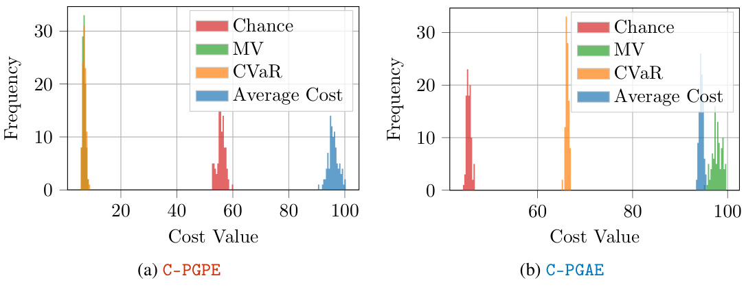
The figure shows the empirical distributions of costs over 100 trajectories of the learned (hyper)policies via C-PGPE and C-PGAE. This experiment considers the cost-based version of the Swimmer-v4 MuJoCo (Todorov et al., 2012) environment, with a single constraint over the actions (see Appendix H), for which we set b = 50. The experimental results show that C-PGPE learns a hyperpolicy paying less cost when using risk measures compared to average cost, with the smallest costs attained by CVaR. C-PGAE shows similar results, although the difference between CVaR or the Chance constraints and average cost constraints are not very significant. Notice that, the minimum amount of cost is obtained using MV constraints even if the learned policy exhibits poor performances (Table 3c). In all the other cases, both C-PGPE and C-PGAE learns (hyper)policies exhibiting similar performance scores.
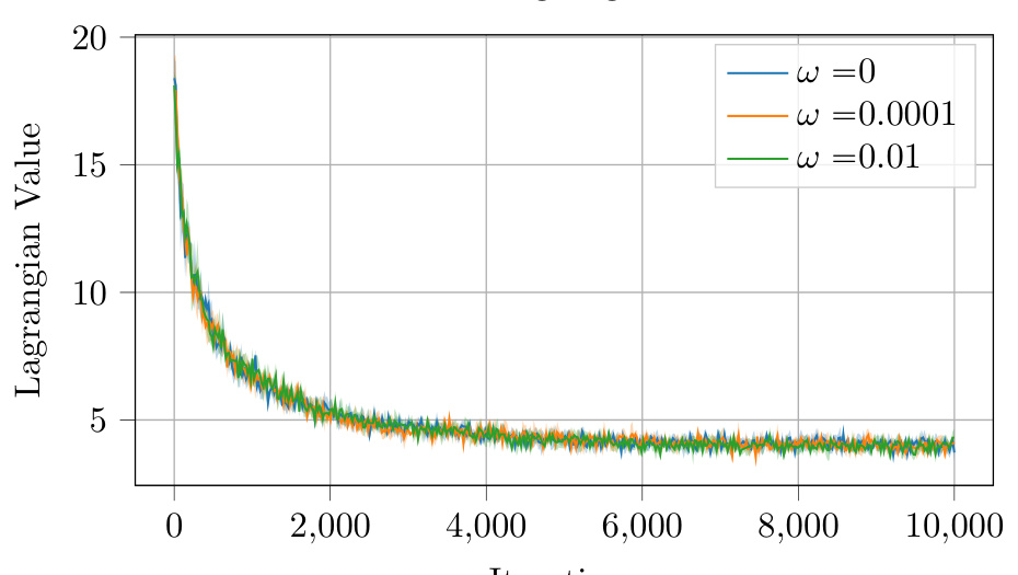
This figure displays the Lagrangian, performance (average trajectory return), and cost (average trajectory cost) curves for the C-PGPE algorithm over the CostLQR environment. The experiment compares the effect of different regularization values (ω ∈ {0, 10⁻⁴, 10⁻²}) on the algorithm’s convergence behavior and its ability to meet the specified cost constraint. Each curve represents the average over 5 runs, with 95% confidence intervals shown.

This figure shows the comparison results of the proposed algorithms (C-PGAE and C-PGPE) against state-of-the-art baselines in two different environments: a discrete grid world with walls (DGWW) and a continuous linear quadratic regulator with costs (CostLQR). The plots display the average trajectory return and the average trajectory cost over multiple independent runs, with 95% confidence intervals shown. The results illustrate the effectiveness of the proposed algorithms in achieving better performance in terms of both return and cost compared to baselines, particularly in the CostLQR environment. Note that the y-axis is in log scale for better visualization.
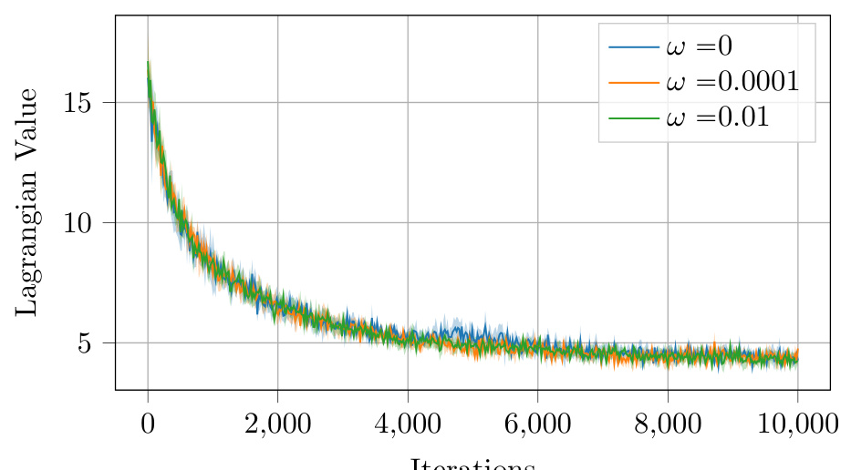
This figure shows the results of the regularization sensitivity study of the C-PGPE algorithm on the CostLQR environment. Three different regularization values (ω = 0, ω = 0.0001, ω = 0.01) were tested, and the plots show the average Lagrangian value, average trajectory return, and average trajectory cost over 10000 iterations. Each plot shows the mean and 95% confidence interval across 5 runs.

This figure presents the results of two experiments conducted to compare the performance of the proposed algorithms (C-PGAE and C-PGPE) against state-of-the-art baselines on two different environments. The first experiment uses a discrete grid world with walls (DGWW), and the second experiment employs a continuous linear quadratic regulator with costs (CostLQR). Both experiments involve a single constraint on the average trajectory cost. The plots show the average trajectory return and average trajectory cost over the course of training, demonstrating the effectiveness of the proposed algorithms in achieving the desired balance between maximizing return and satisfying constraints. Error bars represent 95% confidence intervals across 5 independent runs.
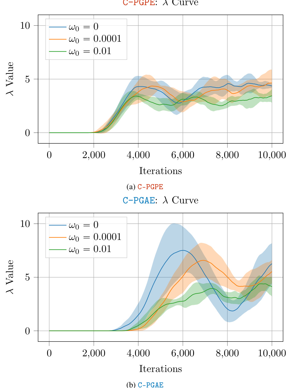
This figure shows the evolution of the Lagrangian multipliers λ during the learning process for both C-PGPE and C-PGAE algorithms, considering different regularization values (ω ∈ {0, 10⁻⁴, 10⁻²}). The plots illustrate how the Lagrangian multipliers, which represent the dual variables in the primal-dual optimization framework, adapt based on the level of regularization applied. The shaded areas show the 95% confidence interval for five independent runs of each experiment. The figure helps to visually understand the impact of regularization on the algorithm’s convergence behavior.
More on tables

This table shows how the unified risk measure formulation can be used to represent several risk measures by selecting appropriate functions fᵢ and gᵢ. It lists the risk measure, its parameter, whether an auxiliary parameter η is needed, the form of fᵢ(Cᵢ(τ), η), the form of gᵢ(η), whether an action-based GPOMDP-like estimator is available, and if so, whether it’s partial or not. The table clarifies how different risk preferences can be incorporated into the optimization problem by changing the parameters and functions in the unified formulation.
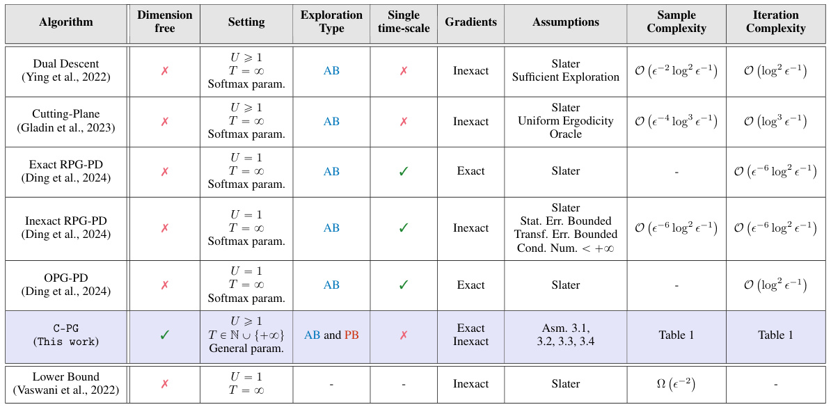
This table compares various primal-dual methods for constrained reinforcement learning, focusing on their ability to achieve last-iterate global convergence. It contrasts the algorithms across several key features: whether they are dimension-free (independent of state/action space size), the setting (number of constraints, infinite vs. finite horizon), the exploration type (action-based or parameter-based), whether they use single or multiple timescales for learning rate updates, whether they employ exact or inexact gradients, the assumptions needed for their convergence guarantees, and their sample and iteration complexity. The table also includes a lower bound on sample complexity for reference.

This table shows how different risk measures can be obtained by selecting the functions fi and gi in the unified risk measure formulation. It lists four risk measures: Expected Cost, Mean Variance, CVaRα, and Chance, along with their associated parameters (κ, α, η). For each risk measure, the table provides the specific form of the functions fi and gi, indicating whether a parameter η is needed and if a GPOMDP-like estimator is available. This table is crucial for understanding how the proposed algorithms can be applied to various risk-averse settings.

This table compares various primal-dual methods for constrained reinforcement learning, focusing on their ability to achieve last-iterate global convergence guarantees. It contrasts the methods across several key aspects: whether they are dimension-free (i.e., convergence rates do not depend on the problem’s dimension), the type of exploration paradigm used (action-based or parameter-based), whether they utilize a single or multiple time scales for updates, the type of gradients used (exact or inexact), the assumptions required for convergence guarantees, and their corresponding sample and iteration complexities. The table also notes the existence of a lower bound for sample complexity found in other research. It highlights the unique contributions of the proposed C-PG algorithm by comparing it to existing approaches.

This table compares various primal-dual methods for constrained reinforcement learning, focusing on their ability to achieve last-iterate global convergence. It contrasts algorithms’ dimension-free properties, single/multi-timescale nature, type of gradient used (exact or inexact), exploration paradigms (action-based or parameter-based), assumptions required for convergence, and the resulting sample and iteration complexities.

This table compares various primal-dual methods for constrained reinforcement learning, focusing on their ability to achieve last-iterate global convergence guarantees. It contrasts the algorithms across several key aspects: whether they are dimension-free, the type of constraints handled, the exploration paradigm used (action-based or parameter-based), if they operate on a single time scale, the type of gradients used (exact or inexact), the assumptions required for convergence, and the resulting sample and iteration complexities. The table also includes a lower bound on the sample complexity from existing research.

This table lists the parameters used for different risk measures in the Swimmer-v4 experiment using the C-PGAE algorithm. It shows the risk measure (Average Cost, CVaR, Mean Variance, Chance), the associated risk parameter (α, κ, n), the constraint threshold (b), and the learning rates used for the policy parameters (ζθ,0), dual variables (ζλ,0), and risk parameters (ζη,0). The ‘X’ indicates that a parameter is not needed for the corresponding risk measure.

This table lists the parameters used in the Swimmer-v4 experiment with the C-PGAE algorithm for different risk measures. It shows the risk measure (Average Cost, CVaR, Mean Variance, Chance), the corresponding risk parameter (κ, α, n), the constraint threshold (b), and the initial learning rates for the primal (ρ), dual (λ), and risk (η) variables. The initial learning rate for η is not used for Average Cost, as this risk measure does not depend on η.

This table shows the parameters used for different risk measures in the Swimmer-v4 experiment using the C-PGAE algorithm. It lists the risk measure (Average Cost, CVaR, Mean Variance, Chance), the corresponding risk parameter (κ, α, η), the constraint threshold (b), and the learning rates for the policy parameters (ζθ,0), the Lagrangian multipliers (ζλ,0), and the risk parameters (ζη,0). The table provides details for setting up the experiments, making it reproducible and highlighting the chosen parameters’ values.

This table shows the parameters used for the risk measures in the Swimmer-v4 experiment using the C-PGAE algorithm. It lists the risk measure (Average Cost, CVaRα, Mean Variance, Chance), the risk parameter (κ, α, η), the constraint threshold (b), and the learning rates (ζθ,0, ζλ,0, ζη,0). The values indicate specific settings used in the experiment.

This table compares several primal-dual methods for constrained reinforcement learning, focusing on their ability to achieve last-iterate global convergence. It contrasts various aspects, including whether the methods are dimension-free (independent of state and action space size), the type of policy gradient exploration used (action-based or parameter-based), whether they utilize a single or multiple time scales in their updates, the type of gradients (exact or inexact), the assumptions made for convergence guarantees, and the resulting sample and iteration complexities. The table also indicates whether the algorithm handles multiple constraints (U≥1) and the type of dual descent used.

This table compares several primal-dual methods for constrained reinforcement learning, focusing on their ability to guarantee last-iterate global convergence. It contrasts various aspects, including whether the method is dimension-free, the type of exploration used (action-based or parameter-based), single or multiple time scales, the type of gradient (exact or inexact), the assumptions required for convergence, and the resulting sample and iteration complexity. The table highlights the trade-offs between different approaches, particularly regarding computational efficiency and the strength of convergence guarantees.
Full paper#


