↗ OpenReview ↗ NeurIPS Homepage ↗ Chat
TL;DR#
Many machine learning models struggle with large and complex tabular datasets, unlike tree-based methods which are robust. Recent transformer-based in-context learners show promise but are limited by context size; memory scales quadratically with data size. This makes them unsuitable for larger datasets.
To address this, the researchers propose LoCalPFN, combining retrieval and fine-tuning. Retrieval uses k-Nearest Neighbours (kNN) to select a local context for each point; fine-tuning adapts the transformer to this subset, improving performance. LoCalPFN achieves state-of-the-art results on 95 datasets, surpassing even tuned tree-based models, demonstrating the effectiveness of their approach for scaling in-context learning in tabular data.
Key Takeaways#
Why does it matter?#
This paper is crucial because it tackles the scalability challenges of in-context learning (ICL) for tabular data, a pervasive problem in various fields. By proposing a novel approach that combines retrieval and fine-tuning, it significantly enhances the performance and applicability of ICL models for larger, more complex datasets, opening new avenues for research and development in this critical area. The findings are important for researchers working on large-scale tabular data analysis, providing a more efficient and effective alternative to existing methods. The demonstration of state-of-the-art results on a large benchmark dataset establishes the efficacy of this approach.
Visual Insights#

This figure demonstrates the limitations of TabPFN when dealing with complex datasets and introduces the proposed solution using k-NN. Panel (a) shows TabPFN failing to classify concentric circles even with the full dataset as context (underfitting). Panel (b) shows that using k-nearest neighbours as a local context significantly improves classification. Panel (c) shows that the performance of the k-NN approach remains stable across different numbers of neighbours (k) and consistently outperforms the full-context approach.

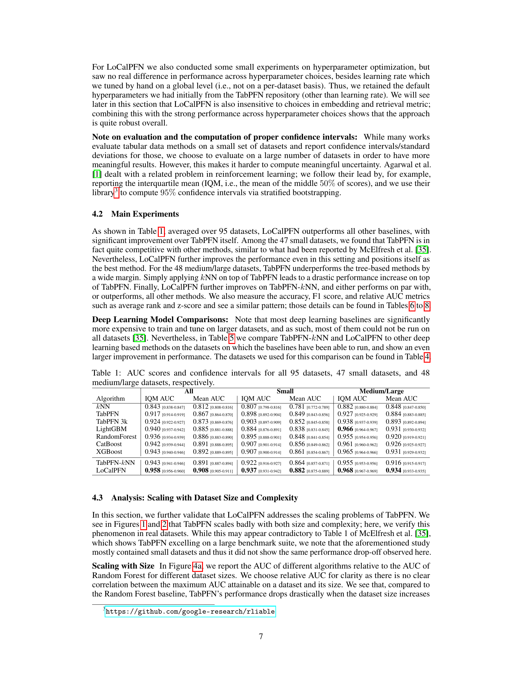
This table presents a comparison of the Area Under the ROC Curve (AUC) scores achieved by various algorithms on three different dataset sizes: all 95 datasets, 47 small datasets, and 48 medium/large datasets. For each algorithm and dataset size, it shows both the Interquartile Mean (IQM) AUC and the Mean AUC along with their corresponding 95% confidence intervals. The results highlight the performance of different algorithms across varying dataset complexities.
In-depth insights#
Tabular ICL Limits#
The heading ‘Tabular ICL Limits’ suggests an exploration of the boundaries and shortcomings of in-context learning (ICL) when applied to tabular data. A key limitation is the quadratic growth of memory requirements with context size. This directly impacts scalability, as larger datasets exceed available memory, hindering the application of ICL to more substantial real-world tabular datasets. The analysis likely investigates how this memory constraint affects model performance, potentially showing a degradation in accuracy or efficiency. Another potential limitation is the inherent lack of sequential structure in tabular data, unlike text or images. This absence of inherent order complicates the straightforward application of transformer-based ICL methods, which are designed to leverage sequential information. The exploration would likely compare the performance of ICL on tabular data with that of traditional machine learning techniques to highlight the relative strengths and weaknesses. The research may also delve into strategies to mitigate these limitations, such as employing efficient data retrieval techniques or modifying the ICL approach to better handle tabular data’s unique characteristics.
Retrieval Augment#
Retrieval augmentation, in the context of machine learning models, significantly enhances performance by incorporating external knowledge sources. This approach addresses limitations of traditional in-context learning, particularly when dealing with large or complex datasets. Instead of solely relying on the model’s internal parameters, retrieval augmentation leverages a separate knowledge base. When a query is received, relevant information is retrieved from this external source and combined with the input before feeding it to the model. This enriched input allows the model to make more informed and accurate predictions. The success of retrieval augmentation hinges on the effectiveness of the retrieval process and the model’s ability to integrate this retrieved information. Choosing the right retrieval method (e.g., keyword search, semantic similarity, k-NN) and incorporating the retrieved context properly is crucial. There are many applications for retrieval augmentation, but the core idea is to augment a core model’s capabilities by providing it with access to much larger amounts of data than can fit into its memory.
LoCalPFN: Method#
LoCalPFN, a novel approach to enhance in-context learning for tabular data, combines retrieval and fine-tuning to overcome limitations of existing methods like TabPFN. It leverages k-Nearest Neighbors (kNN) to retrieve a local subset of the data relevant to the query point, thus creating a context that adapts to the complexity of the data. This adaptive context is then used for end-to-end fine-tuning, further improving performance. This two-pronged strategy addresses TabPFN’s scaling issues by focusing computational resources on locally relevant data, thereby allowing efficient processing of larger and more complex datasets while maintaining high accuracy. The method is shown to achieve state-of-the-art results on extensive benchmarks, demonstrating the efficacy of combining retrieval and fine-tuning for improved in-context learning in tabular data settings.
Scaling & Tuning#
The heading ‘Scaling & Tuning’ suggests a focus on addressing limitations inherent in applying transformer-based in-context learning to tabular data. The core challenge lies in the quadratic growth of memory requirements with increasing dataset size, hindering the practical application of these methods to larger and more complex datasets. The paper likely proposes novel scaling techniques, perhaps involving retrieval methods (kNN) to focus the model’s attention on relevant subsets of data. Fine-tuning then becomes critical to further adapt the model to the specific characteristics of the retrieved subset, improving its performance for a given task. This combination likely achieves better scaling than vanilla in-context learning, allowing the model to handle significantly larger datasets. The tuning aspect would involve optimizing the model’s architecture, hyperparameters, and the interaction between retrieval and fine-tuning for maximal performance and efficiency. The successful implementation would demonstrate a significant advancement in scaling in-context learning for tabular data, improving its applicability to real-world problems that often involve massive datasets.
Future ICL Models#
Future In-Context Learning (ICL) models for tabular data hold immense potential. Addressing current limitations in scalability and complexity is paramount. This necessitates exploring more efficient context management techniques, potentially moving beyond simple k-NN retrieval to incorporate more sophisticated similarity measures or embedding spaces. Hybrid approaches, combining ICL with classical machine learning methods, such as tree-based models, could leverage the strengths of both paradigms. Research should focus on developing methods for automatically determining optimal context size and composition, adapting dynamically to the characteristics of each dataset. Investigating improved fine-tuning strategies tailored to the retrieved context is crucial for maximizing performance gains. Finally, the development of robust and versatile tabular foundation models, analogous to large language models, is vital for pushing the boundaries of ICL in tabular data analysis.
More visual insights#
More on figures

This figure shows how TabPFN and TabPFN-kNN perform with varying dataset sizes and context lengths. It demonstrates that TabPFN’s performance is limited by context size, hindering its ability to effectively use larger datasets. In contrast, TabPFN-kNN leverages k-NN to utilize larger datasets more efficiently, achieving improvements in performance even with shorter context lengths.

This figure illustrates the architecture and the efficient context used in LoCalPFN, which combines retrieval and fine-tuning. Panel (a) shows the overall architecture. During inference, the k-nearest neighbors (kNN) of a query point are used as its local context in the TabPFN model, which then predicts the query’s class. Panel (b) illustrates how this approach is modified for efficient fine-tuning. During fine-tuning, instead of using independent contexts for each query point, the model uses shared, local contexts by selecting a random training point, finding its kNNs, then randomly dividing them into context and query sets. This strategy allows for more efficient backpropagation and better scaling.

This figure illustrates the architecture and efficient context computation of LoCalPFN during both inference and fine-tuning. (a) shows the inference process: for each query point, the k-nearest neighbors (kNNs) are retrieved and used as context. (b) depicts the modified fine-tuning process: many queries share a local context by randomly sampling training points, computing their kNNs, and then randomly splitting these neighbors into context and query sets. This approach makes fine-tuning computationally more efficient.

This figure demonstrates the limitations of TabPFN in handling complex patterns with full context and how using a k-Nearest Neighbors (kNN) approach with adaptive local context improves performance. Panel (a) shows TabPFN’s underfitting when using the entire dataset as context, failing to classify concentric circles. Panel (b) illustrates how using kNN solves the problem. Panel (c) shows that the kNN method’s performance is robust to the number of neighbors (k) and consistently outperforms the full-context TabPFN approach.

This figure demonstrates the limitations of TabPFN (a) when using the full training dataset as context, especially for complex classification tasks. It then shows how using k-Nearest Neighbors (kNN) to create a local context for each data point dramatically improves performance (b), making the model robust to the complexity of the data even with varying numbers of neighbors (c).

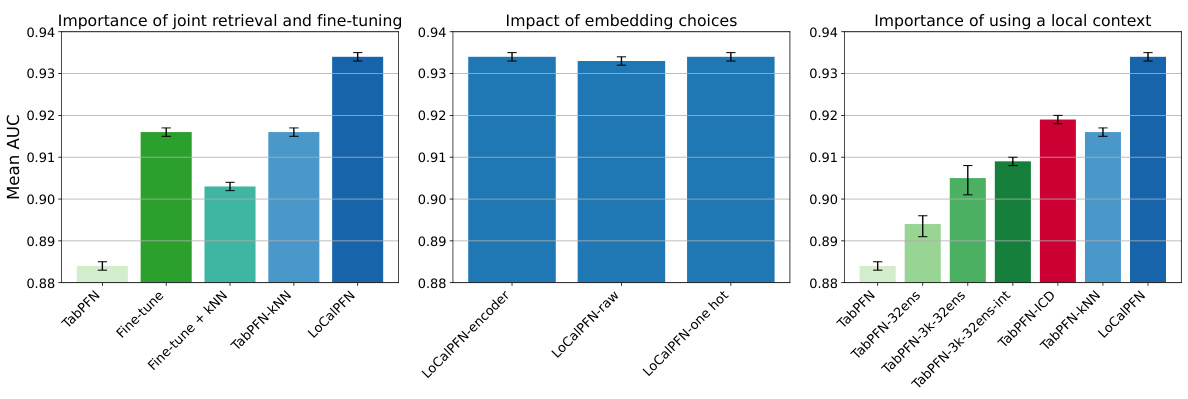
This figure shows the ablation study on the maximum number of neighbors used as context. The results show that TabPFN-kNN and LoCalPFN are not very sensitive to this choice as long as it is at least 100. LoCalPFN is able to improve TabPFN-kNN on all context sizes. Surprisingly, LoCalPFN outperforms the random forest baseline using a maximum context size of only 50 and also outperforms the XGBoost baseline with maximum context size of 500.

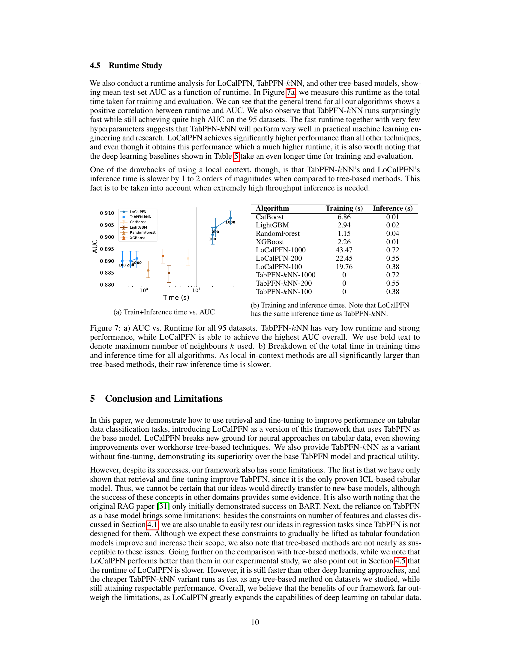
Figure 7 shows the relationship between runtime and performance (AUC) for various algorithms across 95 datasets. Panel (a) displays the total runtime (training + inference) against AUC. It highlights that TabPFN-kNN offers a remarkably low runtime while still achieving strong AUC scores, while LoCalPFN attains the highest AUC. Panel (b) provides a breakdown of the training and inference times for each algorithm. The figure demonstrates that while local in-context learning methods like TabPFN-kNN and LoCalPFN might exhibit higher inference times due to their nature, their overall performance and, in some cases, training time efficiency is still competitive.

This figure compares the performance of TabPFN with and without using k-Nearest Neighbors (kNN) for context adaptation. Panel (a) shows TabPFN failing to classify a simple pattern using full context. Panel (b) demonstrates successful classification using the kNN method with an adaptive local context. Panel (c) illustrates the robustness of the kNN approach across various numbers of neighbors (k) and demonstrates that kNN consistently outperforms TabPFN when using full context.
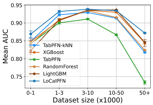
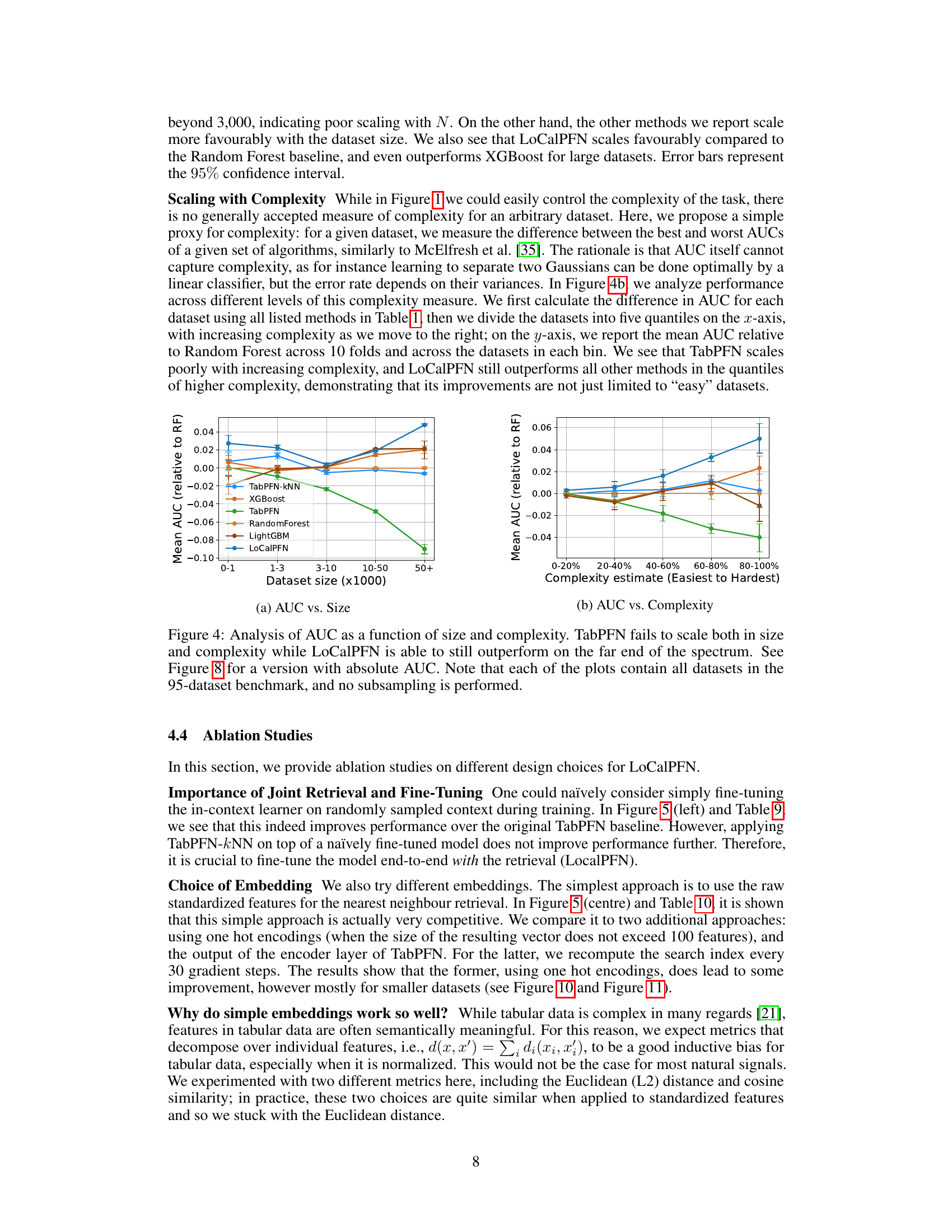
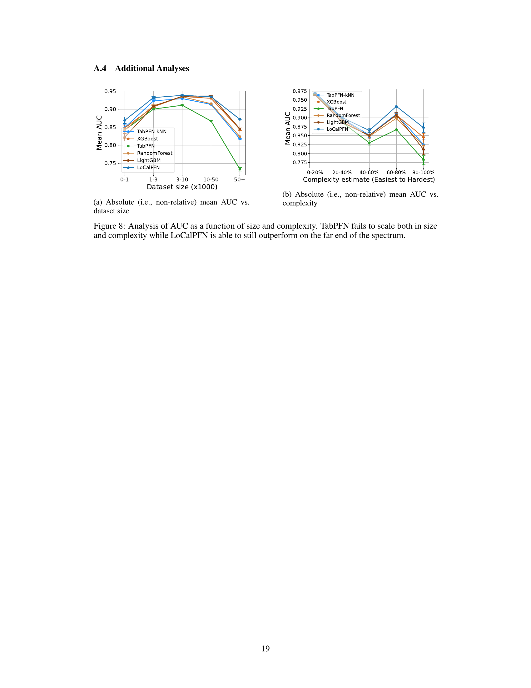
This figure analyzes the performance of different algorithms (TabPFN, LoCalPFN, XGBoost, Random Forest, LightGBM) across datasets of varying sizes and complexities. The x-axis represents dataset size (in thousands of instances) binned into categories (0-1, 1-3, 3-10, 10-50, 50+), and the y-axis shows the mean AUC (Area Under the Curve). The plot demonstrates that TabPFN’s performance degrades significantly as dataset size and complexity increase, unlike the other algorithms. LoCalPFN consistently outperforms all other methods, especially in larger, more complex datasets. Figure 8 provides the same information but displays the absolute AUC scores instead of relative AUC scores.

This figure shows the limitations of TabPFN when using the full dataset as context and how a local context approach (using k-NN) improves its performance on a synthetic dataset with increasing complexity. (a) shows the underfitting of TabPFN with full context on a dataset with three concentric circles. (b) shows how the local context approach resolves the underfitting problem. (c) demonstrates the robustness of the k-NN method to different numbers of neighbors and its superiority over TabPFN with full context for various dataset complexities.
This figure demonstrates the limitations of TabPFN (a transformer-based in-context learner) when dealing with complex tabular data and introduces a solution using k-Nearest Neighbors (kNN). Panel (a) shows TabPFN failing to classify simple concentric circles using the full dataset as context, highlighting its underfitting. Panel (b) showcases the improved performance using kNN to provide a localized context for each data point. Panel (c) demonstrates the robustness of the kNN approach across varying k values and dataset complexities, consistently outperforming the vanilla TabPFN method.
This figure shows that TabPFN underfits when using the entire training dataset as context, failing to classify complex patterns (Figure 1a). Using k-Nearest Neighbors (kNN) to provide a local context for each point improves classification significantly (Figure 1b). Figure 1c demonstrates that the kNN-based approach remains robust to changes in the number of neighbors (k) even with increasing dataset complexity, outperforming the vanilla TabPFN using the full context.
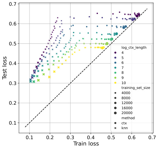
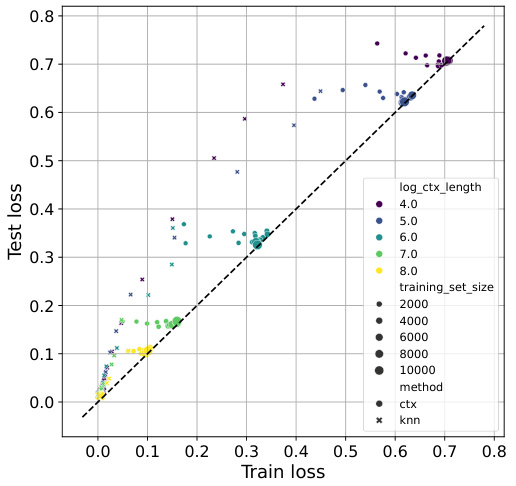
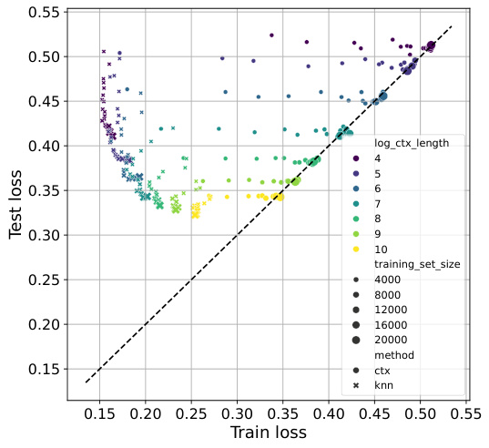
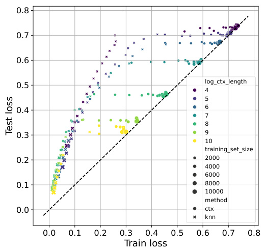
This figure displays the relationship between training loss and test loss for TabPFN and TabPFN-kNN across four datasets with varying dataset sizes and context lengths (number of neighbors). It demonstrates how TabPFN-kNN offers better control over overfitting/underfitting, particularly with smaller datasets and fewer neighbors.
This figure compares the performance of TabPFN with and without using k-Nearest Neighbors (kNN) for context adaptation. Panel (a) shows TabPFN’s failure to classify complex patterns using the full dataset as context, highlighting the underfitting issue. Panel (b) demonstrates how using kNN improves performance by providing an adaptive local context for each data point. Finally, panel (c) showcases the robustness and consistent superiority of the kNN approach across different k values and increasing dataset complexity.

This figure shows the limitations of TabPFN when using the full dataset as context and proposes a solution using k-NN to adapt the transformer to local subsets of data. (a) demonstrates TabPFN’s underfitting on concentric circles; (b) shows the improvement with k-NN; and (c) compares the performance of the two methods across different dataset complexities.
This figure shows the limitations of TabPFN when dealing with complex datasets. Panel (a) demonstrates TabPFN’s underfitting, failing to classify simple concentric circles when using its full context. Panel (b) showcases the improved performance of using k-Nearest Neighbors (kNN) to create a local context for each data point, enabling accurate classification. Panel (c) shows the robustness of this kNN-based approach to the number of neighbors (k) and its consistent outperformance of the vanilla TabPFN across varying dataset complexities.
More on tables

This table presents a comparison of the Area Under the Curve (AUC) scores achieved by various algorithms on different datasets. It breaks down the results by dataset size (all datasets, small datasets, and medium/large datasets) and includes confidence intervals to indicate the reliability of the results. The algorithms compared include KNN, TabPFN, TabPFN-3k, LightGBM, RandomForest, CatBoost, XGBoost, TabPFN-kNN, and LoCalPFN. This comparison allows for an assessment of the relative performance of each algorithm across diverse datasets.
This table presents a comparison of the Area Under the Curve (AUC) scores achieved by various algorithms on three different dataset sizes: all 95 datasets, 47 small datasets, and 48 medium/large datasets. The AUC is a common metric for evaluating the performance of classification models. The table shows the Interquartile Mean (IQM) AUC and the mean AUC, along with 95% confidence intervals, for each algorithm and dataset size. This allows for a comprehensive comparison of the algorithms’ performance across different dataset scales and complexities.
This table presents the Area Under the Curve (AUC) scores and their corresponding 95% confidence intervals for three different dataset sizes: all 95 datasets, 47 small datasets, and 48 medium/large datasets. The AUC is a common metric for evaluating the performance of classification models, providing a measure of how well the model can distinguish between different classes. The confidence intervals give a range within which the true AUC is likely to fall, reflecting the uncertainty in the estimated score due to the limited sample size of the datasets. The table allows for a comparison of LoCalPFN and other machine learning algorithms across various dataset sizes and difficulties.
This table presents a comparison of the Area Under the Curve (AUC) scores achieved by various algorithms on three dataset groups: all 95 datasets, 47 small datasets, and 48 medium/large datasets. The AUC is a metric for evaluating the performance of binary classification models. The table includes the Interquartile Mean (IQM) AUC and the range of the 95% confidence intervals for each algorithm, offering a comprehensive view of the model performance across different dataset sizes and complexities.

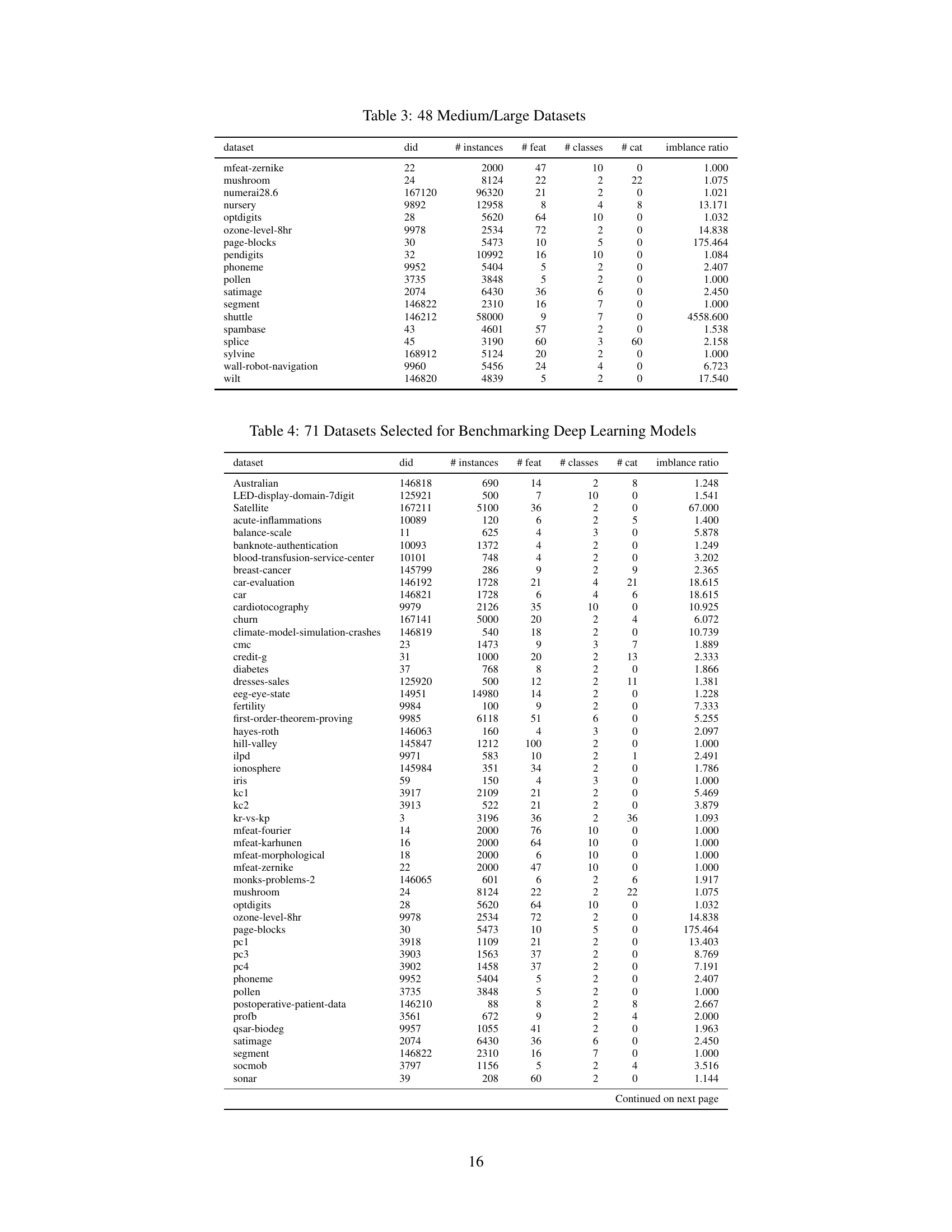
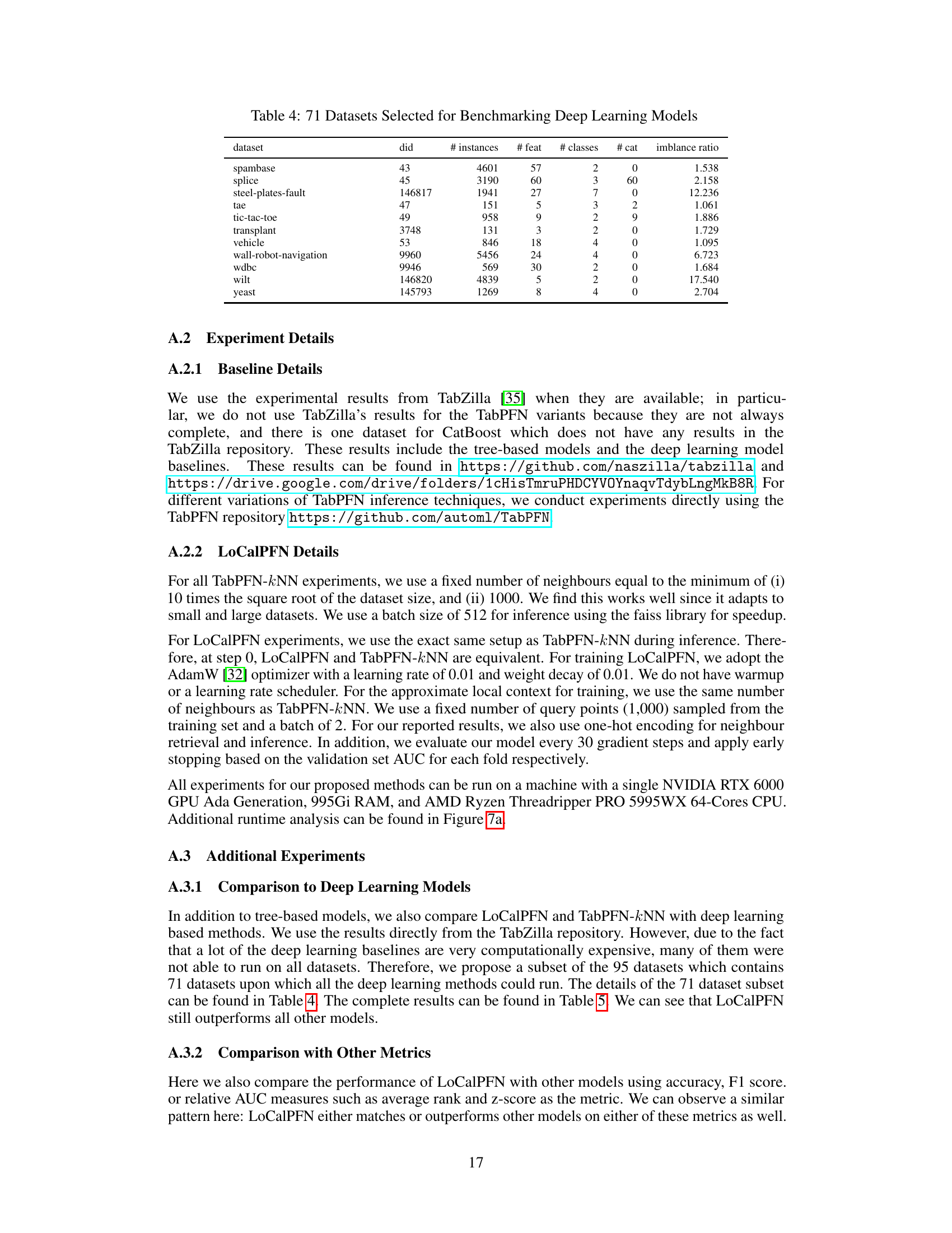
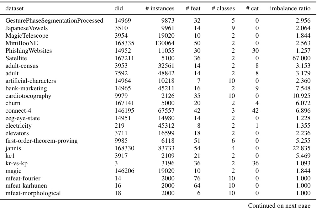
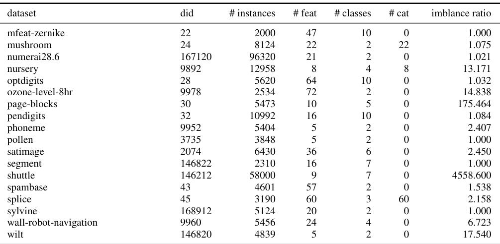
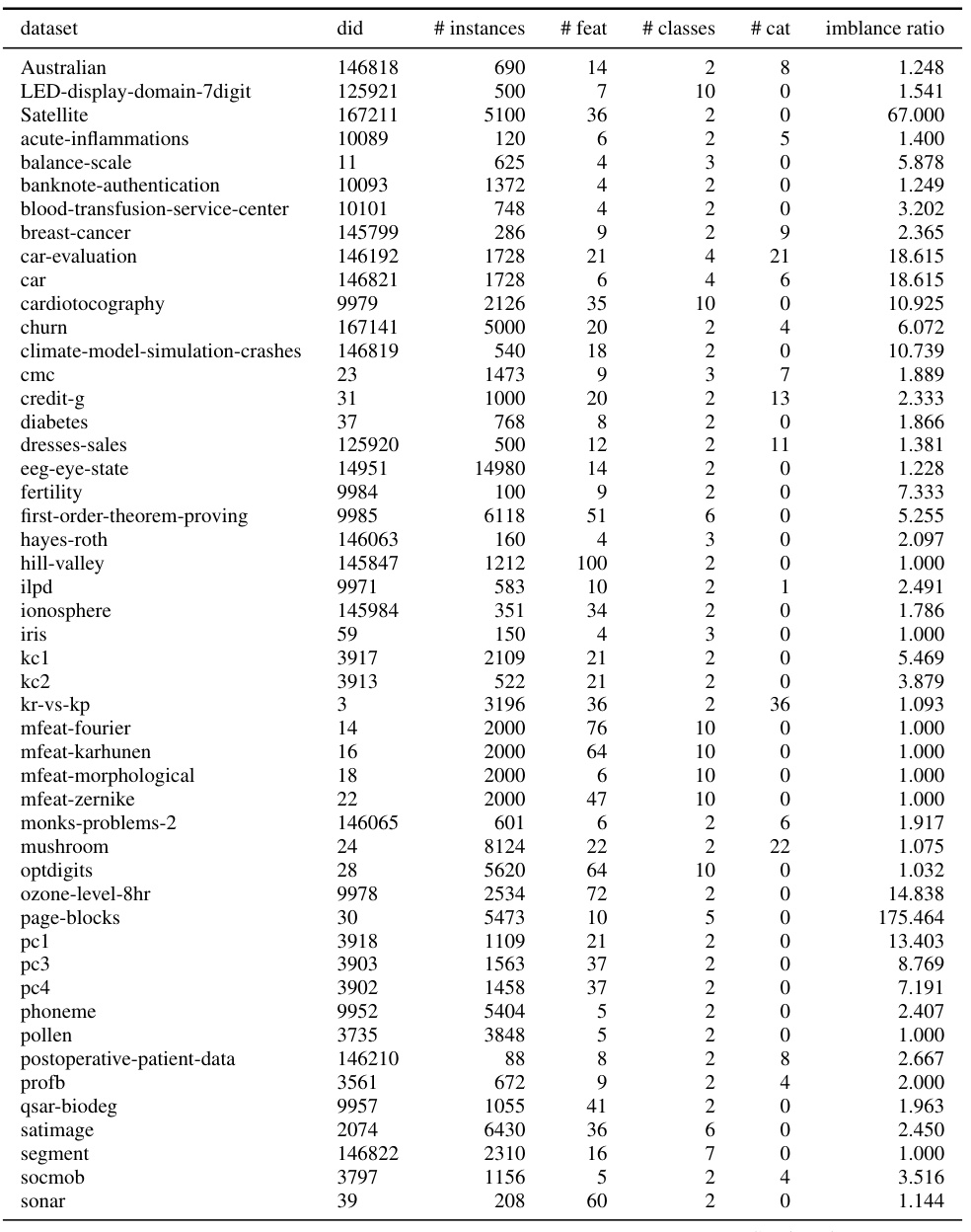
This table lists 71 datasets used for benchmarking deep learning models in the paper. For each dataset, it provides the dataset ID from OpenML, the number of instances, the number of features, the number of classes, the number of categorical features, and the imbalance ratio. This subset of datasets was chosen to ensure that all deep learning models included in the comparison could run on them, unlike the full set of 95 datasets which contained larger datasets that were computationally prohibitive for some methods.
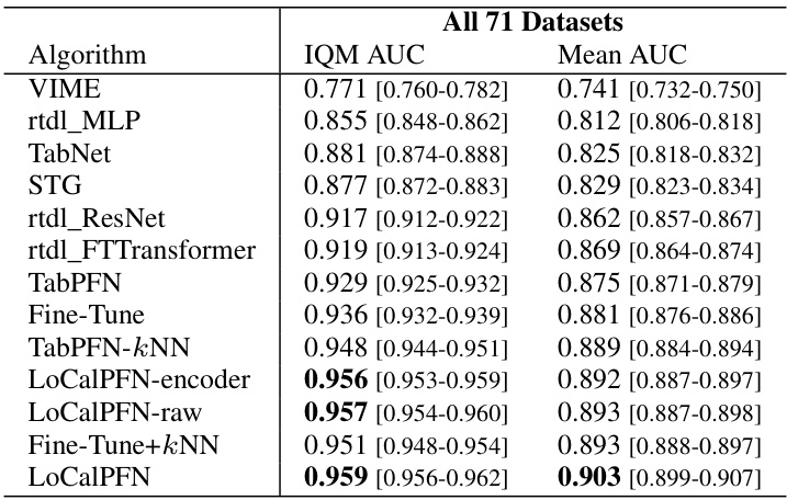
This table presents the Area Under the Curve (AUC) scores and their corresponding 95% confidence intervals for different machine learning algorithms. The algorithms are evaluated on three dataset sizes: all 95 datasets, 47 small datasets, and 48 medium/large datasets. The results provide a quantitative comparison of the performance of various algorithms across different dataset sizes, highlighting their strengths and weaknesses in handling tabular data of varying complexity and scale.

This table presents the Area Under the Curve (AUC) scores and their corresponding 95% confidence intervals for the LoCalPFN model and several baseline models. The results are broken down for all 95 datasets, as well as separately for 47 smaller datasets and 48 medium/large datasets, to illustrate performance variation based on dataset size.

This table presents a comparison of the Area Under the Curve (AUC) scores achieved by various algorithms on three different dataset sizes: all 95 datasets, 47 small datasets, and 48 medium/large datasets. The AUC is a common metric for evaluating the performance of classification models. For each algorithm and dataset size, the table shows the Interquartile Mean (IQM) AUC and the 95% confidence interval. The IQM AUC provides a robust estimate of the central tendency of the AUC scores, while the confidence interval indicates the uncertainty associated with the estimate.
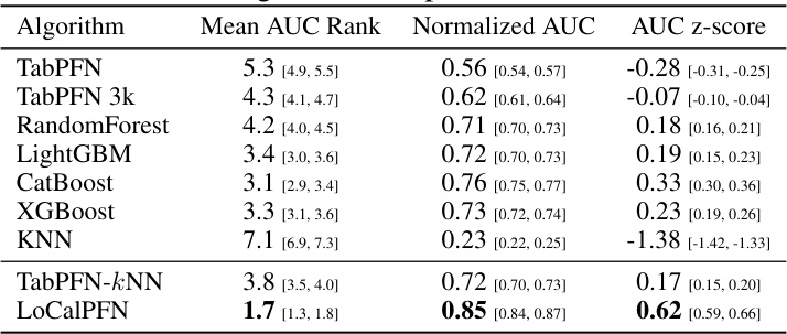
This table presents the Area Under the Curve (AUC) scores and their corresponding 95% confidence intervals for different machine learning algorithms. The algorithms are evaluated on three groups of datasets: all 95 datasets, 47 small datasets, and 48 medium/large datasets. The results showcase the performance comparison of various algorithms, highlighting the differences in their accuracy across different dataset sizes and complexities.

This table presents a comparison of the Area Under the Curve (AUC) scores achieved by different algorithms on three dataset groups: all 95 datasets, 47 small datasets, and 48 medium/large datasets. The AUC metric is a common measure of classifier performance, indicating the probability that a randomly chosen positive instance will be ranked higher than a randomly chosen negative instance. For each algorithm and dataset group, the table reports both the interquartile mean (IQM) of the AUC scores and the corresponding 95% confidence interval. The IQM is used because it is more robust to outliers compared to the traditional mean. The confidence intervals provide an indication of the uncertainty in the AUC estimates. The table allows for the evaluation of the relative performance of different algorithms on datasets of varying sizes and complexities.

This table presents the Area Under the Curve (AUC) scores and their corresponding 95% confidence intervals for the LoCalPFN model and several baseline models across three dataset groups: all 95 datasets, 47 small datasets, and 48 medium/large datasets. The AUC score is a measure of the model’s ability to distinguish between classes. The confidence intervals provide a range within which the true AUC score is likely to fall. This allows for comparison of the performance of different models on datasets of various sizes and complexities.

This table presents the Area Under the Curve (AUC) scores and their corresponding 95% confidence intervals for various algorithms evaluated on three different dataset sizes: all 95 datasets, 47 small datasets, and 48 medium/large datasets. The algorithms include kNN, TabPFN, TabPFN-3k, LightGBM, RandomForest, CatBoost, XGBoost, TabPFN-kNN, and LoCalPFN. The results show a comparison of performance across different algorithms and dataset sizes, highlighting the relative strengths and weaknesses of each approach under varying conditions.
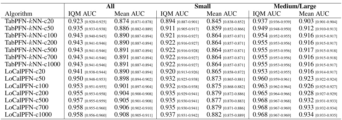
This table presents the Area Under the Curve (AUC) scores and their corresponding 95% confidence intervals for various algorithms across three different dataset sizes: all 95 datasets, 47 small datasets, and 48 medium/large datasets. The algorithms compared include several tree-based methods (Random Forest, LightGBM, CatBoost, XGBoost) and several deep learning methods (KNN, TabPFN, TabPFN-kNN, LoCalPFN). The table allows for a comparison of the performance of different algorithms across various dataset sizes and helps to determine the best performing algorithm for each dataset size category.

This table presents a comparison of the Area Under the Curve (AUC) scores achieved by different algorithms on three dataset groups: all 95 datasets, 47 small datasets, and 48 medium/large datasets. For each algorithm and dataset group, the table shows the Interquartile Mean (IQM) AUC and the 95% confidence interval. The algorithms compared include KNN, TabPFN, TabPFN-3k, LightGBM, RandomForest, CatBoost, XGBoost, TabPFN-kNN, and LoCalPFN. The results demonstrate the superior performance of LoCalPFN across all dataset groups compared to other methods.
Full paper#
