↗ OpenReview ↗ NeurIPS Homepage ↗ Chat
TL;DR#
The dominance of gradient-boosted decision trees for classification and regression on tabular data is challenged by deep learning methods, often hampered by slow training and extensive hyperparameter tuning. This research introduces RealMLP, an enhanced MLP, and provides well-tuned default parameters for both RealMLP and GBDTs. This addresses the discrepancy between deep learning and traditional methods in terms of speed and ease of use.
The proposed RealMLP model, along with the new default parameters, demonstrates favorable time-accuracy tradeoffs. The meta-tuned parameters show that RealMLP and GBDTs, can achieve excellent results without any hyperparameter optimization, thereby significantly reducing computational costs and time for practitioners and researchers. The improved default parameters also enhance the performance of existing TabR models.
Key Takeaways#
Why does it matter?#
This paper is crucial for researchers in machine learning and data science due to its focus on improving the performance of both deep learning models and gradient boosted decision trees (GBDTs) on tabular data without extensive hyperparameter tuning. It provides well-tuned default parameters that save significant time and effort, thereby enhancing the usability of these models for a wider range of applications and practitioners.
Visual Insights#

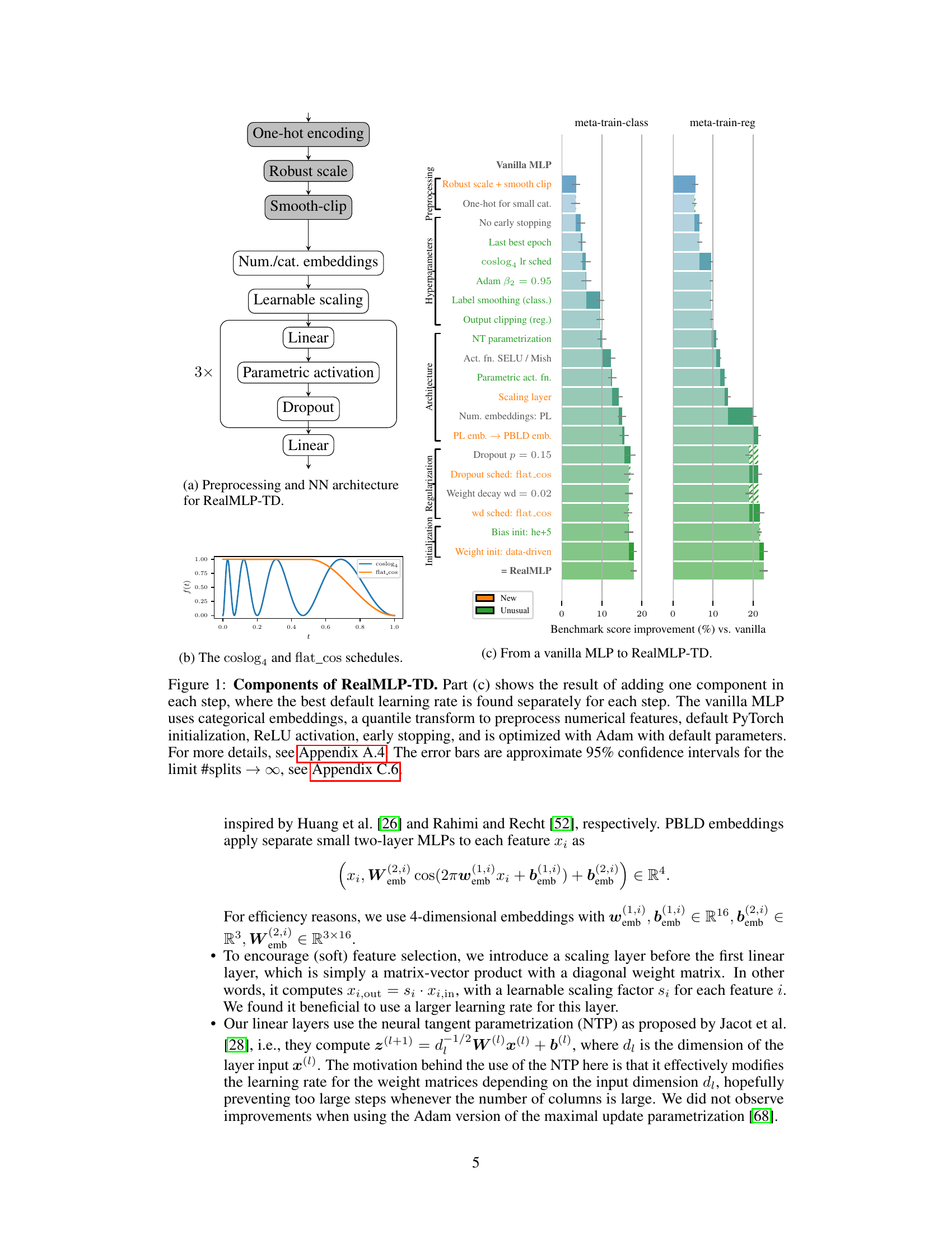
This figure illustrates the architecture of RealMLP-TD, a novel multilayer perceptron (MLP) designed for tabular data. Panel (a) shows the preprocessing steps and the MLP architecture, including details such as one-hot encoding for categorical features, robust scaling and smooth clipping for numerical features, and the use of learnable scaling and parametric activation functions. Panel (b) displays the learning rate schedules used. Finally, panel (c) shows a cumulative ablation study where the effect of incrementally adding each component to a vanilla MLP on the benchmark score is presented.

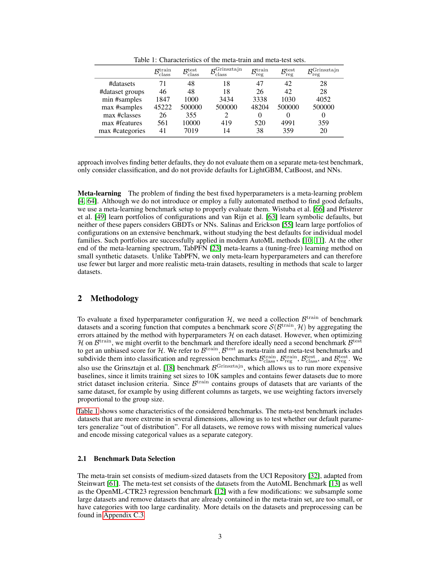
This table presents a comparison of the characteristics of the meta-train and meta-test datasets used in the paper. The meta-train set was used for optimizing the default hyperparameters of the models, while the meta-test set was used for evaluating the performance of the models with these optimized hyperparameters. The table shows the number of datasets, dataset groups, minimum and maximum number of samples, maximum number of classes, maximum number of features, and maximum number of categories for each dataset split (meta-train and meta-test, classification and regression). The Grinsztajn et al. (2022) benchmark is also included for comparison.
In-depth insights#
Tuned Defaults Win#
The concept of “Tuned Defaults Win” in a machine learning research paper suggests that carefully optimized default hyperparameters can significantly outperform models relying on extensive hyperparameter optimization (HPO). This challenges the conventional wisdom that HPO is always necessary for achieving state-of-the-art results. The key insight lies in meta-learning, where default settings are tuned across a diverse set of datasets, effectively learning dataset-agnostic parameters. This approach offers a favorable time-accuracy tradeoff because it avoids the computationally expensive process of HPO for every single dataset. The results likely demonstrate that well-tuned defaults, achieved through rigorous meta-learning, provide a robust and efficient alternative to HPO, particularly beneficial when considering deployment in real-world applications where the computational cost of HPO is a significant constraint. The research probably also includes a detailed analysis comparing the performance of models with tuned defaults against those using HPO, showing comparable or even superior results in many instances, thereby highlighting the practical importance of this approach. The paper likely emphasizes the generalizability of the tuned defaults, indicating their effectiveness across unseen datasets beyond the meta-training set. The practical implications are substantial, potentially paving the way for more efficient and accessible AutoML systems.
RealMLP’s Tricks#
The RealMLP architecture incorporates several “tricks” to improve performance on tabular data. Robust scaling and smooth clipping preprocess numerical features, handling outliers effectively. A novel numerical embedding, PBLD (periodic bias linear DenseNet), combines the original feature value with periodic embeddings and biases, potentially capturing both linear and non-linear relationships. A diagonal weight layer allows for learnable feature scaling, enabling soft feature selection. Careful hyperparameter tuning, including the use of a multi-cycle learning rate schedule and parametric activation functions, further enhances performance. These techniques, while not revolutionary individually, demonstrate that combining well-chosen, non-standard techniques yields substantial improvements in performance and time efficiency on tabular datasets compared to traditional MLPs and can even compete with GBDTs.
Benchmark Tradeoffs#
Analyzing benchmark tradeoffs in machine learning research is crucial for responsible model selection. A thoughtful approach should consider time-accuracy tradeoffs, acknowledging that faster models might sacrifice some accuracy, and vice-versa. This involves comparing models across multiple benchmark datasets, realizing that no single model universally outperforms others. The analysis must account for dataset characteristics such as size, dimensionality, and feature types, since model performance can significantly vary depending on these factors. Evaluation metrics, beyond simple accuracy, should be employed for regression and classification tasks. Statistical significance tests need to be incorporated to confirm the reliability of observed differences, and proper error bars must be reported. Furthermore, it’s important to assess the impact of hyperparameter tuning, recognizing that extensive tuning can lead to overfitting specific benchmarks and hinder generalizability. Finally, it’s necessary to critically evaluate the computational resources required, ensuring that benchmark comparisons aren’t skewed by the availability of high-end hardware.
Meta-Learning HPO#
Meta-learning applied to hyperparameter optimization (HPO) represents a significant advancement in automating machine learning model selection and training. Instead of tuning hyperparameters on a per-dataset basis, meta-learning HPO aims to learn generalizable strategies for hyperparameter selection across diverse datasets. This is achieved by training a meta-learner on a large collection of datasets, enabling it to predict optimal hyperparameters for new, unseen datasets based on their characteristics. The core advantage is the potential for substantial time savings, eliminating the need for extensive and often computationally expensive dataset-specific HPO. However, the effectiveness of meta-learning HPO critically depends on the quality and diversity of the meta-training data. A biased or insufficient meta-training dataset can lead to suboptimal performance and generalization failure. Furthermore, the meta-learner itself introduces another layer of complexity, requiring its own hyperparameter tuning and careful design. Despite these challenges, meta-learning HPO demonstrates promising results in achieving excellent performance with minimal manual intervention, potentially revolutionizing the way machine learning models are developed and deployed.
Future of Tabular ML#
The future of tabular ML is bright, driven by several key trends. Deep learning’s impact will likely increase, but not necessarily replace traditional methods like gradient-boosted decision trees (GBDTs). We’ll see more hybrid models combining the strengths of both approaches, leveraging deep learning’s ability to learn complex relationships and GBDTs’ efficiency and interpretability. Improved default parameters and automated machine learning (AutoML) will play crucial roles, making sophisticated methods more accessible. The development of more robust and generalizable benchmarks is also vital, ensuring fairness and enabling comparison across diverse methods and datasets. Finally, we’ll see ongoing research in feature engineering, and addressing issues like high-cardinality features and missing data with more innovative solutions. This will focus on making models more resilient to challenges found in real-world tabular datasets.
More visual insights#
More on figures
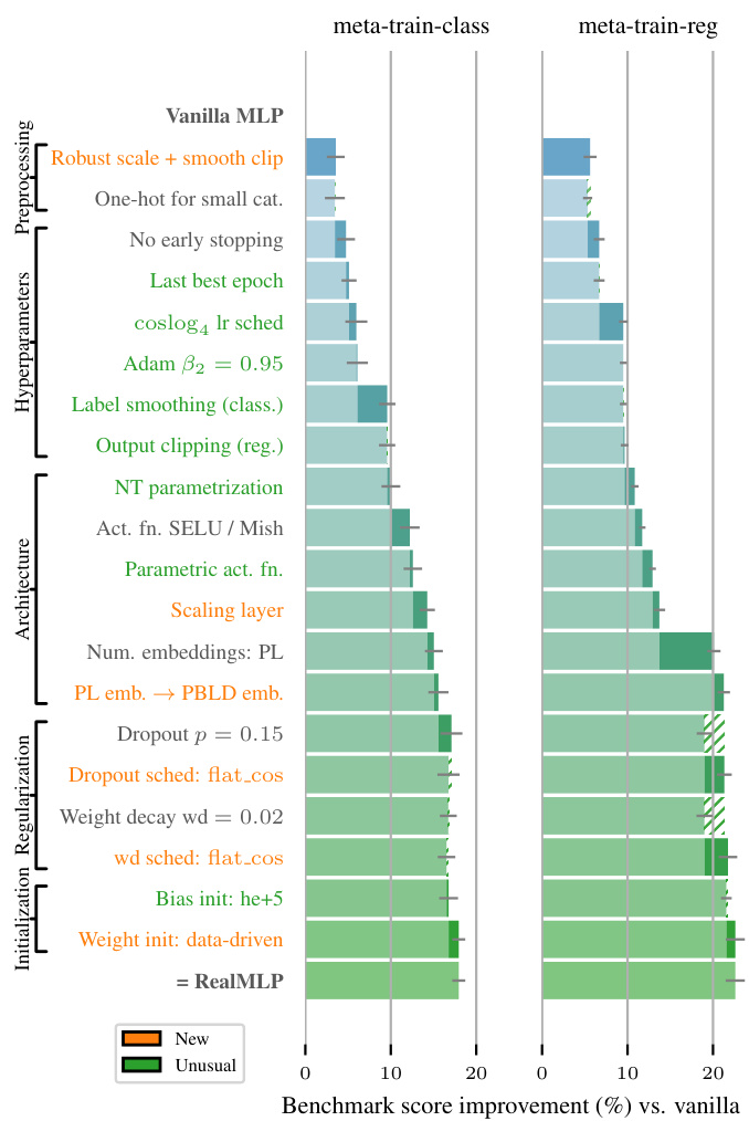
This figure details the components of RealMLP-TD, an improved multilayer perceptron (MLP) with tuned default parameters. Part (a) illustrates the preprocessing steps and NN architecture of RealMLP-TD. Part (b) shows the learning rate schedules used (coslog4 and flat_cos). Part (c) shows a cumulative ablation study, demonstrating the individual contribution of each component to the overall performance improvement compared to a vanilla MLP. The study measures improvements on a meta-train benchmark. Error bars represent approximate 95% confidence intervals.

This figure shows the architecture and the training process for RealMLP-TD, a novel Multilayer Perceptron (MLP) for tabular data. Part (a) details the preprocessing steps and the MLP architecture, including components such as categorical embeddings, numerical embeddings (PL and PBLD), a learnable scaling layer, parametric activation functions, and dropout. Part (b) illustrates the learning rate schedules (coslog4 and flat_cos) used during training. Part (c) presents a cumulative ablation study, demonstrating the impact of each component on the model’s performance as compared to a vanilla MLP. The results highlight the effectiveness of the various design choices in improving RealMLP-TD’s accuracy and efficiency.

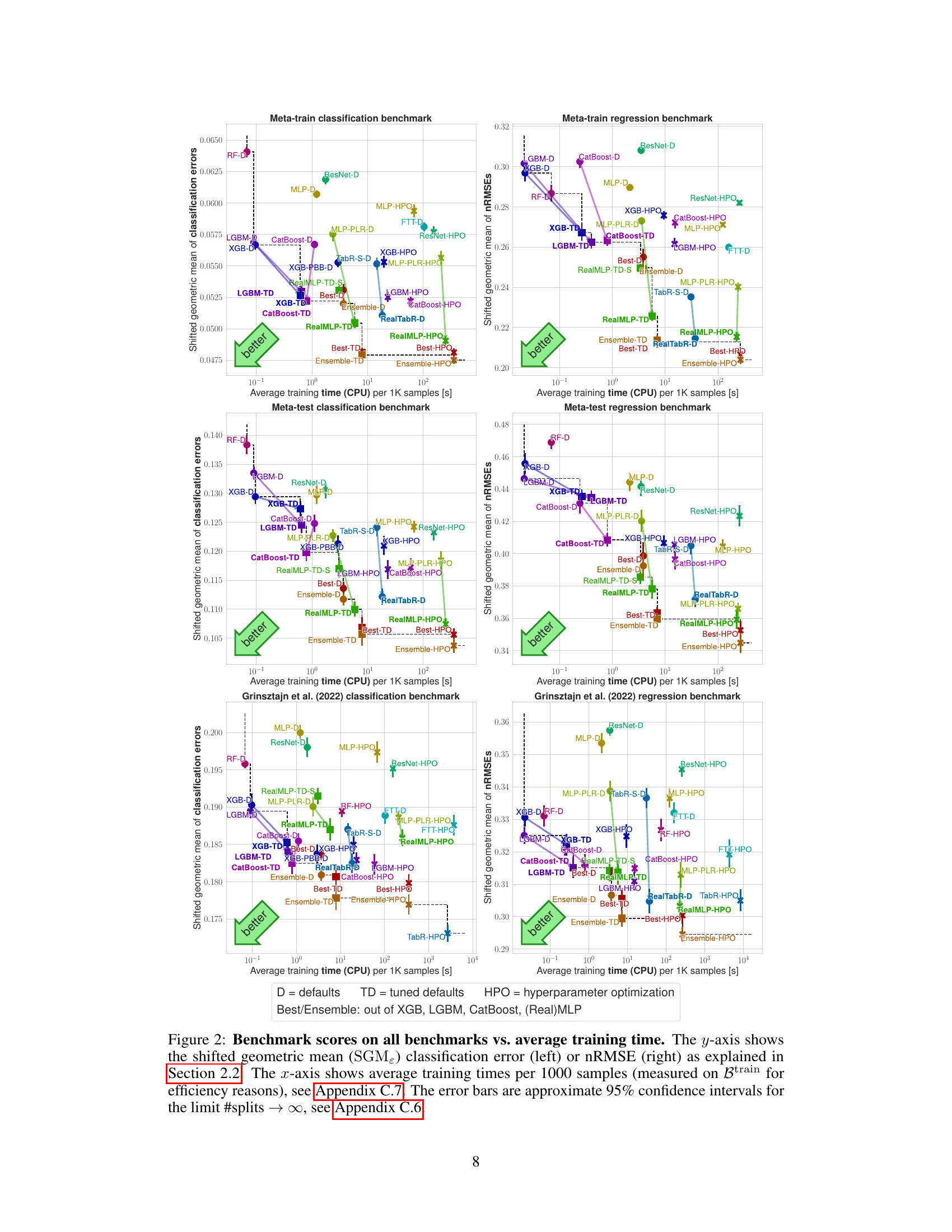
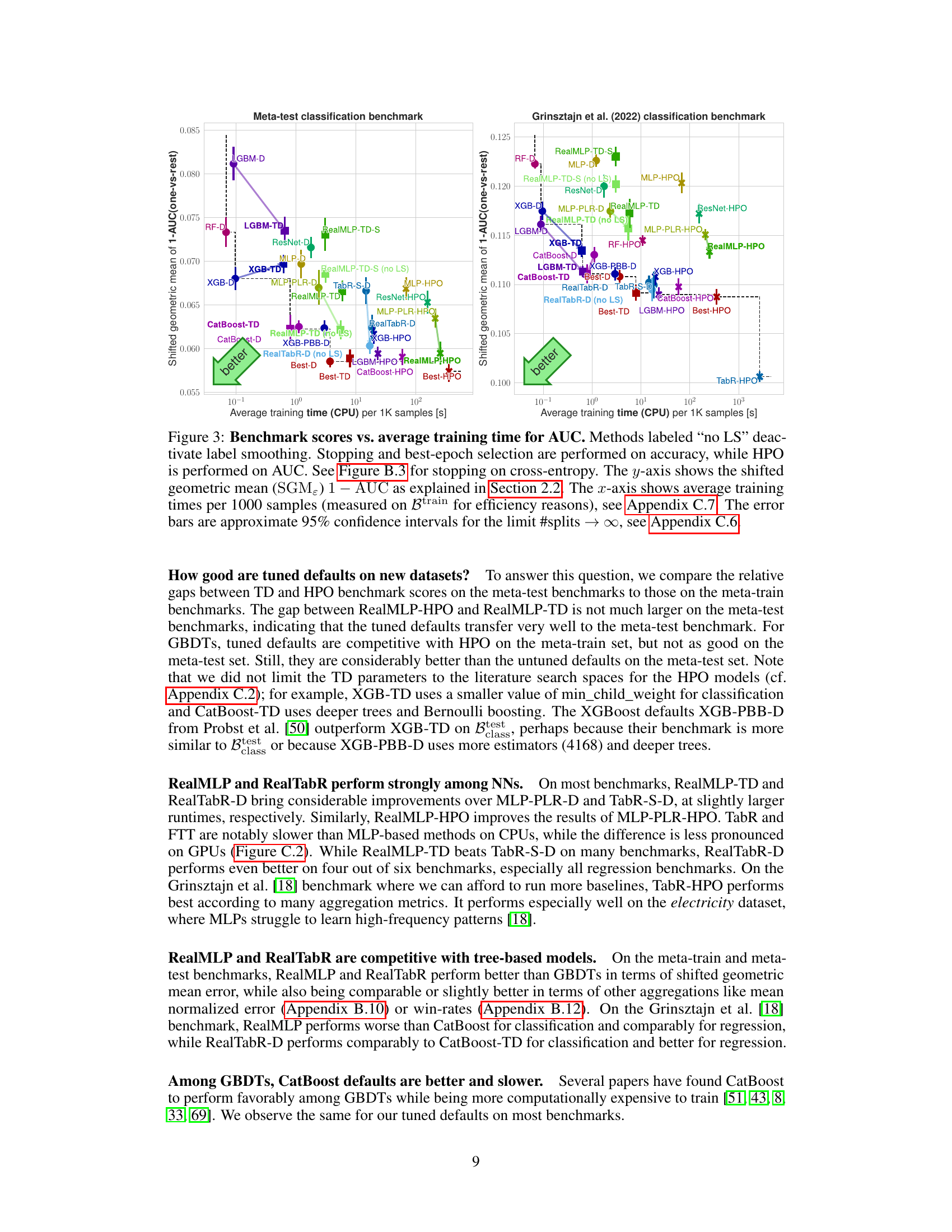
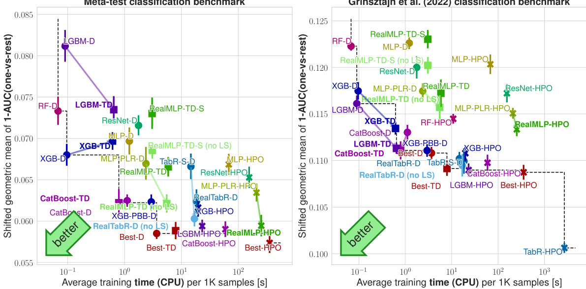
This figure compares multiple machine learning models on various benchmark datasets. The y-axis represents the model performance (classification error or nRMSE, as explained in section 2.2 of the paper) using a shifted geometric mean across multiple test-train splits. The x-axis indicates the average training time per 1000 samples. Each point in the figure shows the performance and training time of a particular method on the specified benchmarks, with error bars representing approximate 95% confidence intervals. Different colors are used to denote different model types (GBDTs, NNs, etc.) and parameter settings (library defaults, tuned defaults, hyperparameter optimization). The figure enables a direct comparison of the tradeoff between speed and accuracy for various algorithms on different datasets.
This figure compares various machine learning models on four different benchmarks (meta-train classification, meta-train regression, meta-test classification, meta-test regression) and shows the tradeoff between their accuracy (y-axis) and training time (x-axis). The y-axis uses the shifted geometric mean to aggregate the error across multiple datasets. The x-axis displays average training time per 1000 samples (on the meta-training dataset). Each point represents one model, and error bars provide an estimate of the uncertainty.

This figure compares different machine learning models’ performance across multiple benchmark datasets. The y-axis represents the model’s error rate (classification error or normalized root mean squared error), calculated using a modified geometric mean to account for datasets with zero error. The x-axis shows the training time for the models, normalized to the time taken to process 1000 data samples. The graph allows for a direct comparison of models’ time-accuracy trade-offs. Error bars represent the 95% confidence interval, illustrating the reliability of the measured error rates.

This figure compares various machine learning models’ performance across multiple benchmarks. The y-axis represents the model’s accuracy (classification error or nRMSE), using a shifted geometric mean to aggregate results across datasets and multiple random train-test splits. The x-axis displays the average training time per 1000 samples, measured on the meta-train dataset for efficiency. Error bars indicate approximate 95% confidence intervals, accounting for variability across multiple random splits. Different colors represent different algorithms, including various gradient-boosted decision trees (GBDTs) and neural networks (NNs), with and without hyperparameter optimization (HPO). The figure helps to illustrate the time-accuracy tradeoff of each algorithm and the effect of hyperparameter tuning on the overall performance.
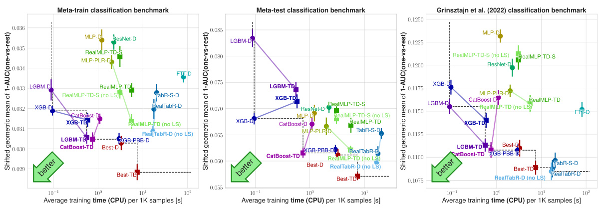
This figure compares various machine learning models on different benchmark datasets in terms of their time-accuracy tradeoff. The y-axis represents the performance, measured as shifted geometric mean classification error or normalized root mean squared error (nRMSE). The x-axis shows the average training time per 1000 samples. Each point represents a specific model and its performance on a given dataset. Error bars indicate the 95% confidence interval, showing the uncertainty. The plot aims to visualize which models offer a favorable balance between computational cost and prediction accuracy.

This figure compares multiple machine learning models across different benchmark datasets, showing their performance (classification error or nRMSE) against their training time. The y-axis represents the shifted geometric mean error, a metric designed to be less sensitive to outliers than other aggregation metrics. The x-axis shows average training time per 1000 samples, measured on a specific subset of the training data for efficiency. The error bars represent 95% confidence intervals.
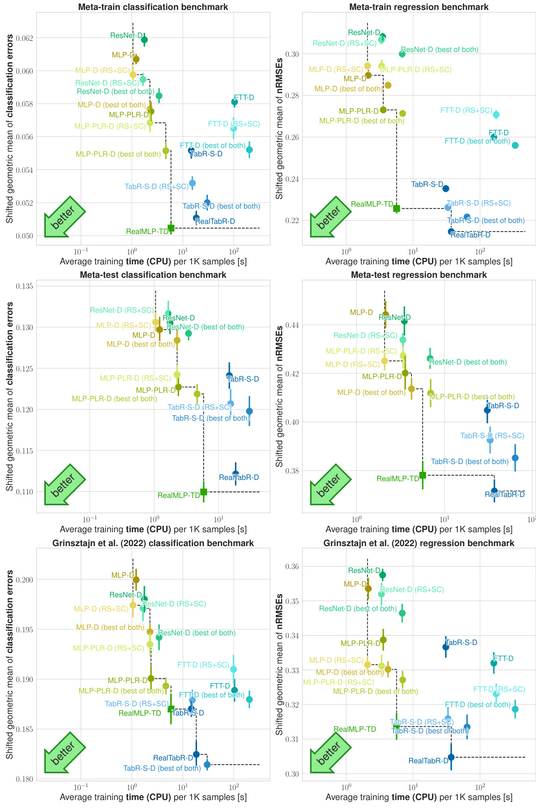
This figure compares various machine learning methods (GBDTs, NNs, ensembles) on four benchmark datasets. The y-axis shows the model’s performance (classification error or nRMSE), while the x-axis displays the training time per 1000 samples. Error bars represent 95% confidence intervals. The plot highlights the trade-off between accuracy and training time for different models and dataset types, showing RealMLP-TD and RealTabR-D to be competitive with GBDTs.

This figure compares the performance of various machine learning models on different benchmarks. The y-axis represents the performance metric (classification error or nRMSE), while the x-axis shows the average training time. The figure shows the trade-off between accuracy and training time for various models with different parameter settings (library defaults, tuned defaults, and hyperparameter optimization). The error bars provide a measure of uncertainty. Overall, this figure visually summarizes the key findings of the paper regarding the comparative performance of different models and parameter tuning methods.

This figure compares multiple machine learning models across various benchmarks, showing the trade-off between their performance (measured by classification error or nRMSE) and training time. The results include models using default parameters, tuned default parameters, and hyperparameter optimization (HPO). Error bars represent the 95% confidence intervals, accounting for variability in the random train-test splits.

This figure compares the performance and training time of various machine learning models on multiple benchmark datasets. The y-axis represents the model’s performance (classification error or nRMSE), using a shifted geometric mean to aggregate results across datasets. The x-axis represents the average training time required per 1000 samples. The models are categorized by the type of model (defaults, tuned defaults, hyperparameter optimization). Error bars indicate 95% confidence intervals.
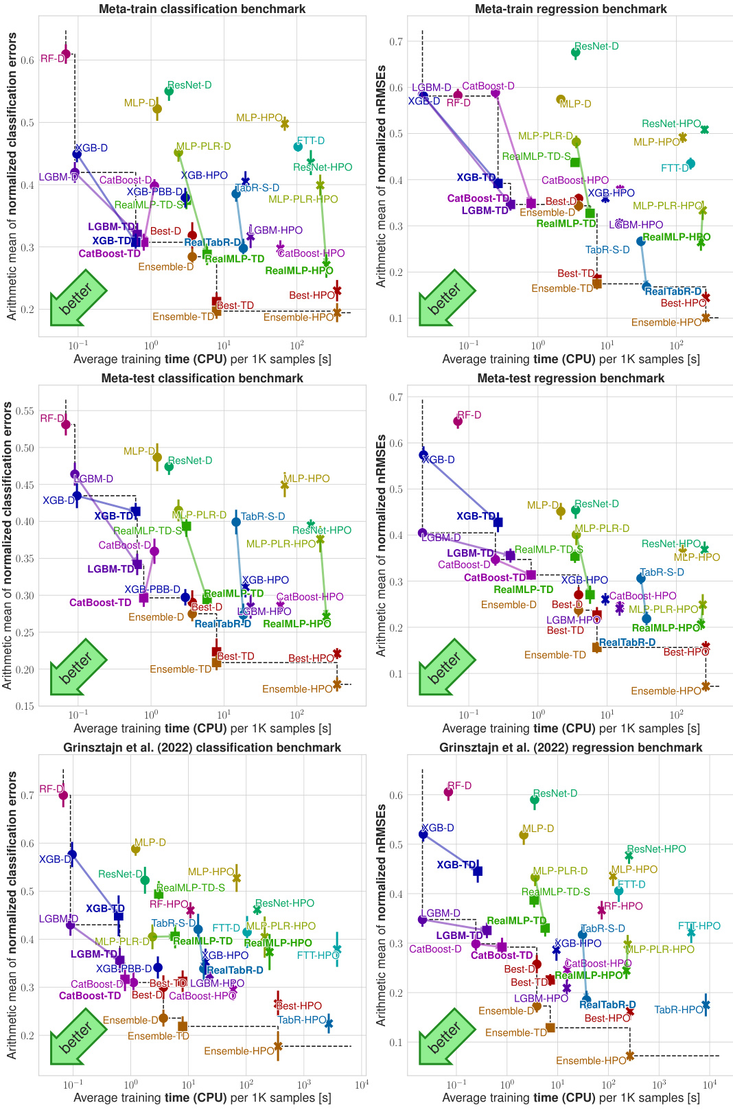
This figure compares the performance of various machine learning models on different benchmark datasets. The y-axis represents the model’s performance (classification error or nRMSE), using a shifted geometric mean to aggregate scores across multiple datasets. The x-axis represents the average training time per 1000 samples. The plot allows for a comparison of the models’ time-accuracy tradeoffs. Error bars depict 95% confidence intervals.
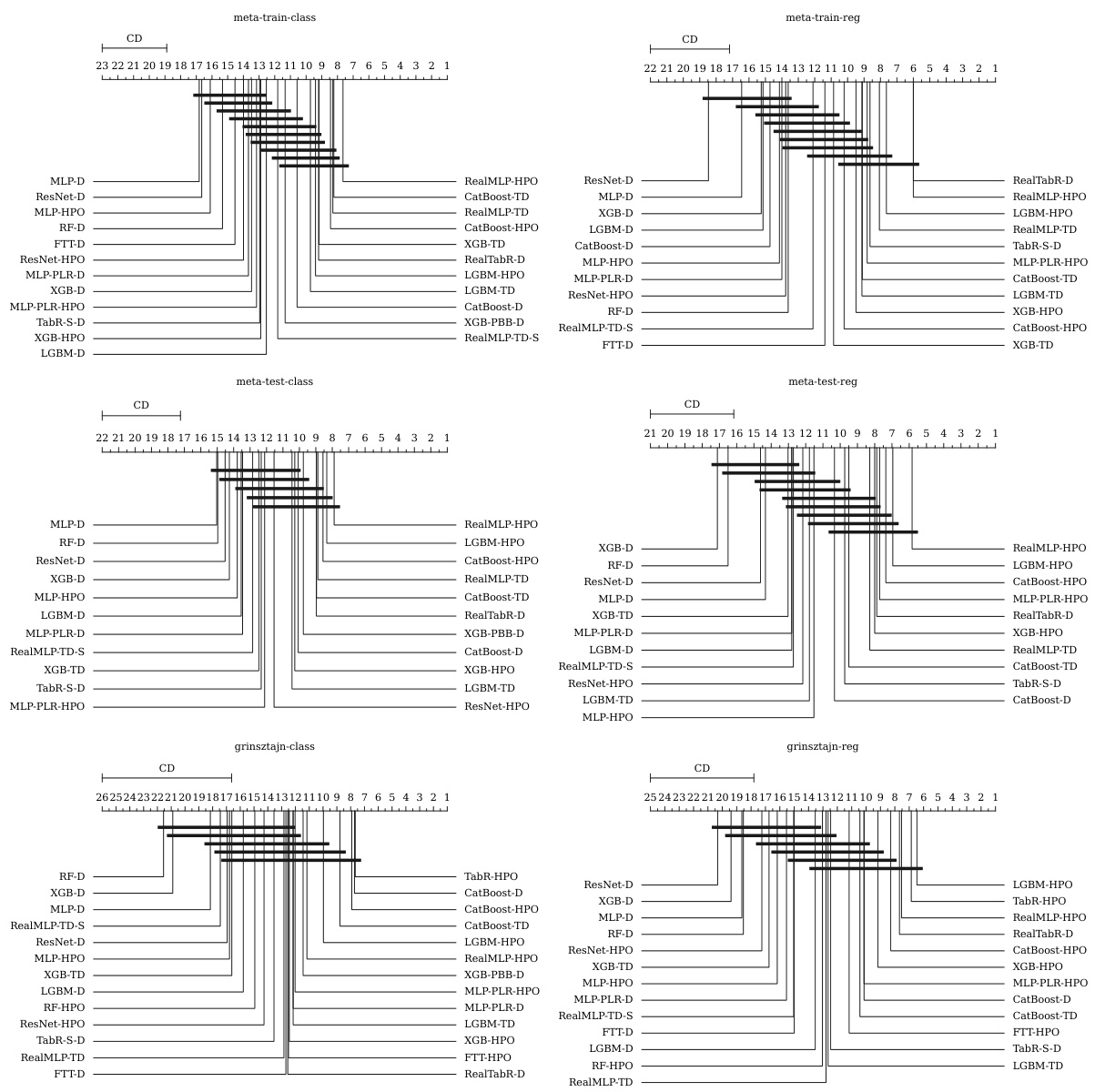
This figure compares the performance of various machine learning models on different benchmark datasets. The y-axis represents the model’s performance (classification error or nRMSE), and the x-axis shows the average training time per 1000 samples. The models are categorized by their type (library defaults, tuned defaults, and hyperparameter optimization). Error bars indicate the 95% confidence intervals, showing the uncertainty in the results. The plot helps visualize the tradeoff between training time and model accuracy across different methods and datasets.
This figure compares different machine learning models on several benchmark datasets. The y-axis shows the performance (error rate for classification, normalized RMSE for regression) of each model, aggregated across multiple runs. The x-axis indicates the training time required by each model. This visualization helps illustrate the speed-accuracy tradeoffs of the different models.

This figure compares different machine learning models’ performance across various benchmarks in terms of accuracy and training time. It shows the shifted geometric mean classification error or normalized root mean squared error (nRMSE) against the average training time per 1000 samples. The models include various gradient boosted decision trees (GBDTs), tuned and untuned versions of a multilayer perceptron (MLP) called RealMLP, and other neural network baselines. Error bars represent 95% confidence intervals for the average training time.

This figure compares various machine learning models on different benchmarks (meta-train classification, meta-train regression, meta-test classification, meta-test regression, Grinsztajn et al. 2022 classification, Grinsztajn et al. 2022 regression). For each benchmark, the y-axis shows the performance (classification error or nRMSE) using a shifted geometric mean. The x-axis shows the average training time per 1000 samples. The models are represented by different colors, and their performance and speed are compared. Error bars show 95% confidence intervals.

This figure compares the performance of various machine learning models on different benchmark datasets. The y-axis represents the model’s performance (classification error or nRMSE), aggregated using a shifted geometric mean. The x-axis shows the average training time required per 1000 samples. Different model types (GBDTs, NNs) and parameter settings (default, tuned defaults, hyperparameter optimization) are compared. The error bars provide a visual representation of the uncertainty in the results.

This figure compares the performance (classification error or nRMSE) and training time of various machine learning models across multiple benchmarks. The y-axis represents the performance metric (lower is better), while the x-axis shows the average training time per 1000 samples. The benchmarks used are: meta-train classification, meta-train regression, meta-test classification, meta-test regression, and the Grinsztajn et al. (2022) benchmarks. Each model is shown in a different color, and error bars representing 95% confidence intervals are provided for better result interpretation. The figure helps visualize the trade-off between model accuracy and training time.

This figure compares various machine learning models’ performance across different benchmarks. The y-axis represents the model’s error (classification error or nRMSE) using a shifted geometric mean to aggregate results from multiple dataset splits. The x-axis shows the average training time per 1000 samples, measured on a meta-training set for efficiency. Error bars represent 95% confidence intervals. The figure facilitates comparison of models based on their time-accuracy trade-off.
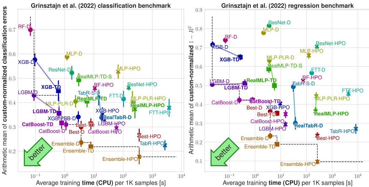
This figure presents a comparison of various machine learning models on different benchmarks, illustrating the tradeoff between accuracy and training time. The y-axis represents the performance (error rate for classification and nRMSE for regression) aggregated across datasets using a shifted geometric mean. The x-axis represents the average training time per 1000 samples. Different model variants (defaults, tuned defaults, hyperparameter-optimized) are compared. The error bars represent 95% confidence intervals, highlighting the statistical significance of the results.
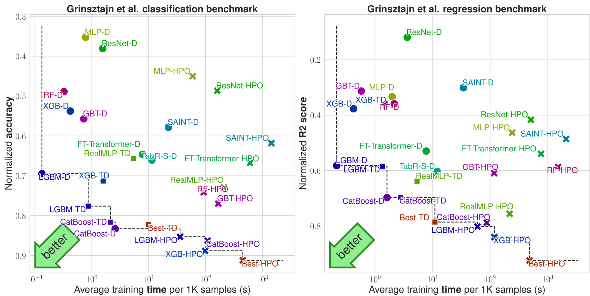
This figure compares multiple machine learning models on their performance across various benchmark datasets in terms of time and accuracy. Specifically, it shows the shifted geometric mean of classification error or normalized root mean squared error (nRMSE) on the y-axis, plotted against average training time per 1000 samples on the x-axis. The models include various gradient-boosted decision trees, as well as different neural network architectures. The figure allows for a direct comparison of the trade-offs between training time and model performance, and also illustrates the effectiveness of using tuned default parameters instead of extensive hyperparameter optimization. Error bars represent the 95% confidence interval.
This figure compares multiple machine learning models’ performance on tabular data classification and regression tasks, considering accuracy and training time efficiency. The y-axis represents the shifted geometric mean of classification errors (left) and normalized root mean squared errors (nRMSE) (right). The x-axis shows the average training time per 1000 samples on the CPU. Different models with varying parameter settings (library defaults, tuned defaults, hyperparameter optimization) are compared, revealing the time-accuracy tradeoffs. Error bars represent 95% confidence intervals.
This figure compares the performance of different machine learning methods across four benchmark datasets in terms of their accuracy and training time. The y-axis represents the average error rate (classification error or normalized root mean squared error), while the x-axis displays the average training time. Each point represents a specific method, with error bars indicating the 95% confidence interval. The figure allows for a visual comparison of the time-accuracy tradeoff of various methods.

This figure compares the performance (in terms of classification error and nRMSE) and training time of various machine learning models across different benchmark datasets. The y-axis represents the performance, calculated using a shifted geometric mean to aggregate results across multiple datasets. The x-axis shows the average training time per 1000 samples. Different model types (GBDTs, MLPs, and other NNs) and parameter tuning strategies (default, tuned defaults, and hyperparameter optimization) are compared. Error bars represent the 95% confidence intervals, indicating the uncertainty in the results.

This figure compares various machine learning models’ performance across different benchmarks in terms of accuracy and training time. The y-axis represents the shifted geometric mean of classification error (for classification tasks) or normalized root mean squared error (nRMSE, for regression tasks). The x-axis represents the average training time per 1000 samples. Each point represents a model’s performance on a benchmark, and the error bars indicate the 95% confidence intervals. This visualization helps to understand the trade-off between accuracy and training time for different models.

This figure compares the performance of various machine learning models on different benchmark datasets. The y-axis shows the performance (classification error or nRMSE), using a shifted geometric mean to aggregate results across datasets. The x-axis represents the average training time for each model. The plot visualizes the time-accuracy trade-off of each model. Error bars indicate 95% confidence intervals.

This figure compares various machine learning models across different benchmarks in terms of their accuracy and training time. The y-axis represents the shifted geometric mean of classification error or normalized root mean squared error (nRMSE), which are aggregate metrics evaluating model performance across multiple datasets. The x-axis shows the average training time for each model on 1000 samples. Error bars represent 95% confidence intervals, providing insights into the uncertainty of the measurements. This visualization helps to understand the trade-off between model accuracy and the time required for training, allowing for comparisons between different model types and hyperparameter settings (defaults, tuned defaults, and hyperparameter optimization).

This figure shows the components of RealMLP-TD, an improved MLP with tuned defaults. It illustrates the architecture, preprocessing steps, and hyperparameter scheduling. Part (c) specifically demonstrates the incremental improvement in benchmark score achieved by adding each component one at a time, with error bars indicating 95% confidence intervals.

This figure compares the performance of various machine learning models across multiple benchmarks. The y-axis represents the model’s error rate (classification error or nRMSE), calculated using a shifted geometric mean to handle potential zero-error cases. The x-axis shows the average training time required per 1000 samples, measured on a subset of the meta-train dataset for computational efficiency. Error bars represent 95% confidence intervals, providing a measure of uncertainty in the results. The figure visually demonstrates the time-accuracy trade-off among different models and across various benchmarks, allowing for a comprehensive comparison of efficiency and performance.
More on tables
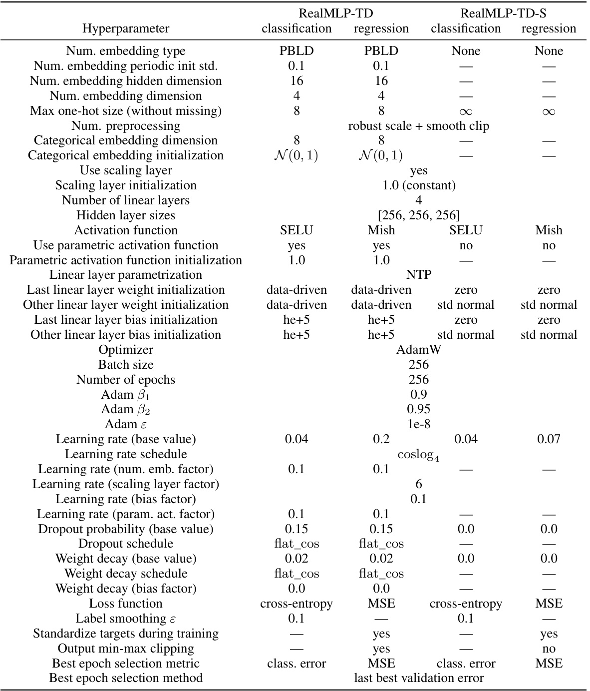
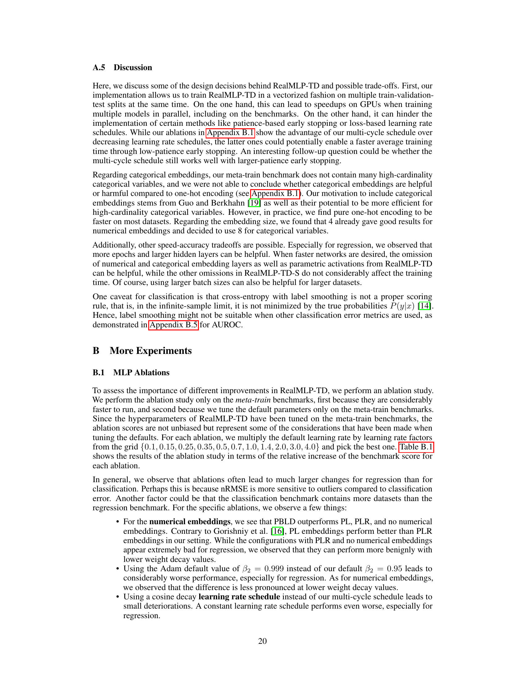
This table provides a detailed overview of the hyperparameters used in the RealMLP-TD and RealMLP-TD-S models. It lists hyperparameters related to numerical and categorical embeddings, preprocessing steps (such as robust scaling and smooth clipping), neural network architecture (number of layers, hidden layer sizes, activation functions), training parameters (optimizer, learning rate, weight decay, etc.), and other hyperparameters. The table also specifies different values used for classification and regression tasks, highlighting the variations in hyperparameter settings depending on the type of task.
This table lists the hyperparameter settings used for the RealMLP-TD and RealMLP-TD-S models. It provides a detailed breakdown of the hyperparameters used in both models, categorized by type (e.g., numerical preprocessing, categorical embedding, NN architecture, initialization, regularization, training, hyperparameters). For each hyperparameter, the table specifies the value used for both classification and regression tasks, as well as noting which hyperparameters are specifically tuned and which ones are kept as library defaults. The table helps clarify the choices made for hyperparameter optimization and the configuration of the different model components.

This table shows the results of comparing different preprocessing methods for numerical features used in the RealMLP-TD-S model. The methods compared include robust scaling with and without smooth clipping, standardization with and without smooth clipping, quantile transformation (with and without the RTDL version used by Gorishniy et al. [15]), and the kernel density integral transformation [42]. The table reports the relative increase in the meta-train classification and regression benchmark scores for each method compared to using robust scaling with smooth clipping. 95% confidence intervals are provided for each result, and the best performing method in each category is highlighted in bold.

This table presents the results of experiments evaluating the impact of bagging and refitting on the performance of LGBM-TD. It compares different configurations: bagging vs. refitting, one model vs. five models, and individual stopping vs. joint stopping. The relative reduction in benchmark scores (shifted geometric mean) are reported, along with 95% confidence intervals. The best scores in each column are highlighted.

This table presents the results of experiments evaluating different strategies to improve the performance of LGBM-TD, a gradient boosting decision tree model. The strategies tested involve bagging (training multiple models on different subsets of the data), refitting (training a single model on the full dataset multiple times), using 1 or 5 models, and performing individual stopping or joint stopping (choosing the best epoch/iteration based on individual models or the ensemble). The table shows the improvement in performance (reduction in shifted geometric mean error) for each strategy, along with 95% confidence intervals. The best-performing configurations are highlighted.

This table presents a detailed breakdown of the hyperparameter settings used for both RealMLP-TD and its simplified version, RealMLP-TD-S. It covers various aspects of the models, including data preprocessing techniques, neural network architecture details (such as the number of layers, neuron counts, activation functions, and embedding methods), optimization parameters (like learning rate, weight decay, optimizer, and scheduling), and training specifics (batch size, number of epochs, and stop criteria). The table distinguishes between settings for classification and regression tasks, highlighting any differences in hyperparameter choices for these two scenarios. This level of detail is crucial for understanding how RealMLP-TD was designed and trained, and provides the necessary information for others to reproduce the experiments.

This table presents the hyperparameters used for LightGBM in two settings: TD (tuned defaults) and D (library defaults). It shows the values of parameters such as
num_leaves,learning_rate,subsample,colsample_bytree,min_data_in_leaf,min_sum_hessian_in_leaf,n_estimators,bagging_freq,max_bin, andearly_stopping_rounds. The values for the TD setting were tuned using the meta-training benchmark, while the D setting uses the default values provided by the LightGBM library. Italicized hyperparameters indicate those which were not tuned in the TD setting.

This table presents the hyperparameter settings for the XGBoost model, comparing the tuned defaults (TD) with the library defaults (D). It shows hyperparameters for both classification and regression tasks. Note that some hyperparameters were not tuned for the XGB-TD model. The table is part of the Benchmark Details section within the paper.
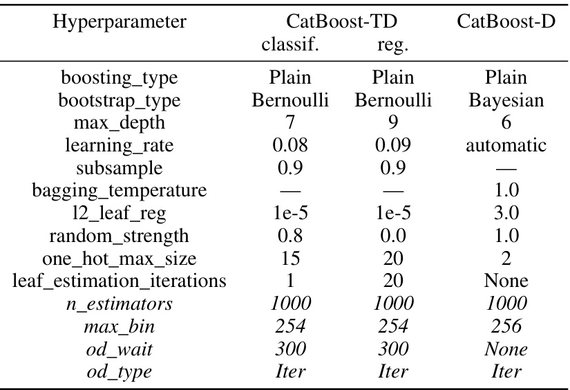
This table lists the hyperparameters used for CatBoost in two scenarios: tuned defaults (TD) and library defaults (D). The table is divided into sections for classification and regression tasks, showing the specific hyperparameter values used in each scenario. Italicized hyperparameters indicate those that were not tuned for the TD setting, suggesting the library defaults were retained for those parameters in the tuned default configuration. The table provides a detailed comparison of the hyperparameter settings used for CatBoost in both the tuned default and library default scenarios.

This table provides a detailed list of hyperparameters used in the RealMLP-TD and RealMLP-TD-S models. It breaks down the hyperparameters into categories such as those related to numerical and categorical feature embedding, preprocessing steps (robust scaling and smooth clipping), neural network architecture (number of layers, activation functions), training settings (optimizer, learning rate schedule), and regularization techniques (dropout, weight decay). The table also shows differences in hyperparameter settings between RealMLP-TD and its simplified version, RealMLP-TD-S. This level of detail allows for a better understanding of how the models are configured and aids in reproducibility.

This table lists the hyperparameters used for the RealMLP-TD and RealMLP-TD-S models. It details the settings for various aspects of the models, including data preprocessing, the neural network architecture (embedding types, number of layers, activation functions, etc.), optimization parameters (optimizer, learning rate, weight decay, etc.), and training parameters (batch size, number of epochs, etc.). The table distinguishes between settings used for classification tasks and those used for regression tasks. It shows the specific values used in the default (TD) parameter setting for both models.
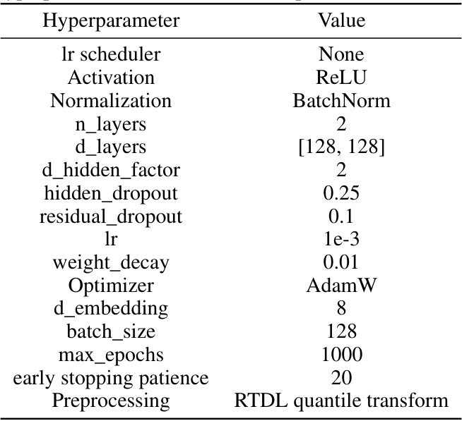
This table presents a detailed overview of the hyperparameter settings used for both RealMLP-TD and its simplified version, RealMLP-TD-S. It covers various aspects of the models, including data preprocessing techniques (such as robust scaling and smooth clipping, one-hot encoding, and numerical embeddings), neural network architecture (number of layers, hidden layer sizes, activation functions, dropout, scaling layers, periodic bias linear dense net embeddings), training parameters (optimizer, learning rate schedules, weight decay), and other hyperparameters. The table helps to understand the differences and similarities between the two models, providing a comprehensive view of the hyperparameter choices made during model development.
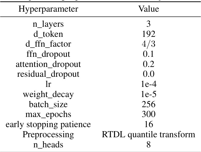
This table provides a comprehensive overview of the hyperparameters used in the RealMLP-TD and RealMLP-TD-S models. It meticulously lists each hyperparameter, specifying its value for both classification and regression tasks. The table is organized to clearly show the differences in hyperparameter settings between the two models (RealMLP-TD and RealMLP-TD-S), highlighting choices made for specific components like numerical and categorical embeddings, activation functions, and optimization strategies. This level of detail aids in understanding the design choices and their impact on model performance.
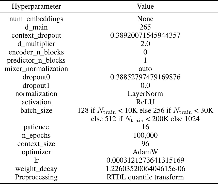
This table provides a detailed overview of the hyperparameters used in the RealMLP-TD and RealMLP-TD-S models. It breaks down the hyperparameters into categories such as those related to numerical and categorical embeddings, preprocessing steps, activation functions, optimization parameters, and training settings. The table shows specific values used for both classification and regression tasks, highlighting any differences in hyperparameter settings between the two model versions and the two tasks. The level of detail provided allows for a comprehensive understanding of the configuration choices made for these models.
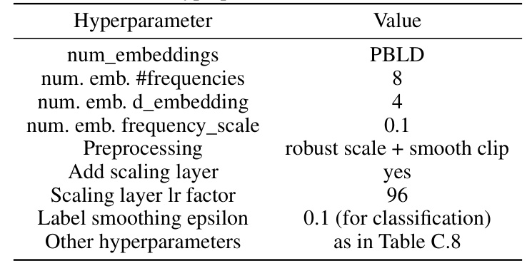
This table presents the hyperparameters used for the RealTabR-D model. It includes settings for numerical embeddings (PBLD type), the number of frequencies and embedding dimensions, frequency scale, preprocessing steps (robust scaling and smooth clipping), the use of a scaling layer and its learning rate factor, and label smoothing epsilon. Other hyperparameters are the same as those used in the TabR-S-D model (as referenced in Table C.8).
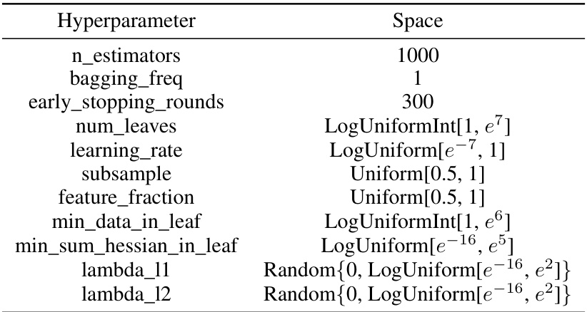
This table shows the hyperparameter search space used for hyperparameter optimization of LightGBM. The search space includes parameters such as the number of estimators, bagging frequency, early stopping rounds, number of leaves, learning rate, subsample ratio, feature fraction, minimum data in leaf, and regularization parameters (lambda_l1 and lambda_l2). The values are specified using different distributions like LogUniformInt, LogUniform, and Uniform, which represent the distributions used when sampling the hyperparameters. The search space is adapted from Prokhorenkova et al. [51], with 1000 estimators instead of the original 5000, to balance efficiency and accuracy in the meta-learning context of the study.
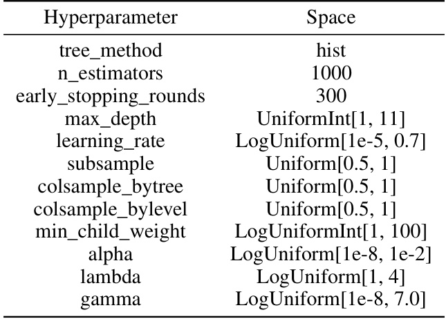
This table presents the hyperparameter search space used for hyperparameter optimization (HPO) of the XGBoost model. It specifies the ranges and distributions for each hyperparameter, including the tree method, number of estimators, early stopping rounds, max depth, learning rate, subsample, colsample_bytree, colsample_bylevel, min_child_weight, alpha, lambda, and gamma. The choices made reflect updates to XGBoost since the original paper by Grinsztajn et al. [18] was published.
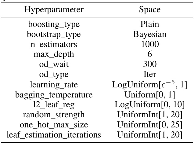
This table presents the hyperparameter search space used for hyperparameter optimization (HPO) of the Light Gradient Boosting Machine (LGBM) model. The search space defines the range and distribution of values for each hyperparameter, which are used during the random search process to find the optimal hyperparameter configuration for the LGBM model. The hyperparameters include: number of estimators, bagging frequency, early stopping rounds, number of leaves, learning rate, subsample ratio, feature fraction, minimum data in leaf, minimum sum of hessian in leaf, L1 regularization, and L2 regularization.

This table presents the hyperparameter search space used for random forest (RF) hyperparameter optimization (HPO) in the Grinsztajn et al. [18] benchmark. The search space defines the range of values considered for each hyperparameter during the optimization process. These hyperparameters include the number of trees, maximum tree depth, splitting criterion, number of features considered at each split, minimum samples required for a split, minimum samples required for a leaf node, whether bootstrapping is used, and minimum decrease in impurity required for a split. The probability distributions for some of the hyperparameters are also specified.

This table provides a detailed overview of the hyperparameters used in the RealMLP-TD and RealMLP-TD-S models. It breaks down hyperparameters into categories such as data preprocessing, network architecture, optimization, initialization, and regularization. For each hyperparameter, the table specifies the value used in RealMLP-TD and RealMLP-TD-S for both classification and regression tasks, highlighting differences in parameter settings between the two model variations and between classification and regression.

This table presents the hyperparameter search space used for optimizing the LightGBM model. It lists various hyperparameters, their data types (such as integers or floating-point numbers), and the range of values considered during the search. The search space aims to find optimal hyperparameter settings for the LightGBM model that improve its performance on tabular data.

This table presents the hyperparameter search space used for hyperparameter optimization of the MLP-PLR model. It is adapted from Gorishniy et al. [16], but with modifications to the search space for σ (following private communication with an author), and the maximum embedding dimension (reduced to 64 to manage memory usage). The MLP portion of the search space is the same as that used for MLP-HPO in Table C.15.
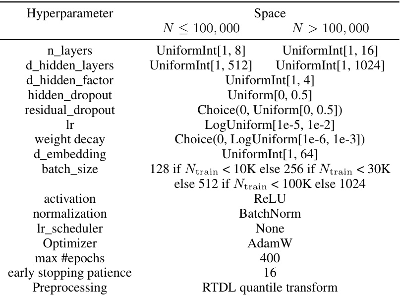
This table shows the hyperparameter search space used for hyperparameter optimization of LightGBM model in the paper. It specifies ranges or choices for various hyperparameters, including the number of estimators, learning rate, subsample ratio, feature fraction, minimum data in leaf, minimum sum hessian in leaf, lambda_l1 and lambda_l2. The values provided are ranges or distributions from which the hyperparameter optimizer randomly samples during the search process. The search space is adapted from Prokhorenkova et al. [51], but the number of estimators is reduced from 5000 to 1000 to balance efficiency and accuracy.

This table presents the hyperparameter search space used for the FT-Transformer model in the hyperparameter optimization (HPO) experiments. It shows the ranges and choices for each hyperparameter, including the number of layers, token dimension, feed-forward network dimension factor, dropout rates, learning rate, weight decay, batch size, number of epochs, early stopping patience, preprocessing method (RTDL quantile transform), and number of attention heads. The modifications from the original paper are noted.

This table presents the hyperparameter search space used for hyperparameter optimization (HPO) of the TabR model. It shows the range of values considered for each hyperparameter during the HPO process. Some hyperparameters, not specified in the original paper by Gorishniy et al., were chosen based on TabR-S-D settings (Table C.8). Notably, the weight decay hyperparameter’s upper bound differs from the original paper.
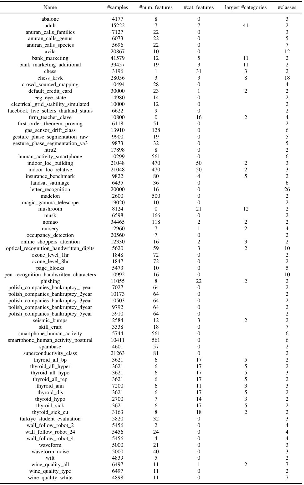
This table lists the characteristics of the datasets used in the meta-train classification benchmark. For each dataset, it shows the number of samples, the number of numerical features, the number of categorical features, the largest number of categories in any categorical feature, and the number of classes. This information is crucial for understanding the composition of the benchmark used for tuning the default hyperparameters.

This table lists the characteristics of datasets used in the meta-train classification benchmark. For each dataset, it shows the dataset name, number of samples, number of numerical features, number of categorical features, the largest number of categories in any categorical feature, and the number of classes. This information is used to evaluate the performance of various machine learning models.

This table lists the characteristics of the datasets used in the meta-train classification benchmark. For each dataset, it provides the name, number of samples, number of numerical features, number of categorical features, the largest number of categories in any categorical feature, and the number of classes.
This table presents the hyperparameters used for the Light Gradient Boosting Machine (LGBM) model. It shows two sets of hyperparameters, one for LGBM with tuned default parameters (LGBM-TD) and one for LGBM with the default parameters from the library (LGBM-D). For each set, it specifies the hyperparameters for both classification and regression tasks. The table helps to understand the differences in hyperparameter settings between the tuned and default versions of the LGBM model. The italicized hyperparameters are those that were not tuned.

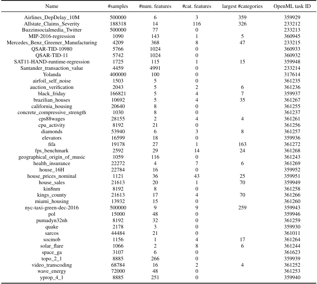
This table provides a detailed list of datasets used in the meta-test classification benchmark. For each dataset, it shows the number of samples, the number of numerical features, the number of categorical features, the largest number of categories in any categorical feature, the number of classes in the target variable, and the corresponding OpenML task ID. This information is crucial for understanding the characteristics of the data used in evaluating the models and for reproducibility.
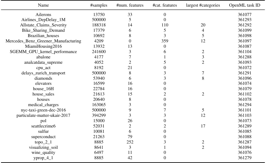
This table provides a list of datasets used in the meta-test classification benchmark. For each dataset, it shows the number of samples, number of numerical features, number of categorical features, the largest number of categories in a categorical feature, the number of classes, and the OpenML task ID. The table gives an overview of the characteristics of the datasets used in the meta-test classification benchmark, which is a subset of the larger meta-test benchmark that includes both classification and regression tasks.
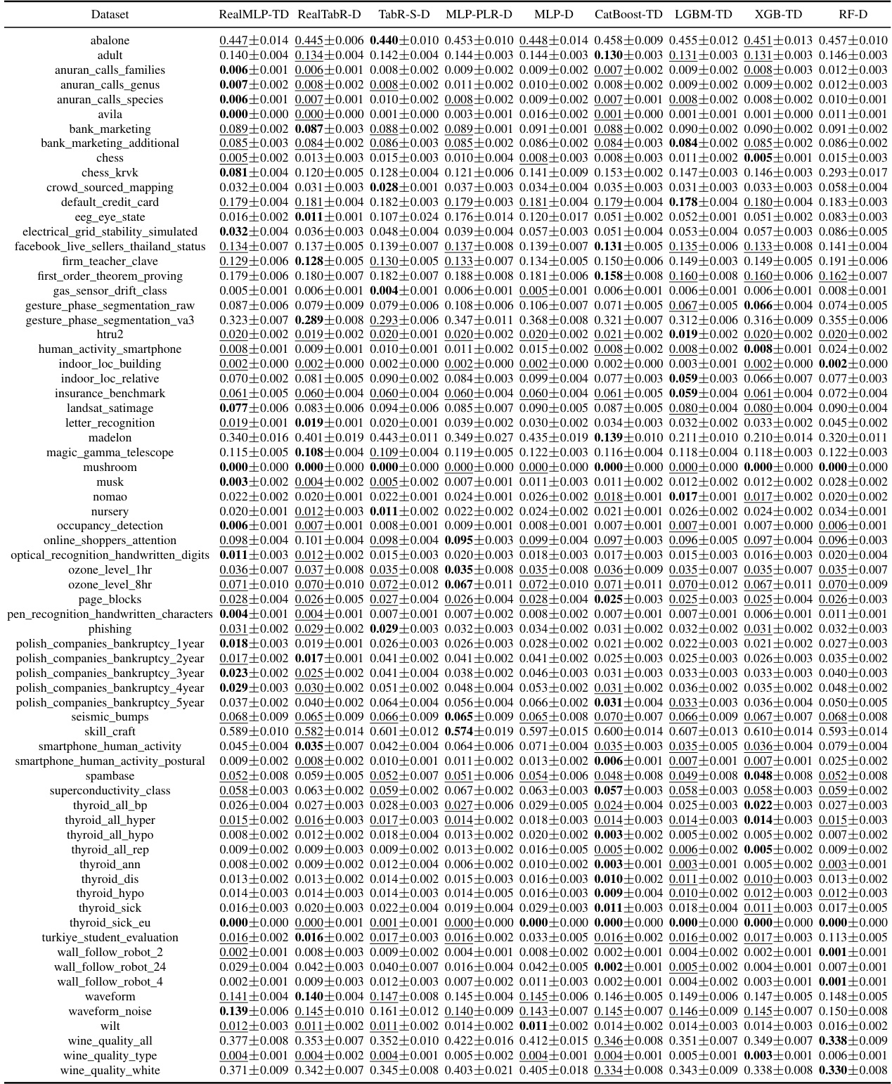
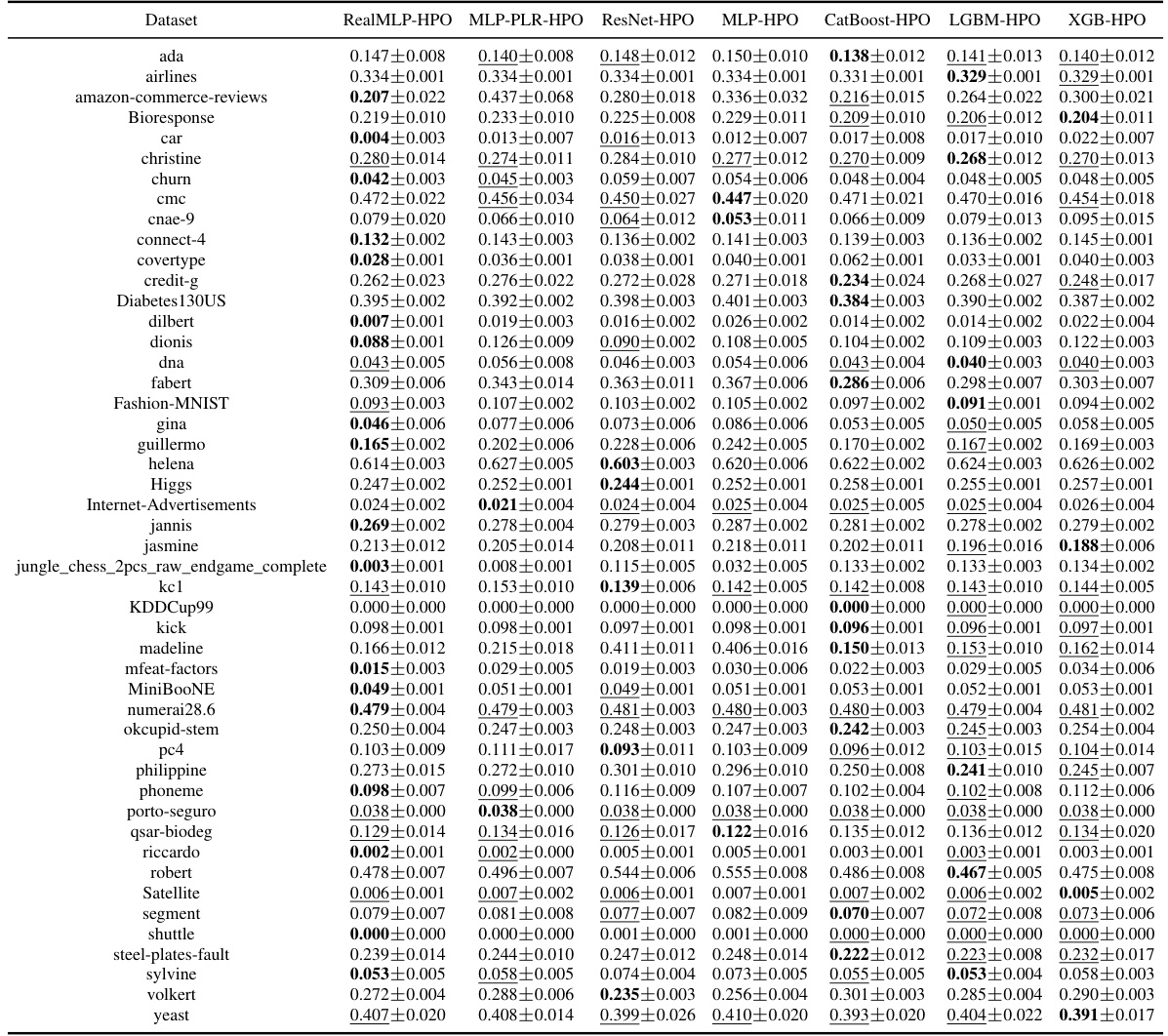
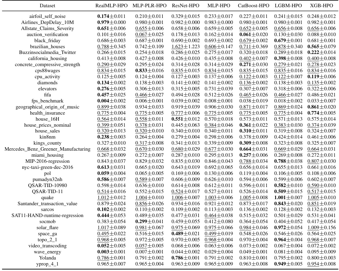
This table presents the classification error of eight different machine learning methods on 71 datasets in the meta-train classification benchmark. For each dataset, the table shows the mean classification error and a 95% confidence interval. The lowest mean classification error for each dataset is highlighted in bold, and any errors whose confidence intervals overlap the lowest are also underlined.
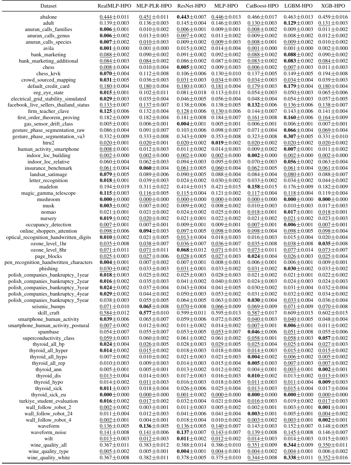
This table presents the classification error rates of various untuned machine learning models on a set of datasets. The table shows the mean error and a 95% confidence interval for each model and dataset, highlighting the model with the lowest average error rate for each dataset.

This table presents the classification error for multiple untuned machine learning models across various datasets from the meta-train benchmark. The results are averages over ten train-validation-test splits, and the table also shows approximate 95% confidence intervals calculated using a t-distribution. The lowest mean error in each row is highlighted, and errors whose confidence intervals include the lowest mean error are also marked.

This table presents the hyperparameter search space used for hyperparameter optimization (HPO) of the Light Gradient Boosting Machine (LGBM) model. The search space defines the ranges and distributions for various hyperparameters, such as the number of leaves, learning rate, subsample ratio, feature fraction, minimum data in leaf, minimum sum of hessian in leaf, L1 regularization, and L2 regularization. The values are chosen to balance exploration of the hyperparameter space with computational efficiency during HPO. The original number of estimators was 5000, but it has been reduced to 1000 in this study.

This table presents the classification error of several untuned machine learning models on the meta-train dataset. The error is calculated as an average over ten train-validation-test splits and includes an approximate 95% confidence interval. The lowest mean error for each dataset is bolded and errors whose confidence intervals include the lowest error are underlined. The table is designed to compare the performance of various models across different datasets.
This table lists the hyperparameters used for LightGBM (LGBM) in two different settings: LGBM-TD (tuned default parameters) and LGBM-D (library default parameters). The table shows the values for each hyperparameter, differentiating between classification and regression tasks. Italicized hyperparameters indicate those that were not tuned for LGBM-TD. This is essential for understanding how the default parameters were modified to achieve improved performance in the LGBM-TD setting, as described in the paper.
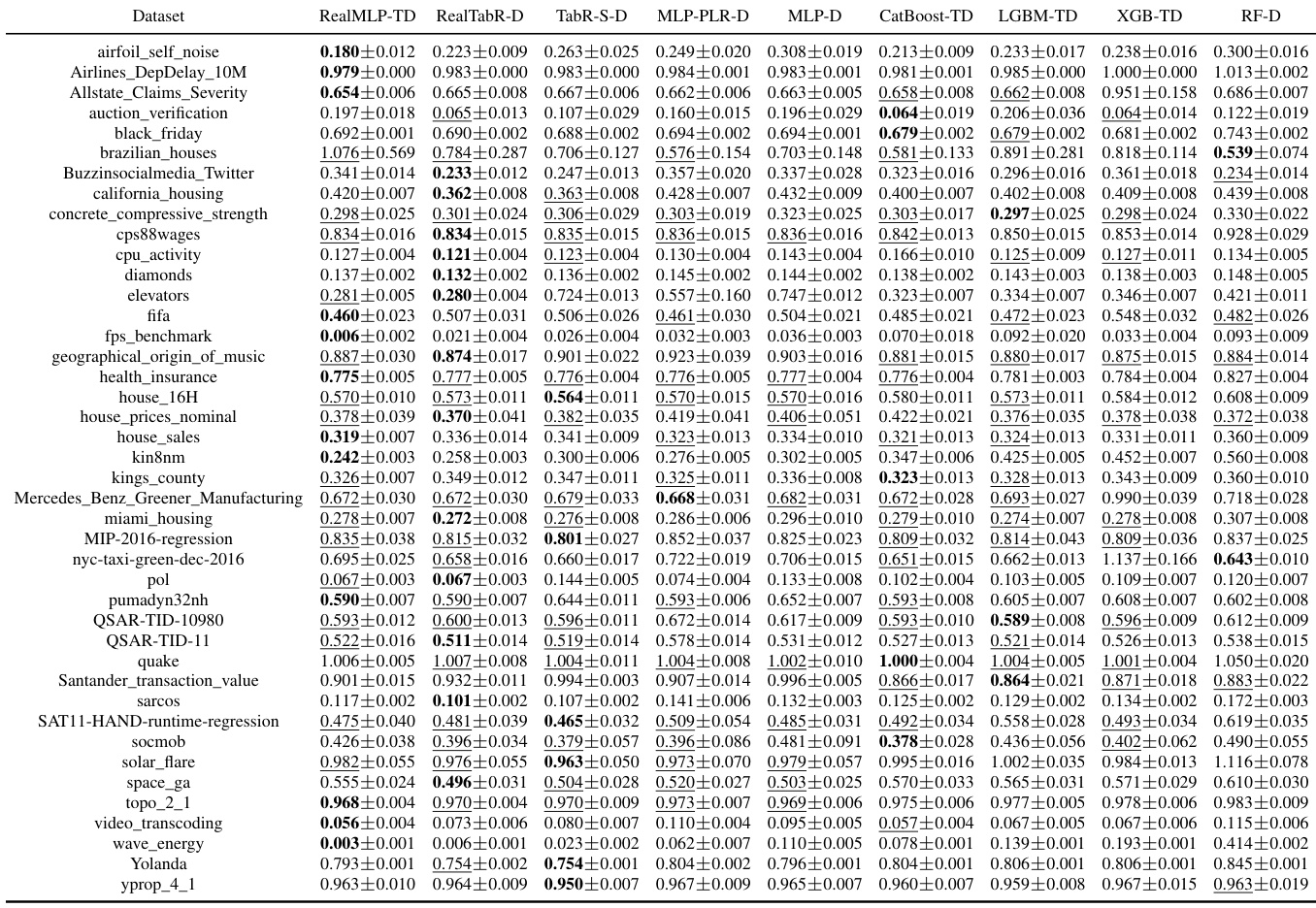
This table shows the classification error rates of various untuned machine learning models on a set of datasets from the meta-train benchmark (Btrain). The results are averages over ten train/validation/test splits, and error bars show approximate 95% confidence intervals calculated using a t-distribution. The lowest mean error in each row is bolded, and rows where the confidence interval overlaps the lowest error are underlined. The models compared include RealMLP-TD, RealTabR-D, TabR-S-D, MLP-PLR-D, MLP-D, CatBoost-TD, LGBM-TD, XGB-TD, and RF-D.
This table presents the hyperparameter search space used for hyperparameter optimization (HPO) of LightGBM. The search space defines the range and distribution of values considered for each hyperparameter during the HPO process. The number of estimators is fixed at 1000, unlike in the original paper by Prokhorenkova et al. [51].

This table presents the classification error rates of several machine learning models on various datasets from the meta-train classification benchmark. The error rates are averages across ten different train/validation/test splits of each dataset. The table also provides approximate 95% confidence intervals for the average error rates, calculated using the t-distribution and a normality assumption. The lowest average error rate for each dataset is highlighted in bold, and those within one standard error of the lowest are underlined.

This table presents the hyperparameter search space used for hyperparameter optimization (HPO) of the LightGBM model. It lists the hyperparameters, their type, and the range of values explored during the random search process. The search space is adapted from Prokhorenkova et al. [51], but with 1000 estimators instead of 5000, reflecting a balance between efficiency and accuracy.

This table shows the nRMSE (normalized Root Mean Squared Error) of several untuned machine learning methods on the Grinsztajn et al. [18] classification benchmark. For each dataset, the table presents the mean nRMSE and an approximate 95% confidence interval, calculated using the t-distribution. The lowest mean nRMSE for each dataset is bolded, and any other nRMSE values whose confidence intervals overlap with the lowest are also underlined.

This table presents the classification error rates for various tuned machine learning methods on the Grinsztajn et al. [18] classification benchmark. For each dataset, the average error and a 95% confidence interval are shown. The best-performing method for each dataset is highlighted.
Full paper#
