↗ OpenReview ↗ NeurIPS Homepage ↗ Chat
TL;DR#
The Bahncard problem, a generalization of the ski-rental problem, challenges online algorithms to make irrevocable, repeated decisions between cheap short-term and expensive long-term solutions with unknown future demands. Existing algorithms like SUM struggle to handle prediction errors effectively. Previous attempts such as SUMw and FSUM had limitations in consistency and robustness.
This paper introduces PFSUM, a novel learning-augmented algorithm designed to overcome these limitations. PFSUM cleverly integrates both past performance and predicted future costs to make more informed online decisions. The researchers rigorously prove PFSUM’s competitive ratio, showing it’s both consistent (performs well with perfect predictions) and robust (handles prediction errors gracefully). Extensive experiments demonstrate that PFSUM significantly outperforms existing algorithms, making it a valuable contribution to the field.
Key Takeaways#
Why does it matter?#
This paper is crucial for researchers working on online algorithms with predictions, particularly those dealing with problems involving repeated decisions between short-term and long-term solutions. It offers a novel algorithm, PFSUM, that significantly outperforms existing methods and provides a strong theoretical framework for analysis, pushing forward the field of learning-augmented algorithms and setting a new benchmark for performance and robustness.
Visual Insights#

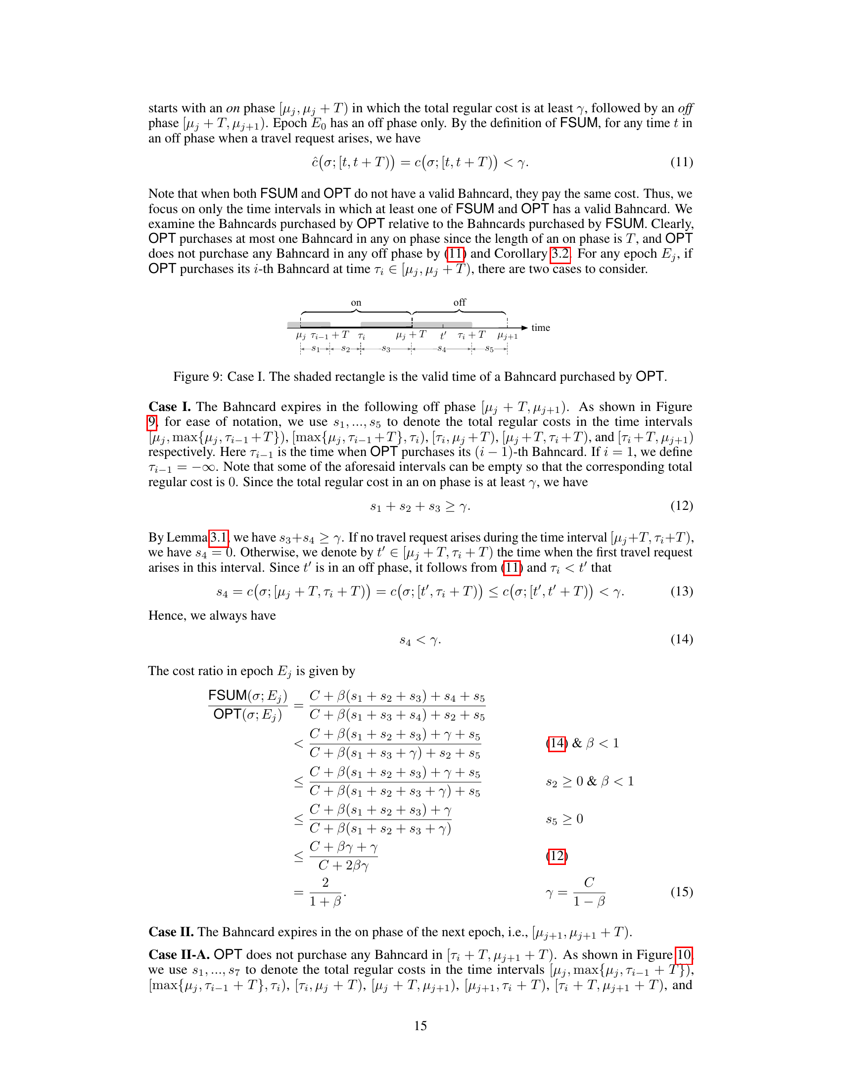
This figure illustrates Lemma 4.4, which states that if a time interval [t, t+T) overlaps with an off phase, and the costs in the preceding on phase (s2), off phase (s3), and succeeding on phase (s4) are less than or equal to γ and γ, respectively, then the total cost in [t,t+T) is at most 2γ+η. The shaded rectangle represents the time period when OPT (optimal offline algorithm) has a valid Bahncard. The figure visually depicts the different cost components (s2, s3, s4) and their relationship to the Lemma.
In-depth insights#
Bahncard Algorithmic Study#
A Bahncard Algorithmic Study would delve into the optimization challenges presented by the German Bahncard railway pass. The core problem involves strategically deciding between purchasing a Bahncard (long-term, potentially cheaper with discounts) versus buying individual tickets (short-term, simpler). The algorithm’s design must account for the unpredictable nature of future travel needs, which makes online decision-making crucial. A comprehensive study would explore different algorithmic approaches, such as primal-dual methods, and evaluate their performance using metrics like competitive ratio, considering various scenarios like different ticket prices, Bahncard validity periods, and prediction accuracy of future travel demand. Machine learning integration could be a key area, leveraging predictive models to improve decision-making. The study should also analyze the trade-offs between algorithm complexity and performance, potentially comparing deterministic and randomized algorithms, and discussing the practical implications and limitations of each approach. A key element is quantifying the robustness of algorithms to prediction errors and exploring strategies for handling uncertain future travel plans.
PFSUM Algorithm#
The PFSUM algorithm, a learning-augmented approach for the Bahncard problem, represents a significant advancement in online decision-making. It cleverly integrates both historical data (past costs) and short-term predictions of future costs, overcoming limitations of previous methods that relied solely on past information or complete future predictions. This dual consideration allows PFSUM to achieve a superior balance between consistency and robustness. The algorithm’s competitive ratio is demonstrably better than previous methods, particularly when prediction errors are present, showing its ability to adapt to imperfect information. This algorithm highlights the power of integrating machine learning insights into traditional online algorithms, improving their performance in realistic scenarios where perfect prediction is not achievable. The 2/(1+β) consistency and 1/β robustness metrics demonstrate its efficiency under various conditions, showcasing PFSUM as a robust and effective solution for online cost minimization problems with uncertain future information.
Prediction Error Impact#
Analyzing a research paper’s section on ‘Prediction Error Impact’ requires a nuanced understanding of how prediction errors affect the performance of algorithms. The key is to examine how the algorithm handles uncertainty. Does it gracefully degrade with increasing error, maintaining a reasonable competitive ratio? Or does performance sharply decline, rendering it impractical for real-world applications with imperfect predictions? A thorough analysis would delve into the algorithm’s design, specifically looking at how it incorporates predictions into its decision-making process. Mathematical analysis of the competitive ratio as a function of prediction error is crucial, showing whether the algorithm remains robust even with significant errors. Empirical evaluation is also key. The experiments should assess the algorithm’s performance under various levels of prediction error, comparing its behavior to alternative approaches or optimal solutions. Visualizations like plots showing the cost ratio or other performance metrics versus prediction error are essential, giving a clear understanding of the impact. Finally, the discussion should carefully assess the practical significance of the findings. What level of prediction accuracy is required for acceptable performance? How do these results relate to real-world applications where perfect predictions are rarely achievable? The ultimate aim is to ascertain the algorithm’s reliability and applicability in situations where prediction errors are unavoidable.
Experimental Setup#
A robust experimental setup is crucial for validating the claims of a research paper. In the context of this research paper, a strong experimental setup would involve a detailed description of the data generation process, including the distributions and parameters used to simulate the Bahncard problem. It should also cover the methods employed to evaluate algorithm performance and the evaluation metrics used, such as the competitive ratio and average cost ratio. Clearly articulating the number of experimental runs, the use of confidence intervals, and the handling of prediction errors is essential for ensuring reproducibility and reliability. The setup needs to consider various aspects such as ticket price distributions (uniform, normal, Pareto), traveler profiles (commuters, occasional travelers), different prediction error levels, and the parameters of the proposed algorithm. Moreover, the setup must clearly define how it will incorporate the short-term predictions and the prediction error levels used in different algorithms. A well-designed setup will carefully address any potential biases that might affect the results, such as the choice of prediction models or the characteristics of the generated data. The selection of both baseline algorithms and parameter ranges needs to be justified to eliminate any potential for confirmation bias. Finally, a strong setup will provide enough information that readers can independently replicate the experiment and verify the findings.
Future Research#
Future research directions stemming from this Bahncard problem study could explore several promising avenues. Extending the algorithm to handle more complex scenarios, such as varying Bahncard validity periods, dynamic pricing, or multiple Bahncard options, would enhance practical applicability. Investigating alternative prediction models beyond the short-term predictions used here, perhaps incorporating long-term trends or incorporating contextual information (travel patterns, seasonality), could lead to improved algorithm performance. A rigorous theoretical analysis of the algorithm’s robustness and consistency under various prediction error distributions would provide stronger theoretical guarantees. Empirical evaluation on real-world datasets is crucial to validate the algorithm’s effectiveness and generalizability. Finally, exploring the application of similar learning-augmented approaches to other online decision-making problems exhibiting renting-or-buying dynamics would broaden the impact of this research.
More visual insights#
More on figures
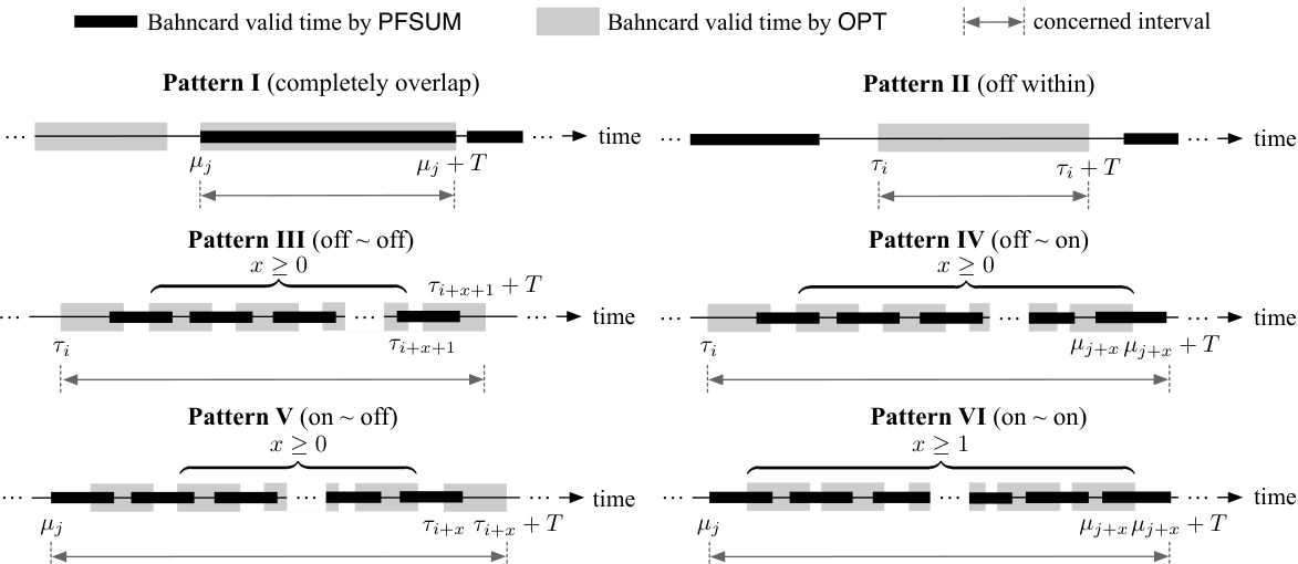
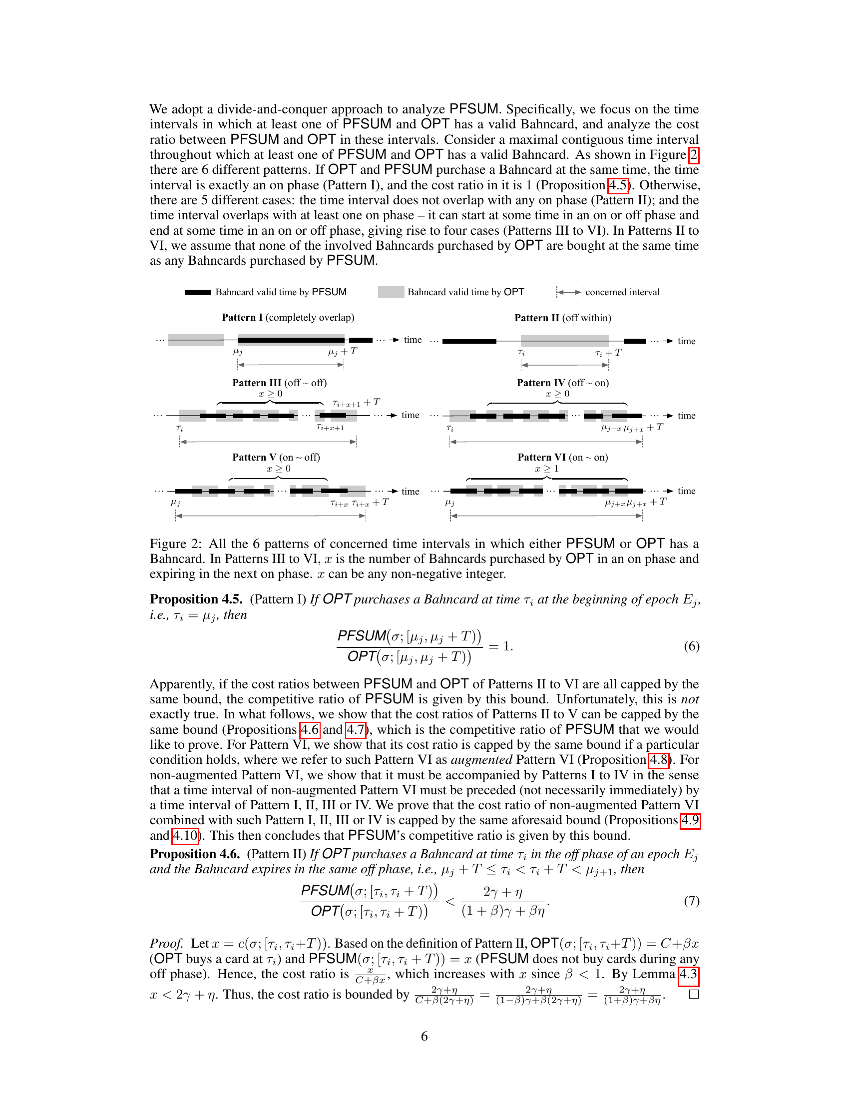
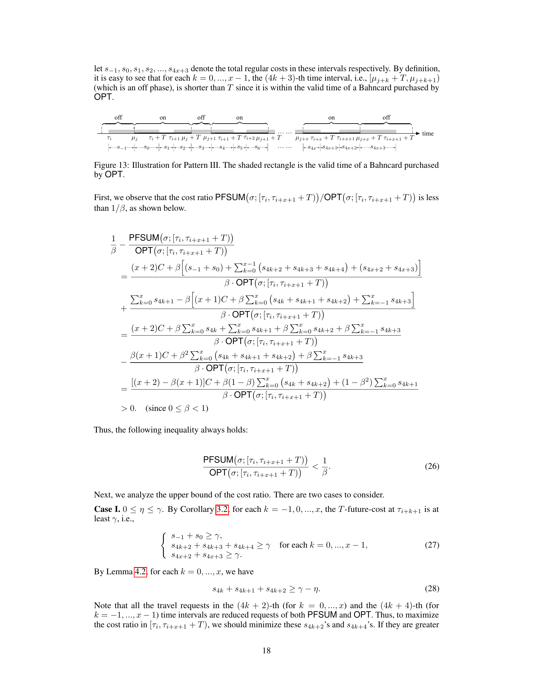
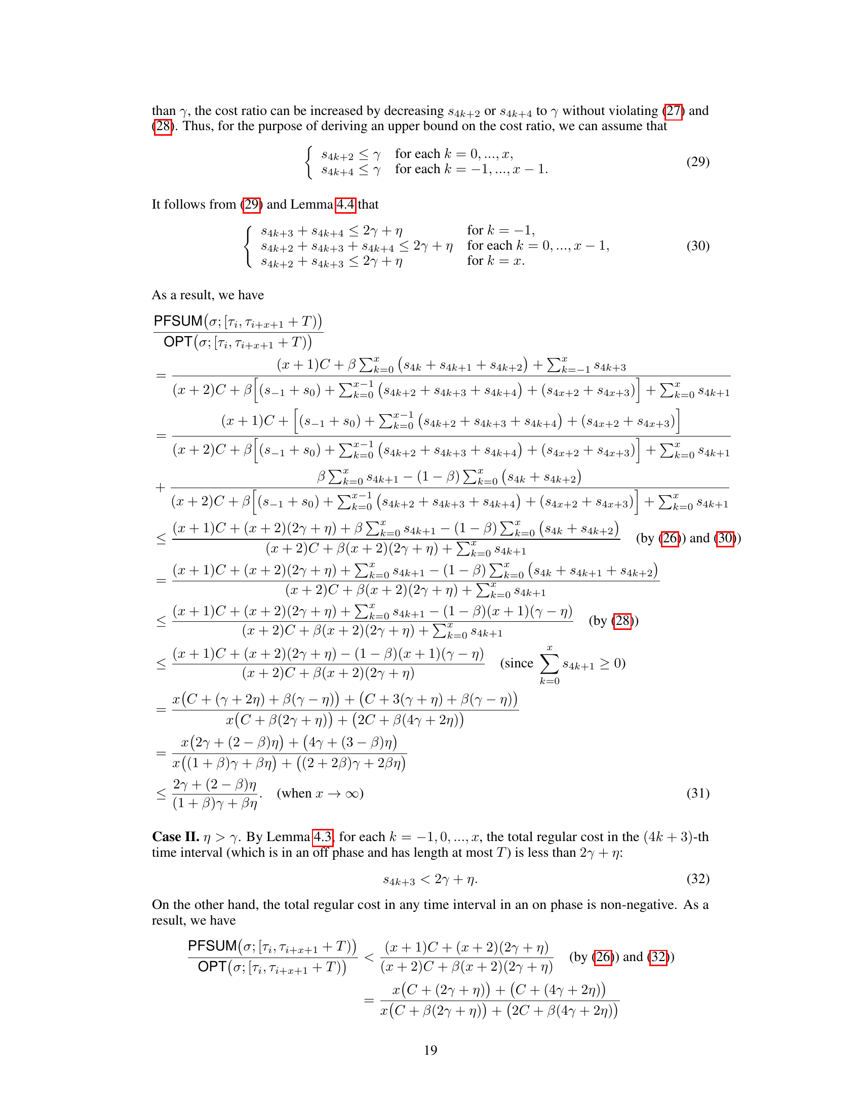
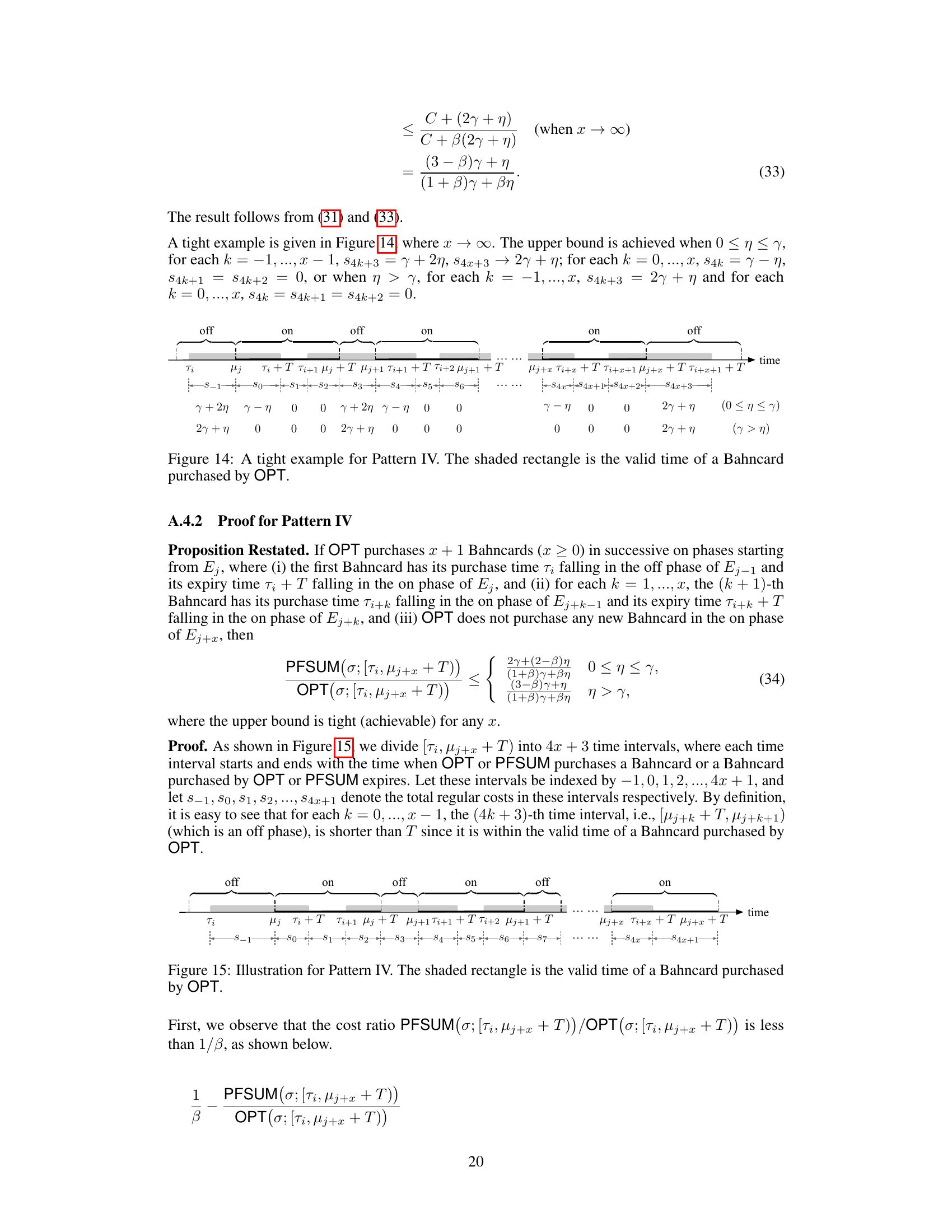
This figure shows six different patterns of time intervals where at least one of the two algorithms (PFSUM and OPT) has a valid Bahncard. The patterns illustrate the various ways the Bahncard validity periods of PFSUM and OPT can overlap. The ‘x’ variable represents the number of Bahncards purchased by OPT within a specific pattern, highlighting the potential variations in Bahncard usage strategies between the two algorithms.

This figure illustrates six patterns of time intervals where at least one of the two algorithms (PFSUM and OPT) has a valid Bahncard. Patterns I through VI represent various overlapping scenarios of Bahncard validity between PFSUM and OPT, with ‘x’ denoting the number of Bahncards purchased by OPT within a specific time frame. This is crucial for the divide-and-conquer analysis in the paper to determine the competitive ratio.

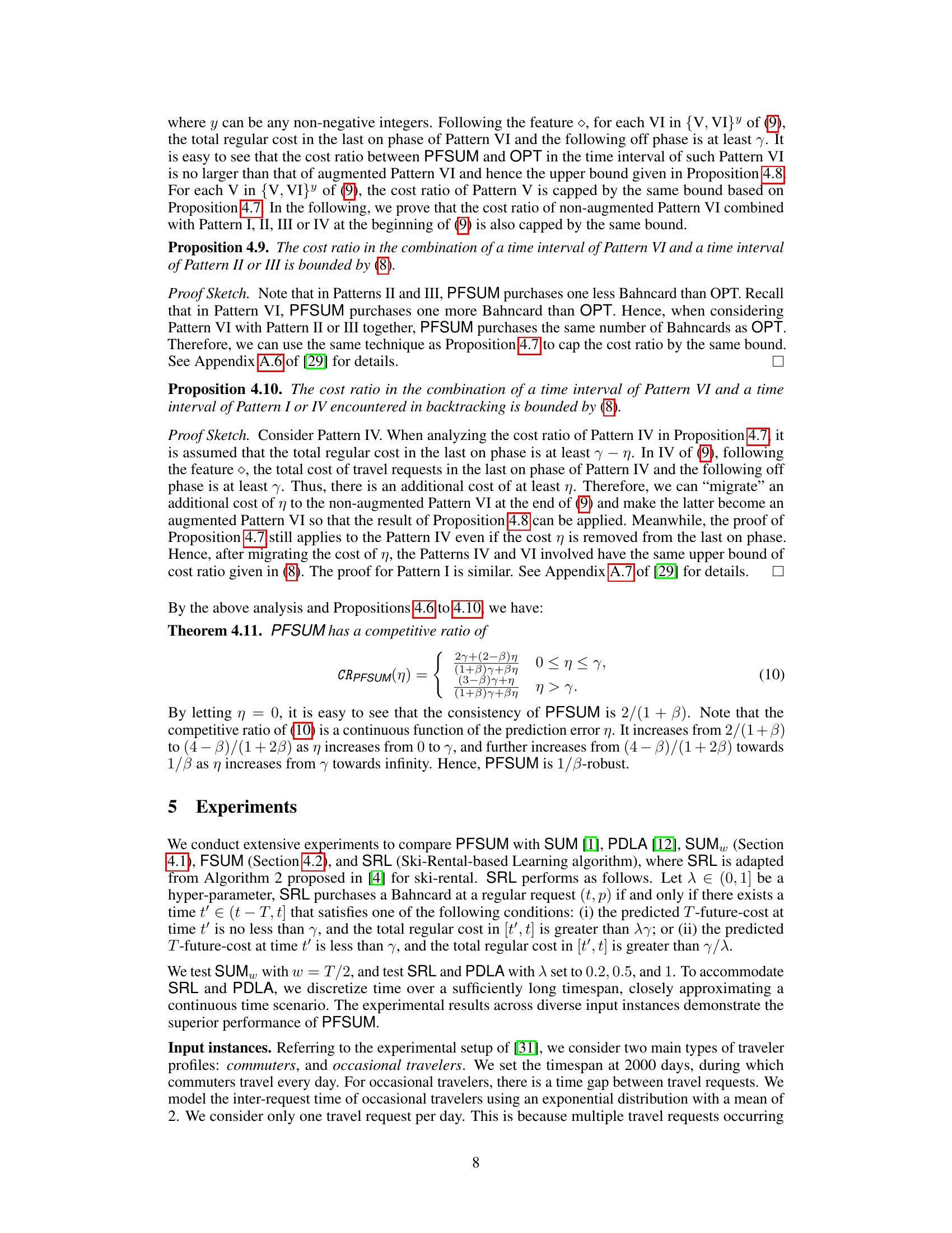
This figure compares the performance of several algorithms for the Bahncard problem in the context of commuters. The x-axis represents the perturbing probability (noise in predictions), and the y-axis represents the average cost ratio. Three different ticket price distributions (Uniform, Normal, and Pareto) are shown. The algorithms compared include SUM, FSUM, SUMw, PFSUM, PDLA (with different λ values), and SRL (with different λ values). The shaded area represents 95% confidence intervals.

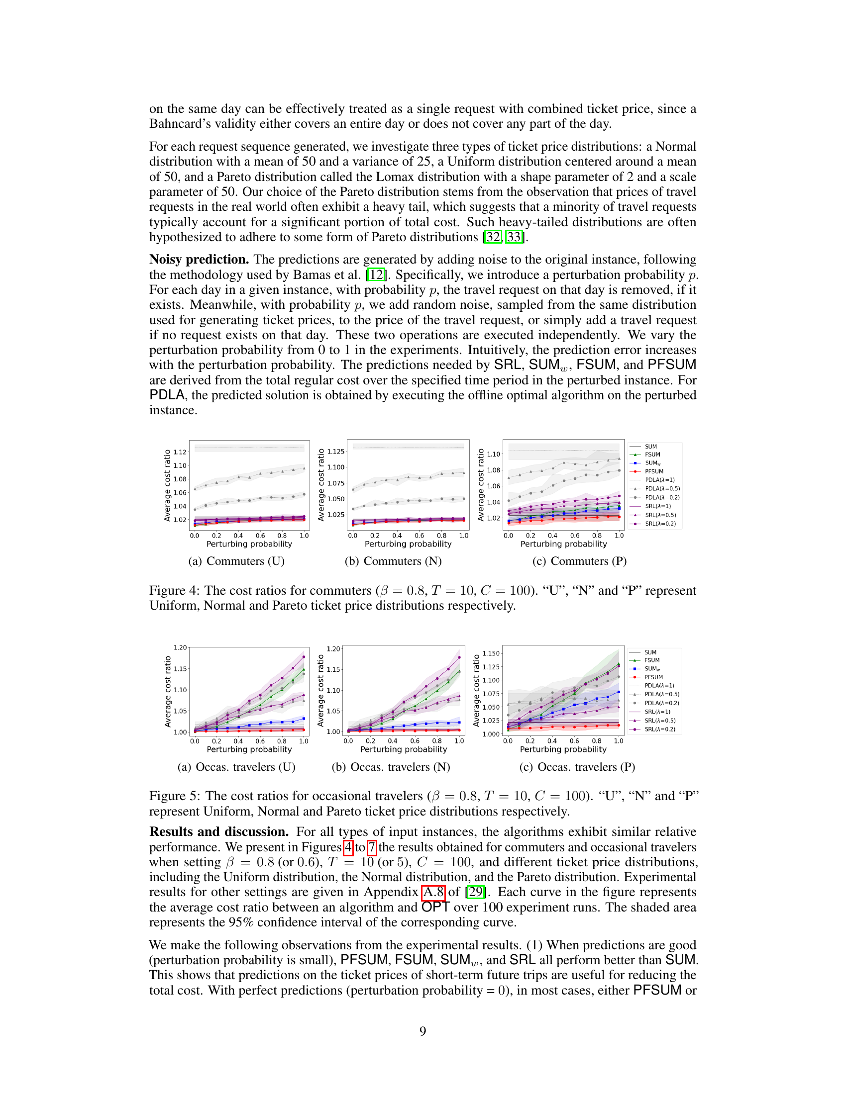
This figure presents the results of experiments conducted to evaluate the performance of different algorithms for occasional travelers using three different ticket price distributions: Uniform, Normal, and Pareto. The x-axis represents the perturbation probability (noise added to predictions), and the y-axis represents the average cost ratio of each algorithm against an optimal offline algorithm. The shaded area shows the 95% confidence interval. The goal is to show how the algorithms’ performance changes under different levels of prediction noise.

This figure shows the average cost ratio for different algorithms (SUM, PFSUM, SUMw, FSUM, PDLA, SRL) with different prediction error levels (perturbation probability). The cost ratio is calculated as the ratio of the cost of the online algorithm to the cost of the optimal offline algorithm. Three different ticket price distributions (Uniform, Normal, Pareto) are considered.

This figure compares the performance of different algorithms in the Bahncard problem for occasional travelers under different ticket price distributions (Uniform, Normal, and Pareto). The x-axis represents the perturbation probability (noise level in the prediction), and the y-axis represents the average cost ratio (algorithm cost / optimal cost). The shaded area shows the 95% confidence interval. It demonstrates the relative cost-effectiveness of the algorithms across varying prediction accuracy and distribution types.

This figure shows an example to illustrate that the consistency of SUMw is at least (3-β)/(1+β). It shows the travel request sequence, the valid time of the Bahncard purchased by SUMw and OPT, and the total cost. The figure demonstrates a scenario where SUMw makes suboptimal decisions due to its cost consideration focusing only on the past and predicted costs.

This figure illustrates six patterns of time intervals where either PFSUM or OPT has a valid Bahncard. The intervals are categorized based on the overlap of Bahncard validity periods between PFSUM and OPT. Patterns I to VI show different scenarios of how the Bahncard purchase times and validities of PFSUM and OPT interact, with ‘x’ representing the number of Bahncards purchased by OPT within a specific time range. Understanding these patterns is crucial for analyzing the competitive ratio of PFSUM.

This figure illustrates six patterns of time intervals where at least one of PFSUM and OPT has a valid Bahncard. The patterns are categorized based on how the Bahncard validity periods of PFSUM and OPT overlap. The key difference highlighted is the variable ‘x’, representing the number of Bahncards purchased by OPT during an ‘on’ phase that expire in the subsequent ‘on’ phase. This variable helps in analyzing the cost ratio between PFSUM and OPT across different scenarios.

This figure illustrates six different patterns of time intervals where either PFSUM or OPT (the optimal offline algorithm) has a valid Bahncard. The intervals are categorized based on the overlap between PFSUM’s and OPT’s Bahncard validity periods. Patterns I-VI represent various scenarios, including complete overlap (Pattern I), no overlap (Pattern II), and partial overlaps starting and ending in different phases (on or off, Patterns III-VI). The variable ‘x’ in Patterns III-VI represents the number of Bahncards OPT purchases in one on phase that expire in a subsequent on phase.

This figure illustrates six different patterns of time intervals where either PFSUM or OPT (the optimal offline algorithm) holds a valid Bahncard. The intervals are analyzed to determine the competitive ratio of PFSUM. Pattern I shows complete overlap between PFSUM and OPT Bahncard validity periods. Patterns II-VI show various scenarios of overlap and non-overlap between PFSUM and OPT Bahncard periods, with ‘x’ representing the number of Bahncards purchased by OPT within a specific pattern.

This figure illustrates six different patterns of time intervals where either PFSUM or OPT (optimal offline algorithm) has a valid Bahncard. The intervals are categorized based on the overlap and positioning of Bahncard validity periods for both algorithms. Pattern I shows a complete overlap, while Patterns II through VI represent various degrees of overlap and placement, with ‘x’ representing the number of Bahncards purchased by OPT during an ‘on’ phase and expiring in a subsequent ‘on’ phase. This categorization is crucial for the divide-and-conquer analysis of PFSUM’s competitive ratio.
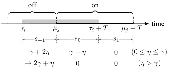
This figure illustrates Lemma 4.4, which discusses the cost ratio between PFSUM and OPT. The shaded area shows the Bahncard’s validity period purchased by OPT. The figure shows three phases: an on phase where OPT has a Bahncard, an off phase where neither OPT nor PFSUM has a Bahncard, and another on phase where OPT has a Bahncard. The lemma analyzes the total regular costs (s2, s3, s4) in these phases to establish an upper bound on the cost ratio.

This figure illustrates six different patterns of time intervals where either PFSUM or OPT (optimal offline algorithm) has a valid Bahncard. These patterns are used in the analysis of the competitive ratio of PFSUM. Pattern I shows a complete overlap of Bahncard validity between PFSUM and OPT. Patterns II through VI depict scenarios where the Bahncard validity intervals overlap partially, with varying degrees of overlap and timing differences. The ‘x’ variable in Patterns III-VI represents the number of Bahncards OPT purchases during a particular time segment. These patterns are crucial to the divide-and-conquer approach used in the paper to analyze the competitive ratio of PFSUM.

This figure illustrates Lemma 4.4, which discusses the cost analysis of the PFSUM algorithm. It shows a timeline divided into an ‘on’ phase (when a Bahncard is valid) and an ‘off’ phase (when no Bahncard is valid). A Bahncard is purchased by the optimal offline algorithm (OPT) at some point. The shaded area represents the duration the OPT’s Bahncard is valid. The figure depicts how the costs (s2, s3, s4) in different segments of the timeline are used in the Lemma’s proof, particularly focusing on the scenario where the T-future cost (c(σ;[t, t+T)) < γ and providing bounds related to the costs when 0 ≤ η ≤ γ and when η > γ, where η is the maximum prediction error.

This figure illustrates six different patterns of time intervals where either PFSUM or OPT (the optimal offline algorithm) has a valid Bahncard. Each pattern shows the relative timing of Bahncard purchases by both algorithms. The key feature is the variable ‘x’ in patterns III-VI, which represents the number of Bahncards purchased by OPT within a specific time window and impacting the overall cost comparison between the two algorithms.

This figure illustrates Lemma 4.4, which discusses the total regular cost in a time interval that overlaps with an off phase. The figure shows a timeline divided into on and off phases representing when a Bahncard is valid for PFSUM and OPT. The shaded rectangle indicates the valid period of a Bahncard purchased by OPT. The labels s2, s3, and s4 represent the total regular costs in the preceding on phase, the off phase, and the succeeding on phase, respectively. The Lemma demonstrates an upper bound on the sum of these costs (s2 + s3 + s4) under certain conditions.

This figure illustrates six different patterns of time intervals where either PFSUM or OPT (an optimal offline algorithm) has a valid Bahncard. The intervals are categorized based on how the valid periods of Bahncards purchased by PFSUM and OPT overlap. Patterns III through VI show scenarios where OPT purchases multiple Bahncards within a longer time frame, impacting the comparison of PFSUM’s performance against OPT. The variable ‘x’ represents the number of Bahncards purchased by OPT during these overlapping periods.

This figure illustrates six patterns of time intervals where at least one of the two algorithms (PFSUM and OPT) has a valid Bahncard. The patterns are categorized based on how the Bahncard validity periods of PFSUM and OPT overlap. Pattern I shows complete overlap, while Patterns II through VI show various partial overlaps. The variable ‘x’ represents the number of Bahncards purchased by OPT during specific overlapping phases, providing further detail on the timing of Bahncard purchases by OPT relative to PFSUM.

This figure illustrates six different patterns of time intervals where either PFSUM or OPT (an optimal offline algorithm) possesses a valid Bahncard. The patterns categorize how the Bahncard validity periods of PFSUM and OPT overlap. Pattern I shows complete overlap, while patterns II through VI show various degrees of partial overlap. The variable ‘x’ represents the number of Bahncards purchased by OPT during specific overlapping scenarios, providing a more nuanced understanding of the cost comparisons between the two algorithms.

This figure illustrates six patterns of time intervals where either PFSUM or OPT (an optimal offline algorithm) has a valid Bahncard. Each pattern represents different combinations of when each algorithm purchases Bahncards and their validity periods. The patterns are essential for analyzing the competitive ratio of PFSUM in the paper. The variable ‘x’ in patterns III-VI represents the number of Bahncards purchased by OPT within a specific timeframe and is crucial for the analysis of these patterns.

This figure compares the performance of various algorithms for the Bahncard problem under different ticket price distributions (Uniform, Normal, and Pareto) for commuter scenarios. The x-axis shows the perturbing probability, representing the level of prediction error, and the y-axis shows the average cost ratio compared to an optimal offline algorithm. The lines represent different algorithms: SUM, FSUM, SUMw, PFSUM, PDLA (with different λ values), and SRL (with different λ values). The shaded areas show 95% confidence intervals.

The figure shows the result of the experiment for commuters with β=0.8, T=10, C=100, and three different ticket price distributions (Uniform, Normal, and Pareto). The x-axis represents the perturbation probability, which simulates prediction error. The y-axis represents the average cost ratio of different algorithms compared to the optimal offline algorithm (OPT). Each line represents a different algorithm (SUM, FSUM, SUMw, PFSUM, PDLA with different λ values, and SRL with different λ values). The shaded area shows the 95% confidence interval for each algorithm.

This figure compares the performance of different algorithms for the Bahncard problem in a commuter setting with various ticket price distributions (Uniform, Normal, and Pareto). The x-axis represents the ‘perturbing probability’, which simulates the accuracy of predictions used by the algorithms. The y-axis shows the average cost ratio, which is the ratio of the algorithm’s total cost to the optimal offline cost. The lower the ratio, the better the algorithm’s performance. The shaded regions represent 95% confidence intervals.

This figure compares the performance of different algorithms (SUM, FSUM, SUMw, PFSUM, PDLA, SRL) for occasional travelers using three different ticket price distributions (Uniform, Normal, Pareto). The x-axis represents the perturbing probability, which reflects the prediction error. The y-axis represents the average cost ratio of each algorithm against OPT (optimal offline algorithm). The shaded areas denote the 95% confidence intervals.

The figure shows the performance comparison of various algorithms for commuters, with beta=0.8, T=10, and C=100 under different ticket price distributions: Uniform, Normal, and Pareto. Each distribution is represented by a subplot, and the x-axis shows the perturbing probability (noise level in prediction) while the y-axis indicates the average cost ratio. The shaded area shows the 95% confidence interval.

This figure shows the average cost ratios for occasional travelers using different algorithms under three ticket price distributions: Uniform, Normal, and Pareto. The x-axis represents the perturbing probability, which simulates the prediction error, ranging from 0 to 1. The y-axis shows the average cost ratio, comparing the cost of each algorithm to the optimal offline algorithm (OPT). The shaded area represents the 95% confidence interval.
Full paper#
