↗ OpenReview ↗ NeurIPS Homepage ↗ Hugging Face ↗ Chat
TL;DR#
Current large pre-trained models struggle with multivariate time series forecasting due to high computational costs and slow inference. Smaller models offer resource efficiency but often lack accuracy in zero/few-shot scenarios. The challenge lies in developing accurate and efficient models for diverse real-world datasets.
This paper introduces Tiny Time Mixers (TTM), small yet powerful pre-trained models for improved multivariate time series forecasting. TTM utilizes a lightweight architecture and incorporates innovations such as adaptive patching, diverse resolution sampling, and resolution prefix tuning to handle varied dataset resolutions with minimal model capacity. It outperforms current benchmarks in zero/few-shot forecasting by a significant margin (4-40%), while being extremely resource-efficient, and suitable for deployment even on CPU-only machines.
Key Takeaways#
Why does it matter?#
This paper is crucial for researchers in time series forecasting due to its introduction of Tiny Time Mixers (TTM), a novel lightweight model. TTM addresses the limitations of existing large models by offering enhanced zero/few-shot forecasting capabilities with significantly reduced computational demands. Its resource efficiency makes it easily deployable in constrained environments and paves the way for more efficient pre-trained models in time series analysis. The research also opens avenues for further investigation in multi-level modeling, adaptive patching, and resolution prefix tuning for improving the efficiency and generalization of small pre-trained models.
Visual Insights#
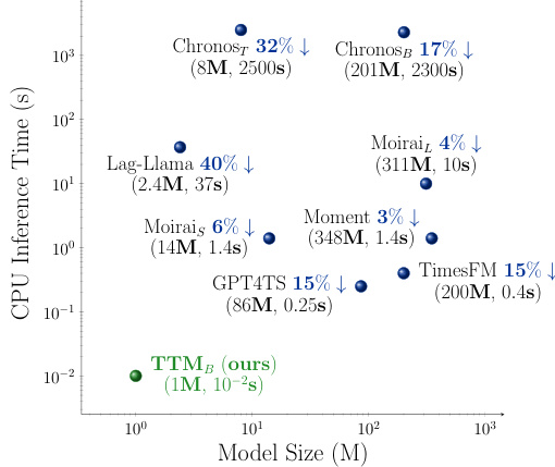
This figure compares the Tiny Time Mixer (TTM) model with other state-of-the-art (SOTA) pre-trained time series models in terms of model size and CPU inference time. It shows that TTM significantly outperforms the SOTAs in terms of accuracy while being much smaller and faster. The X% values indicate the percentage improvement of TTM over each benchmark model in terms of forecasting accuracy.
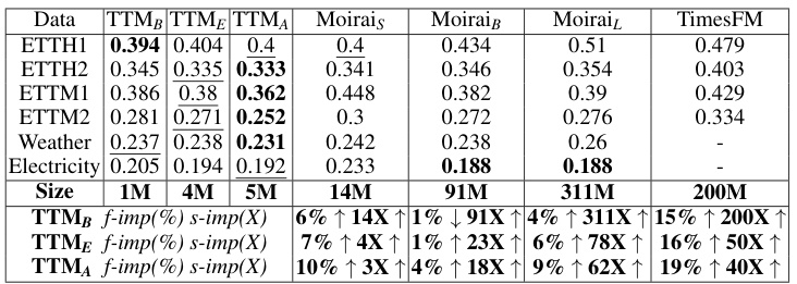
This table presents the zero-shot forecast improvement and model size improvement of the Tiny Time Mixers (TTM) model compared to two state-of-the-art (SOTA) models, Moirai and TimesFM. The improvement is measured by mean squared error (MSE) across various forecast lengths (FL). Note that some results for TimesFM are missing because the data used for those specific results were also used in its pre-training.
In-depth insights#
Tiny Time Mixers#
The concept of “Tiny Time Mixers” in the context of time series forecasting is intriguing. It suggests a paradigm shift towards smaller, more efficient models that rival the performance of much larger, computationally expensive counterparts. The “tiny” aspect emphasizes resource efficiency, making these models suitable for deployment on resource-constrained devices. The “time mixer” component likely refers to the model’s architecture, which is designed to effectively capture temporal dynamics and relationships within multivariate time series data. The effectiveness of such models hinges on the transfer learning capabilities; they likely use a pre-training phase on a large dataset to acquire a robust representation that generalizes to downstream, zero or few-shot forecasting tasks. This approach would greatly reduce training time and computational costs while maintaining prediction accuracy. Overall, “Tiny Time Mixers” presents a promising direction for practical multivariate time series forecasting, emphasizing efficiency and accessibility without sacrificing performance.
Multi-Level Modeling#
The concept of “Multi-Level Modeling” in the context of time series forecasting, as described in the provided research paper, signifies a powerful strategy for enhancing model performance. By adopting a hierarchical architecture, it allows for the effective capture of both local (short-term) and global (long-term) patterns within the data. This multi-level approach involves distinct components, each designed to handle specific aspects of the data, such as channel-independent feature extraction and subsequent channel-mixing. This division of labor leads to increased efficiency. The use of a lightweight architecture, like TSMixer, enhances the speed and scalability of the model, making it particularly suitable for real-world applications with resource constraints. The combination of adaptive patching and diverse resolution sampling ensures robustness and adaptability across diverse datasets, effectively leveraging transfer learning capabilities. Ultimately, the multi-level design promotes effective feature fusion, leading to improved forecasting accuracy, especially in the zero-shot and few-shot scenarios.
Pre-training Enhancements#
The paper significantly enhances the pre-training process by introducing three key innovations: Adaptive Patching (AP), which dynamically adjusts patch lengths across different layers of the model to better handle the heterogeneous nature of diverse time-series datasets; Diverse Resolution Sampling (DRS), which augments pre-training data by incorporating diverse sampling rates to improve generalization across various resolutions; and Resolution Prefix Tuning (RPT), which explicitly embeds resolution information into the model’s input to facilitate resolution-conditioned modeling. These enhancements collectively enable efficient pre-training of small-scale models on a large-scale dataset containing varied time-series data, demonstrating the power of resource-efficient transfer learning for time-series forecasting.
Zero-shot Forecasting#
Zero-shot forecasting, a significant advancement in time series analysis, focuses on a model’s ability to predict unseen data without prior training on that specific data. This capability is highly valuable because it reduces the need for extensive labeled datasets which are often scarce and costly to acquire, especially for multivariate time series. The core idea is transfer learning: leveraging knowledge gained from training on diverse datasets to effectively predict new, related time series. However, the success of zero-shot forecasting hinges on the model’s architecture and pre-training strategy. A well-designed model, such as a transformer-based or MLP-Mixer model, coupled with a comprehensive pre-training dataset, can greatly improve forecasting accuracy. This technique is particularly beneficial for scenarios where obtaining sufficient labeled data is impractical or expensive, making it crucial for real-world applications dealing with multivariate time series and limited resources.
Future Work#
The authors outline several promising avenues for future research. Extending TTM’s capabilities beyond forecasting is a key goal, aiming to incorporate tasks such as classification, regression, and anomaly detection. This expansion would significantly broaden the model’s applicability across diverse domains. Addressing TTM’s sensitivity to context length is another priority. The current model requires separate training for different context lengths, limiting its flexibility. Future work will focus on developing more adaptable architectures capable of handling varying context lengths dynamically. Finally, enhancing TTM to support probabilistic forecasting is highlighted. Currently, TTM focuses on point forecasts, which would be significantly improved through the incorporation of distribution heads to provide more robust predictions.
More visual insights#
More on figures
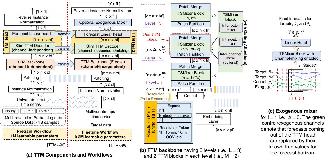
This figure provides a comprehensive overview of the Tiny Time Mixer (TTM) model architecture and workflow. It is divided into three parts: (a) illustrates the components and workflows of TTM. It shows a multi-level architecture with a backbone for feature extraction, a decoder for channel correlation and exogenous signal handling, and a head for forecasting. (b) details the TTM backbone architecture. It explains how the backbone uses adaptive patching, diverse resolution sampling, and resolution prefix tuning to handle varied dataset resolutions. (c) shows how exogenous information is incorporated into the forecasting process using an exogenous mixer. In summary, this figure provides a detailed view of the TTM model’s design, showing how it combines various components and techniques to achieve efficient and accurate multivariate time series forecasting.

This figure provides a comprehensive overview of the Tiny Time Mixer (TTM) model architecture and workflow. Panel (a) illustrates the main components of the TTM model: the backbone, decoder, forecast head, and optional exogenous mixer. It also depicts the pre-training and fine-tuning workflows. Panel (b) details the architecture of the TTM backbone, which consists of multiple levels and blocks of TSMixer units. Adaptive patching, diverse resolution sampling, and resolution prefix tuning are highlighted as key features for handling multi-resolution data. Panel (c) explains the exogenous mixer, which fuses exogenous data into the forecasting process to capture channel correlations and exogenous signals.
This figure compares the performance of Tiny Time Mixers (TTMB) against other open-source pre-trained time series models. It shows the model size (in millions of parameters) plotted against inference time (per batch in seconds) on a logarithmic scale. Each point represents a different model, and the percentage values near each point indicate the relative performance improvement of TTMB compared to that specific model. The figure highlights that TTMB achieves comparable or higher accuracy with a smaller model size and much faster inference time, thus being more efficient.

This figure compares the model size and inference time of the proposed Tiny Time Mixer (TTM) model against other state-of-the-art (SOTA) pre-trained time series forecasting models. It shows that TTM achieves comparable accuracy with a significantly smaller model size and faster inference time. The X% values represent the accuracy improvement of TTM over the other models.
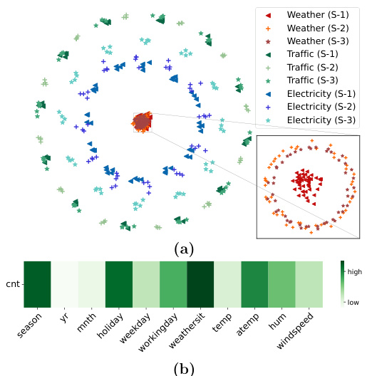
This figure visualizes the TTM embeddings from various datasets (weather, traffic, and electricity) using PCA projection. Each dataset is represented by a different color. From each dataset, three distant, non-overlapping, fixed-length time segments (S-1, S-2, S-3) are selected, each depicted with a unique marker shape. The visualization uses the first and second principal components of the TTM embeddings. The inset image focuses on the weather dataset alone, revealing a deeper structure learned by the TTM architecture. The cyclic orbits in the embeddings reflect the seasonal patterns in the data. Both hourly datasets (traffic and electricity) form concentric orbits due to similar seasonal patterns, while the weather data, with its distinct seasonal pattern, shows cyclic orbits in a different sub-dimension. In addition, the cross-channel attention from the fine-tuned model’s channel mixing layers reveals feature importance across channels. As shown, the model focuses on channels like weathersit, season, holiday, and temperature to predict bike-rental counts. These attention model weights correlate with the general data characteristics where bike rental demands are heavily influenced by weather and holidays, providing explanation for the fine-tuned model predictions.
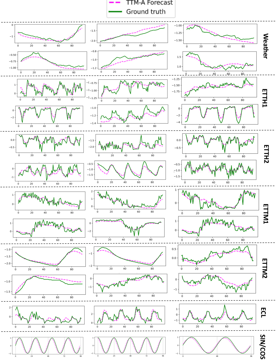
This figure provides a comprehensive overview of the Tiny Time Mixer (TTM) model architecture and workflow. It’s broken down into three subfigures: (a) Shows the TTM components and workflows including the backbone, decoder, forecast head, and exogenous mixer. It also illustrates the pre-training and fine-tuning workflows. (b) Details the architecture of the TTM backbone. It consists of multiple levels and blocks which allow for mixing of features within patches, across patches and channels. It highlights elements such as adaptive patching, diverse resolution sampling, and resolution prefix tuning. (c) Illustrates the exogenous mixer which combines the model’s forecasts with known exogenous values, enabling the model to integrate external information into the forecast predictions.

This figure compares Tiny Time Mixer (TTMB) with other state-of-the-art (SOTA) pre-trained time series models in terms of model size, inference time, and forecasting accuracy. Each model is represented by a point on a scatter plot where the x-axis represents model size (in millions of parameters) and the y-axis represents CPU inference time (in seconds). The percentage value next to each SOTA model indicates how much less accurate its forecast is compared to TTMB’s. The figure clearly demonstrates the superior performance of TTMB in terms of efficiency and accuracy.

This figure visualizes the TTM embeddings from various datasets (weather, traffic, and electricity) using PCA projection. Each dataset is represented by a different color. From each dataset, three distant, non-overlapping, fixed-length time segments (S-1, S-2, S-3) are selected, each depicted with a unique marker shape. The visualization uses the first and second principal components of the TTM embeddings. The inset image focuses on the weather dataset alone, revealing a deeper structure learned by the TTM architecture. The cyclic orbits in the embeddings reflect the seasonal patterns in the data. Both hourly datasets (traffic and electricity) form concentric orbits due to similar seasonal patterns, while the weather data, with its distinct seasonal pattern, shows cyclic orbits in a different sub-dimension. In addition, the cross-channel attention from the fine-tuned model’s channel mixing layers reveals feature importance across channels. As shown, the model focuses on channels like weathersit, season, holiday, and temperature to predict bike-rental counts. These attention model weights correlate with the general data characteristics where bike rental demands are heavily influenced by weather and holidays, providing explanation for the fine-tuned model predictions.
More on tables
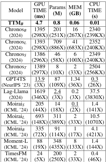
This table compares the computational efficiency of TTM against other state-of-the-art time series forecasting models. It shows the inference time per batch (both on GPU and CPU), the number of parameters, and the maximum GPU memory usage for each model. The significant reduction in computational resources required by TTM is highlighted by the scaling factors (nX) indicating how much faster and more memory efficient TTM is compared to the other models.

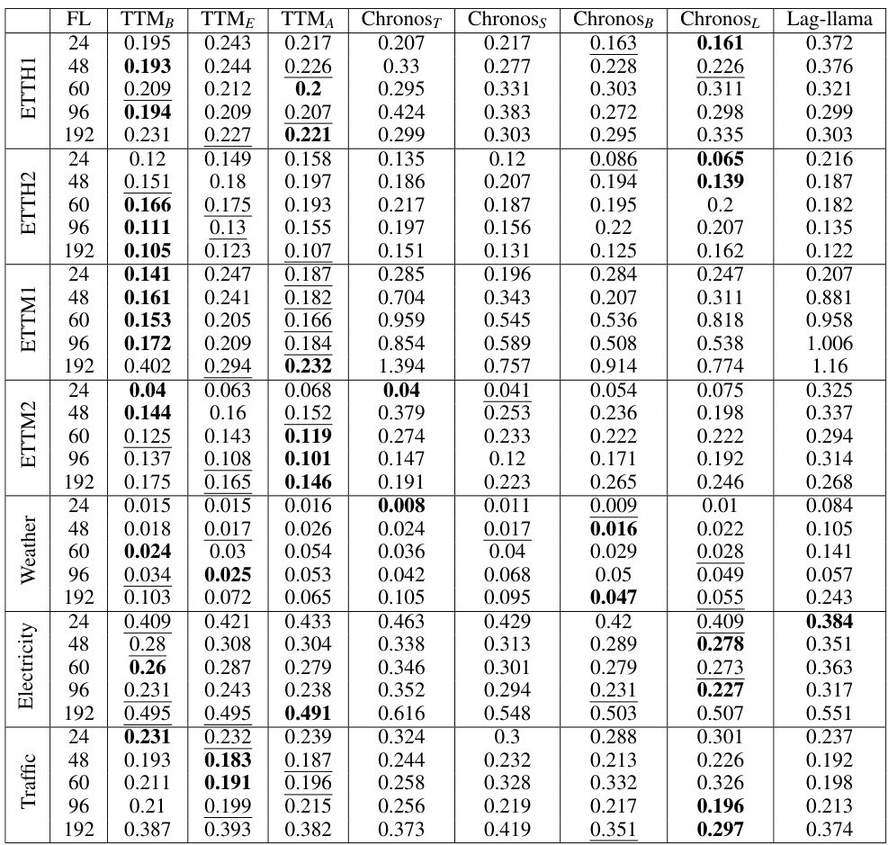
This table compares the zero-shot forecasting performance of three variants of the Tiny Time Mixer (TTM) model against Chronos and Lag-Llama models. It shows the improvement in Mean Squared Error (MSE) and model size reduction achieved by TTM compared to the baselines across different forecast lengths. The results highlight TTM’s superior performance and efficiency.

This table shows the results of a few-shot learning experiment (5% of training data used for fine-tuning) comparing TTM against several other state-of-the-art forecasting models. It evaluates the performance on multiple datasets (ETTH1, ETTH2, ETTM1, ETTM2, Weather, Electricity, Traffic) across various forecast lengths (FL). The table highlights TTM’s superior performance even with limited training data by showing the percentage improvement over other models.
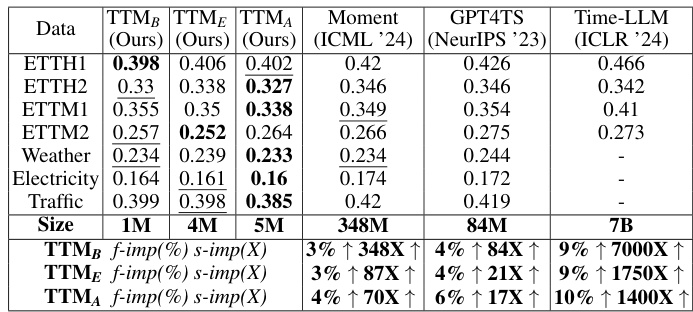
This table compares the performance of three variants of the Tiny Time Mixer (TTM) model against two state-of-the-art (SOTA) multivariate time series forecasting models, Moirai and TimesFM, in a zero-shot setting. It shows the percentage improvement in Mean Squared Error (MSE) and the size improvement (ratio of baseline model size to TTM model size) achieved by each TTM variant. Note that some results for comparison models are missing due to the pre-training data used.

This table lists the datasets used for pre-training the TTM model. It shows the source of each dataset (Monash or LibCity), the dataset name, and the resolutions (sampling frequencies) available for each. The ‘+ Downsample’ annotation indicates that the Diverse Resolution Sampling (DRS) technique was applied to generate additional datasets with lower resolutions than the original. Importantly, these pre-training datasets are distinct from the evaluation datasets used later in the paper. The last three LibCity datasets were excluded from the pre-training used for enterprise releases of the model.
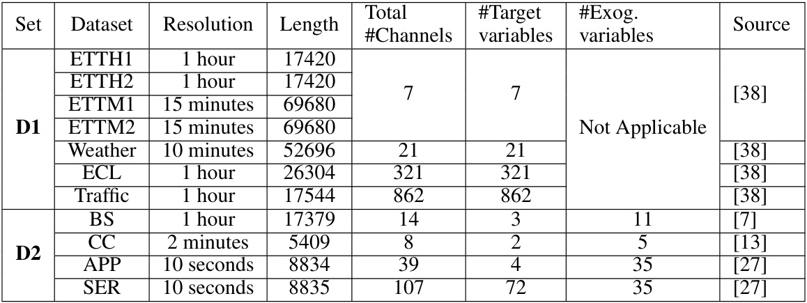
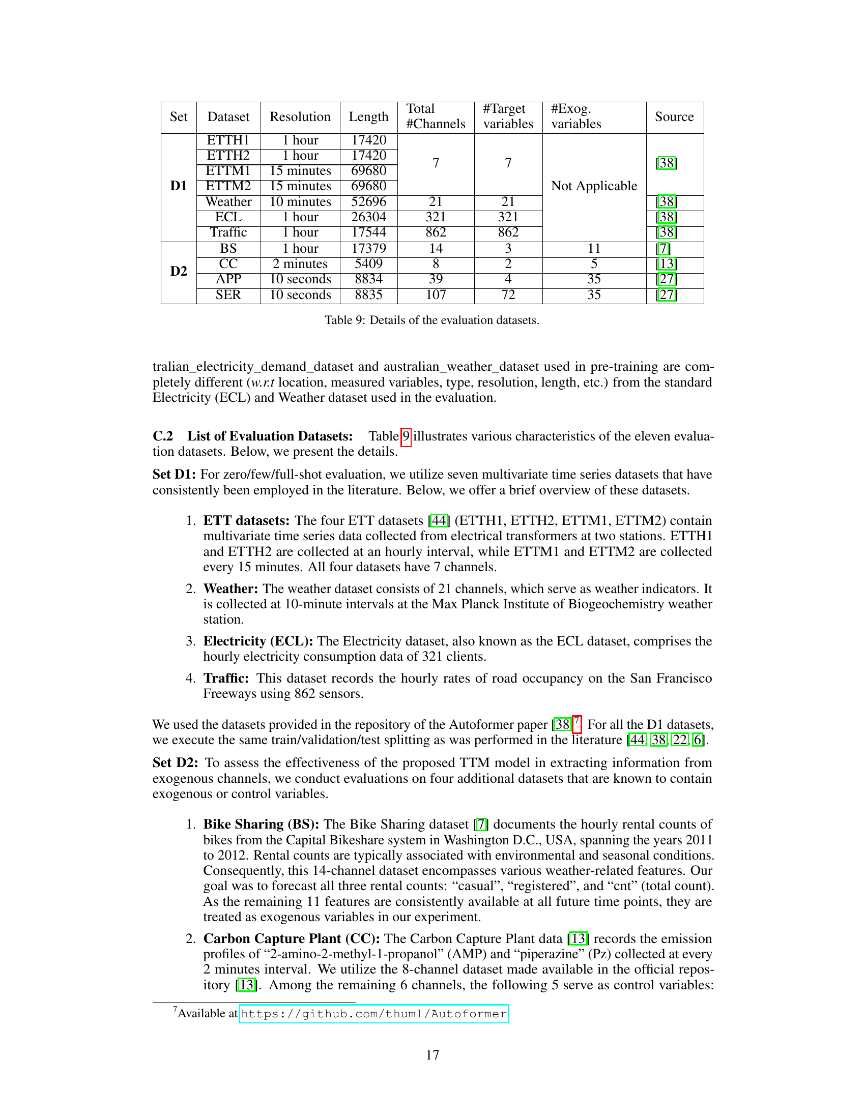
This table lists eleven datasets used for evaluating the performance of the proposed TTM model. It provides details for each dataset including the name, resolution (sampling frequency), length of the time series, the total number of channels, the number of target variables (channels for which forecasts are required), and the number of exogenous variables (optional channels influencing the forecasts). The datasets are categorized into two sets: D1 and D2. D1 datasets are commonly used benchmarks for multivariate time series forecasting, while D2 datasets are included to evaluate the effectiveness of handling exogenous variables and channel correlations within the TTM model.

This table compares the zero-shot forecast performance and model size of three TTM variants (TTMB, TTME, TTMA) against two state-of-the-art time series forecasting models, Moirai and TimesFM. It shows the percentage improvement in MSE and the ratio of the baseline model size to the TTM model size, demonstrating that TTM achieves superior accuracy with significantly smaller model size. Note that some results are omitted because the baseline models used that data for pre-training.
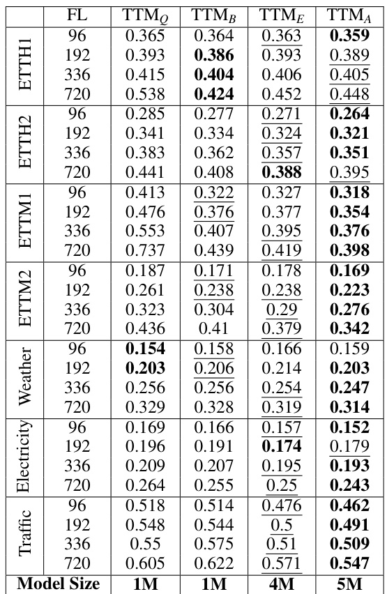
This table presents the zero-shot forecasting performance of different TTM variants (TTM0, TTMB, TTME, TTMA) on seven datasets (ETTH1, ETTH2, ETTM1, ETTM2, Weather, Electricity, Traffic). The results are reported for four forecast lengths (FLs): 96, 192, 336, and 720. The table allows for comparison of model performance across different forecast horizons and datasets using the standard test protocol which employs a sliding window approach.

This table presents the zero-shot forecasting performance of different TTM model variants (TTM0, TTMB, TTME, TTMA) across various forecast lengths (FL) on seven datasets (ETTH1, ETTH2, ETTM1, ETTM2, Weather, Electricity, Traffic). The results are averaged across all sliding windows, representing the mean squared error (MSE) for each model and forecast length combination on each dataset.
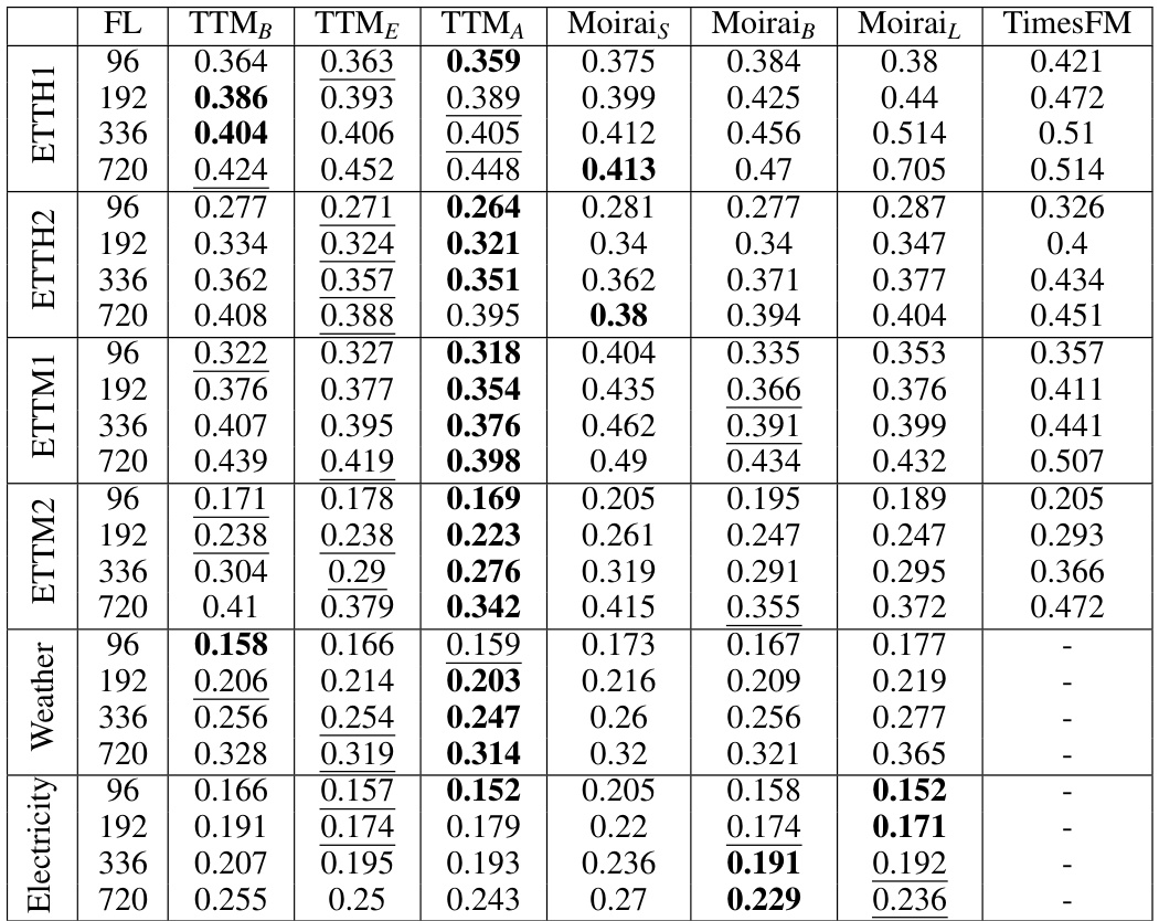
This table presents the Mean Squared Error (MSE) values achieved by different variants of the Tiny Time Mixer (TTM) model in a zero-shot setting. The results are shown for various forecast lengths (FL) across several evaluation datasets (D1) using the standard test protocol, which involves using all sliding test windows. This demonstrates TTM’s performance compared to other models without any fine-tuning on the target datasets.

This table presents the zero-shot forecast improvement and model size improvement of the Tiny Time Mixers (TTM) models compared to the Moirai and TimesFM models. The results show that TTM significantly outperforms existing benchmarks while using substantially fewer parameters. The MSE is averaged across various forecast lengths (FLs). Note that some results from TimesFM and Moirai are missing because these models used the respective datasets for pre-training.
This table compares the zero-shot forecast performance and model size of three variants of the Tiny Time Mixer (TTM) model against two state-of-the-art (SOTA) models, Moirai and TimesFM. It shows the percentage improvement in Mean Squared Error (MSE) achieved by each TTM variant compared to Moirai and TimesFM, along with the ratio of the SOTA model size to the TTM model size. The results are averaged across different forecast lengths (FL). Note that some results for TimesFM are missing due to data overlap between training and evaluation sets.

This table presents the zero-shot results for all TTM variants (TTM0, TTMB, TTME, TTMA) across different forecast lengths (FL) on the D1 benchmark dataset. It shows the Mean Squared Error (MSE) for each model variant across various datasets (Traffic, Electricity, Weather, ETTM2, ETTM1, ETTH2, ETTH1) and forecast lengths, enabling a comprehensive comparison of performance under zero-shot conditions.

This table compares the zero-shot forecasting performance and model size of three variants of the Tiny Time Mixer (TTM) model against two state-of-the-art (SOTA) models, Moirai and TimesFM. It shows the percentage improvement in MSE and the ratio of the SOTA model size to the TTM model size. Note that some results are missing due to data usage in pre-training.

This table presents the results of a 5% few-shot experiment, comparing the performance of different TTM variants (TTM0, TTMB, TTME, and TTMA) against several baseline models across various datasets (ETTH1, ETTH2, ETTM1, ETTM2, Weather, Electricity, and Traffic). The experiment uses all sliding test windows for different forecast lengths. The results are expressed as MSE scores and show TTM variants consistently outperforming the baselines.

This table presents a comparison of the Tiny Time Mixers (TTM) model’s zero-shot forecasting performance against two state-of-the-art (SOTA) models: Moirai and TimesFM. The comparison focuses on forecast improvement percentage (f-imp) and model size improvement (s-imp). The results are averaged across various forecast lengths (FL). Note that some results are missing due to data used in pre-training of the comparison models.

This table compares the zero-shot performance of TTM against LLMTime on four datasets (ETTM2, Weather, Electricity, and Traffic) with two forecast lengths (96 and 192). It shows the MSE values achieved by different TTM variants (TTMB, TTME, and TTMA) and LLMTime. The table also highlights the significant size difference between TTM and LLMTime, illustrating TTM’s superior performance with a substantially smaller model size. The f-imp(%) and s-imp(X) show the percentage improvement in MSE and the size improvement factor compared to LLMTime.
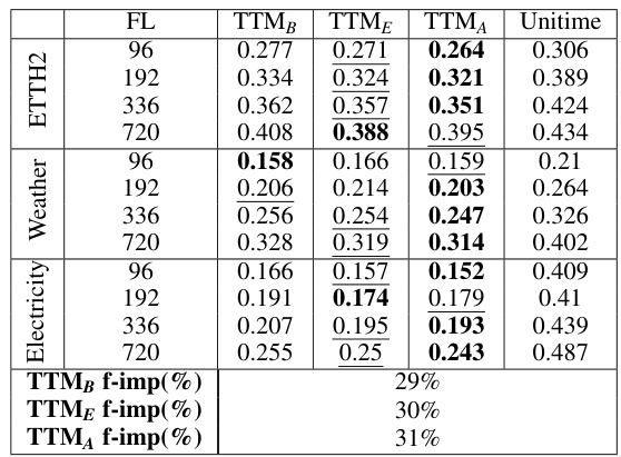
This table compares the performance of TTM models against UniTime models in a zero-shot setting using the full sliding window test set. It shows the mean squared error (MSE) for each model on four datasets (Electricity, Weather, ETTH2, and ETTH1) across four forecast lengths (FLs). The ‘f-imp(%)’ rows show the percentage improvement of each TTM model compared to UniTime. The results demonstrate consistent improvement across the different datasets and forecast horizons, with TTMA exhibiting the largest improvement of 31%.

This table shows the MSE improvement of TTMQ compared to other self-supervised pre-trained models (SimMTM, Ti-MAE, TST, LaST, TF-C, COST, TS2Vec) in different few-shot settings (10%, 25%, 50%, 75%, 100%). The models are initially pre-trained on ETTH2 and then fine-tuned on ETTH1 using the specified percentage of training data. The ‘IMP’ column shows the percentage improvement of TTMQ’s MSE over the baseline model in each setting.

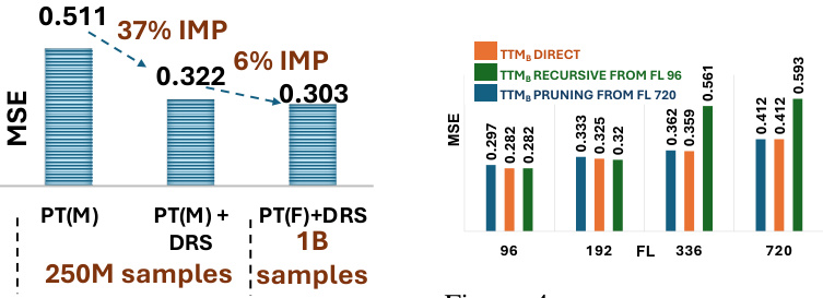
This table presents the impact of adaptive patching (AP) and resolution prefix tuning (RPT) on the performance of the TTM model in zero-shot forecasting with different amounts of pre-training data. The results are reported for the forecast length (FL) of 96, showing the impact of adaptive patching across different amounts of pre-training data. It also shows how resolution prefix tuning enhances the performance especially when there is abundant and diverse pre-training data.
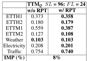
This table shows the impact of Resolution Prefix Tuning (RPT) on the model’s performance when the context length (SL) is short (96). It compares the model’s performance with and without RPT, measured by Mean Squared Error (MSE) on various datasets for a forecast length (FL) of 24. The improvement in MSE (IMP) is calculated and shown as a percentage.
Full paper#


