↗ OpenReview ↗ NeurIPS Homepage ↗ Chat
TL;DR#
Many machine learning models use post-hoc transformations like ensembling or SWA to boost performance. However, these are usually applied after initial model selection, ignoring potential performance shifts. This paper identifies an issue: these transformations can sometimes reverse the performance trends of the base models, particularly in noisy datasets. This challenges the standard model selection practice.
To address this, the authors propose ‘post-hoc selection’. Instead of selecting models based on initial performance, they select based on the performance after post-hoc transforms are applied. This method showed improvement across various datasets and model types. The core idea is that post-hoc transforms might suppress the influence of noisy data, allowing better models to be selected based on more robust metrics.
Key Takeaways#
Why does it matter?#
This paper is crucial because it challenges a common practice in machine learning, demonstrating that post-hoc model transformations can reverse performance trends. This finding necessitates a reevaluation of model selection strategies and opens avenues for improving model development, especially in high-noise settings.
Visual Insights#

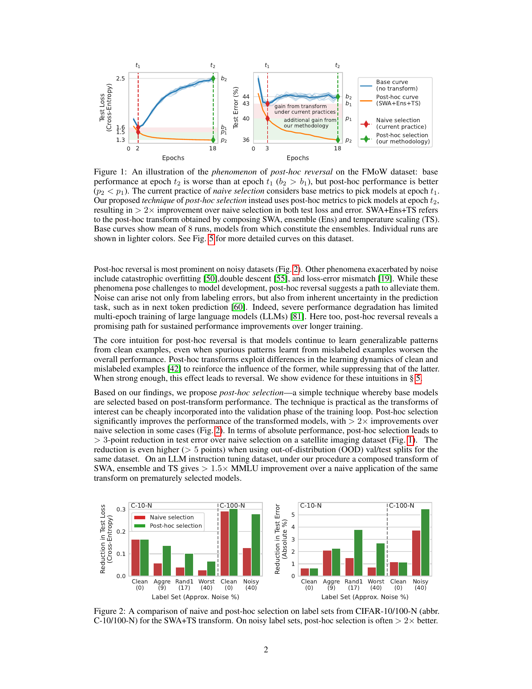
This figure illustrates the concept of post-hoc reversal using the FMoW dataset. It shows that while the base model’s performance is worse at a later epoch (t2), the performance after applying post-hoc transforms (SWA, ensembling, and temperature scaling) is better at the later epoch. This highlights the limitations of naive selection (choosing models based on initial performance) and advocates for post-hoc selection (choosing models based on performance after transforms). The figure compares the performance curves before and after applying the post-hoc transforms.

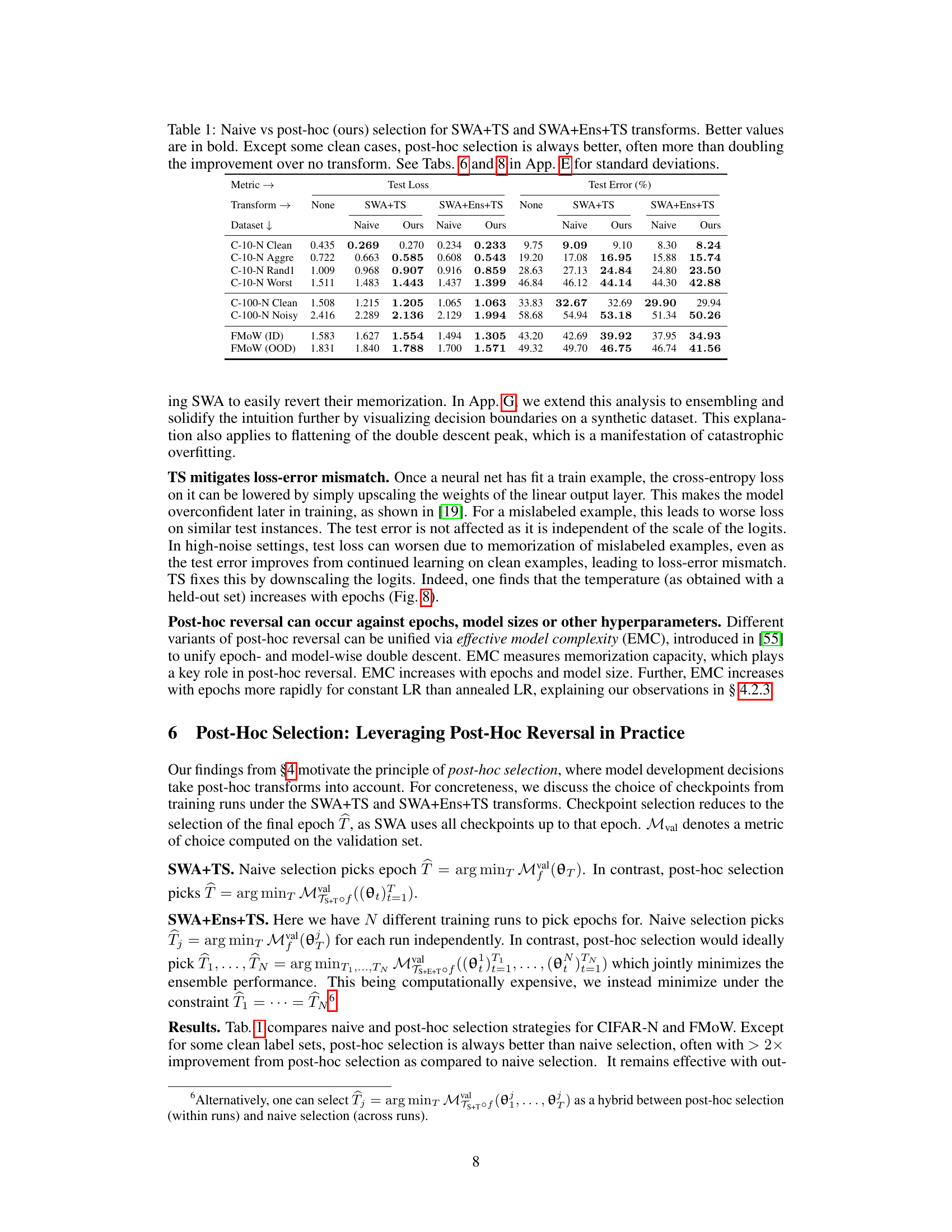
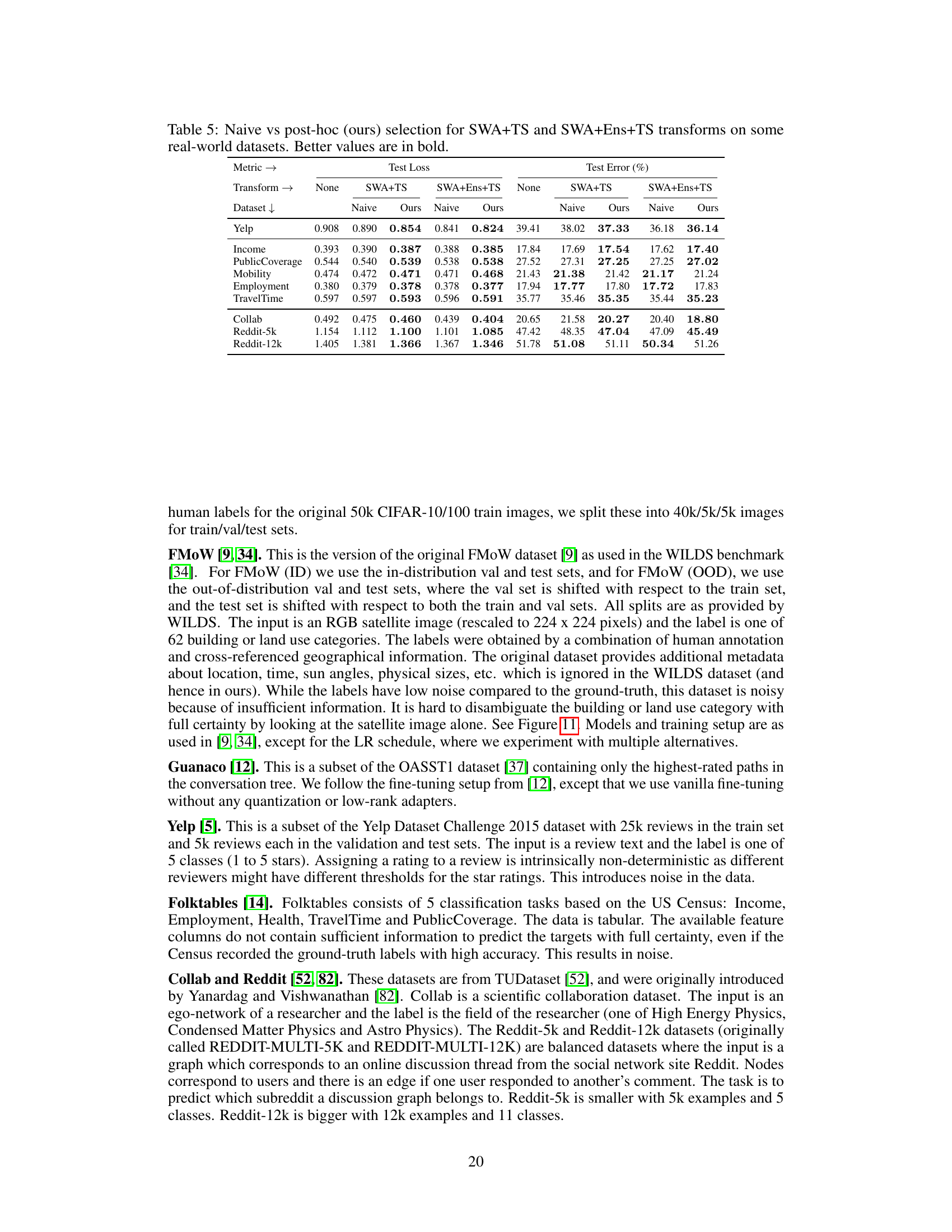
This table compares the performance of naive model selection versus post-hoc model selection using two different post-hoc transformations (SWA+TS and SWA+Ens+TS). Naive selection chooses the best performing model based on its initial performance without any post-hoc transformations. Post-hoc selection instead selects the model based on its performance after applying the chosen post-hoc transformations. Better values (lower test loss and test error) are bolded. The table demonstrates that post-hoc selection consistently outperforms naive selection, often leading to more than double the improvement over not using any transformations. Standard deviations for the results are available in Appendix E.
In-depth insights#
Post-hoc Reversal#
The concept of “Post-hoc Reversal” introduces a phenomenon where performance trends observed in base machine learning models are inverted after applying post-hoc transforms like temperature scaling, ensembling, or stochastic weight averaging. This reversal is particularly pronounced in high-noise scenarios, challenging the conventional practice of selecting models based solely on pre-transform metrics. Post-hoc reversal highlights the limitations of naive model selection and suggests that post-hoc metrics should significantly influence model development decisions, including hyperparameter choices and early stopping. This phenomenon offers a potential method to mitigate issues like catastrophic overfitting and loss-error mismatches commonly associated with noisy datasets. The core intuition behind post-hoc reversal is the differential learning dynamics between clean and mislabeled examples. Post-hoc transforms are effective in suppressing the influence of mislabeled examples while retaining generalizable patterns from clean data, leading to a performance reversal. Therefore, post-hoc selection, a strategy where post-hoc metrics are used to guide model selection, presents a more robust and effective methodology compared to the traditional approach. This technique has demonstrated considerable performance improvement across various domains and model architectures, demonstrating its widespread applicability.
Epoch-wise trends#
Analyzing epoch-wise trends in the context of post-hoc transforms reveals crucial insights into model training dynamics. Early epochs often show poor performance due to noise or overfitting, but post-hoc methods like stochastic weight averaging (SWA) and ensembling can reverse this trend, improving performance in later epochs. This phenomenon, termed post-hoc reversal, highlights the limitations of selecting models based solely on early performance metrics. Post-hoc reversal is particularly pronounced in high-noise settings, where early overfitting is significant. This observation suggests that post-hoc transforms may be more effective at filtering out noisy data, allowing the model to learn generalizable patterns from clean examples. Therefore, evaluating models based on post-hoc performance metrics (rather than early-epoch metrics) is crucial. This approach, termed post-hoc selection, can lead to more robust models with improved generalization abilities. Investigating the learning dynamics and the influence of mislabeled samples across different epochs provides a comprehensive understanding of model behavior, shaping better model development strategies.
Post-hoc Selection#
The proposed “Post-hoc Selection” method offers a compelling alternative to traditional model selection in machine learning. Instead of selecting models based solely on their initial performance metrics, post-hoc selection leverages the performance improvements achieved after applying post-hoc transforms like temperature scaling, ensembling, and stochastic weight averaging. This approach directly addresses the phenomenon of “post-hoc reversal,” where initial performance trends are reversed after these transformations, particularly noticeable in high-noise settings. By prioritizing post-transform performance, post-hoc selection can lead to significant performance gains, even surpassing models that initially appeared superior. This innovative approach improves model development by better accounting for how post-hoc transforms alter the characteristics of the trained models. Its simplicity—integrating directly into the validation phase—and demonstrated effectiveness on various datasets make it a practical and impactful contribution to the field.
Noisy Data Impact#
The impact of noisy data is a central theme, explored through the lens of post-hoc transforms like temperature scaling, ensembling, and stochastic weight averaging. The paper reveals a phenomenon called post-hoc reversal, where performance trends are reversed after applying these transforms, particularly in high-noise scenarios. This implies that selecting models solely based on pre-transform performance (naive selection) can be suboptimal. Noise affects model generalizability; it can exacerbate overfitting, double descent, and mismatches between loss and error. However, the paper’s key insight is that post-hoc transforms can mitigate the negative effects of noise, by selectively suppressing the influence of mislabeled examples while retaining the generalizable patterns learned from clean data. This leads to a recommendation for post-hoc selection, which chooses models based on their post-transform performance, ultimately improving model accuracy and robustness.
Future Directions#
Future research should prioritize developing a deeper theoretical understanding of post-hoc reversal, moving beyond empirical observations to explain its underlying mechanisms. This includes exploring the relationship between post-hoc reversal and model complexity, as well as investigating how different types of noise influence the phenomenon. Developing more sophisticated checkpoint selection strategies is crucial, potentially incorporating ensemble methods or Bayesian approaches to overcome limitations of naive selection. Extending the research to additional domains and modalities will demonstrate the robustness and generalizability of post-hoc reversal. A crucial area of investigation is determining how best to integrate post-hoc transforms into model development workflows, perhaps through automated early stopping methods. Finally, a key future direction involves developing techniques for robustly handling high-noise settings, such as those found in real-world datasets, to maximize the practical benefits of post-hoc selection.
More visual insights#
More on figures

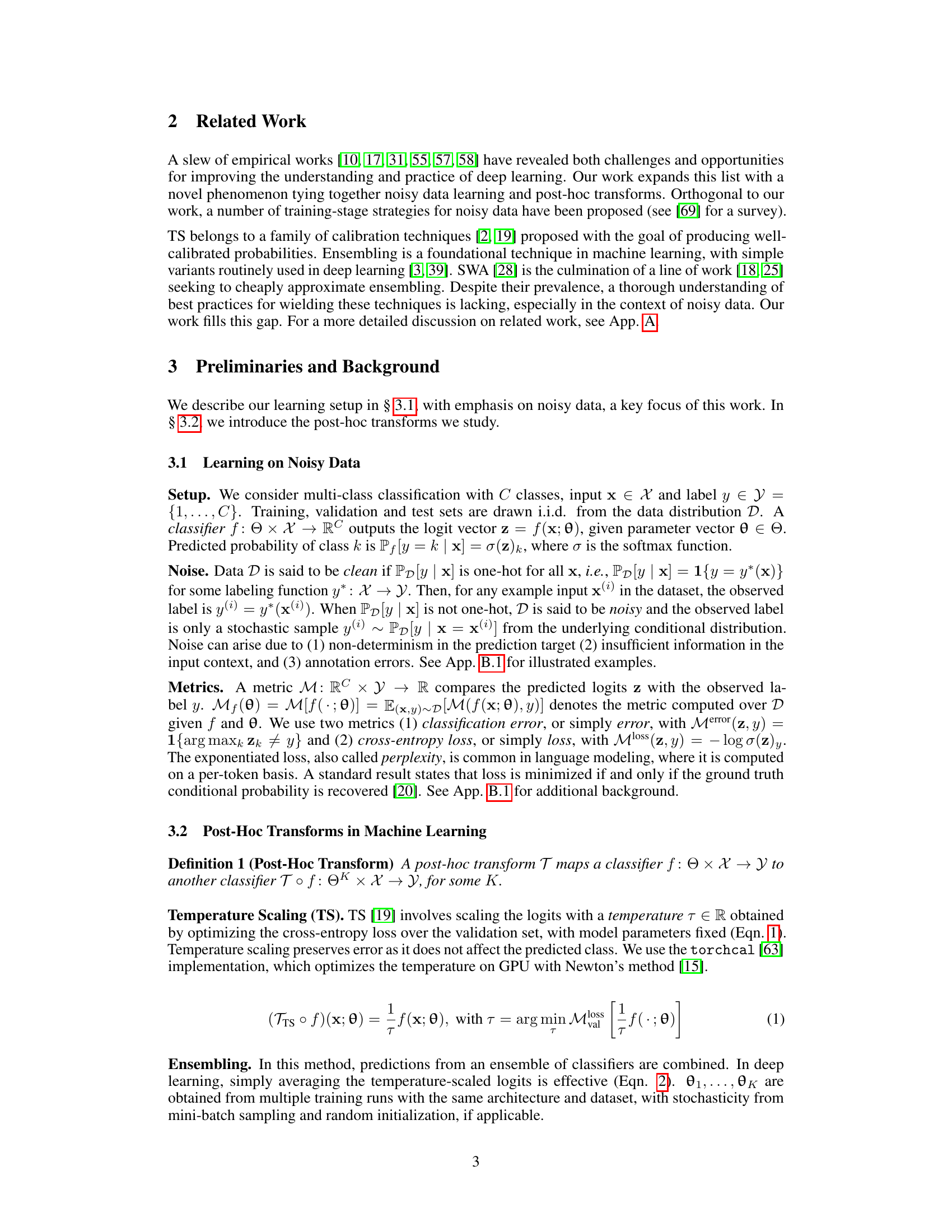
This figure compares the performance of naive and post-hoc selection methods on CIFAR-10/100-N datasets with varying noise levels using the SWA+TS transform. The results show that post-hoc selection consistently outperforms naive selection, especially in high-noise settings, often achieving more than double the improvement.
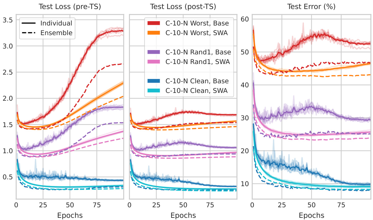
The figure shows the training curves (loss and error) for different noise levels in the CIFAR-10-N dataset. It compares the performance of base models with those that have undergone Stochastic Weight Averaging (SWA) and ensembling transformations. Key observations highlight post-hoc reversal where performance trends are reversed after applying the transformations, especially in high-noise scenarios. The impact of these transformations on overfitting and the double descent phenomenon is also demonstrated.
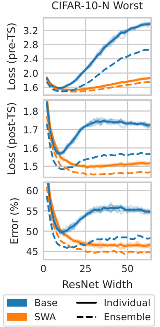
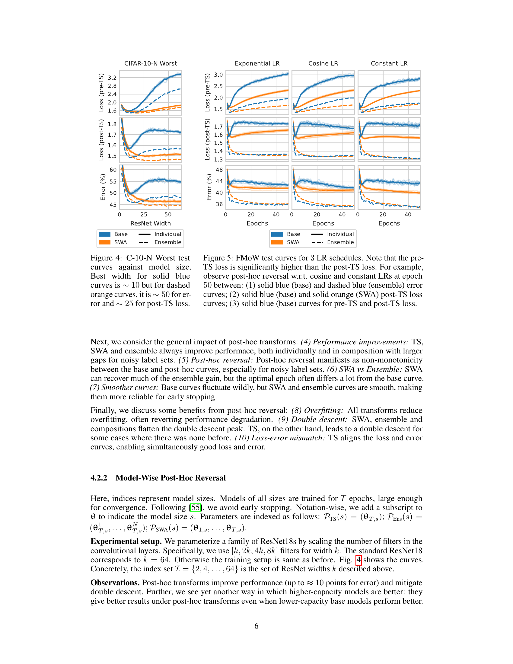
This figure shows the test curves for CIFAR-10-N Worst dataset against different ResNet widths. It demonstrates the phenomenon of post-hoc reversal with respect to model size. The base model (blue solid line) shows that a smaller ResNet width performs better early on, but after applying post-hoc transforms (SWA), a larger width is optimal. This reversal is observed for both loss and error metrics. Note the significant performance improvement due to SWA across all model sizes. The ensemble results further highlight the impact of post-hoc transforms.
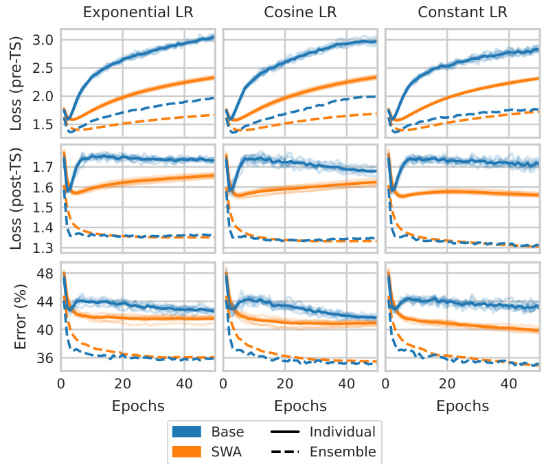
This figure shows the test curves for the FMoW dataset with three different learning rate schedules: exponential, cosine, and constant. It illustrates the phenomenon of post-hoc reversal, where performance trends differ between models before and after applying post-hoc transformations (temperature scaling, ensembling, and stochastic weight averaging). The pre-TS (before temperature scaling) loss is consistently higher than the post-TS loss for all learning rate schedules. Key observations include the reversal of performance trends between base models and models with post-hoc transformations across different epochs, highlighting the non-monotonicity between the base and post-hoc curves. This highlights how post-hoc transforms can reverse the performance trend between different models.
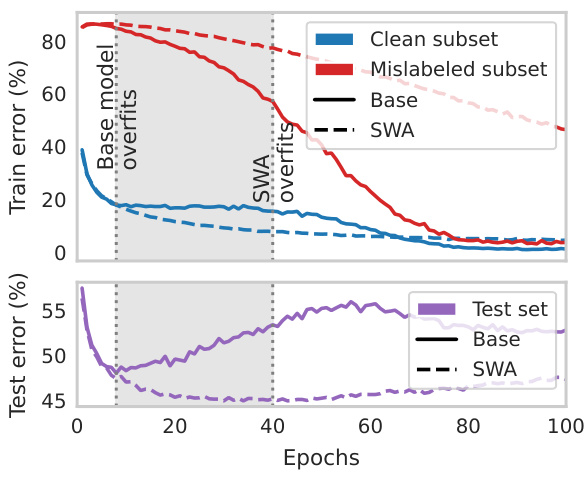
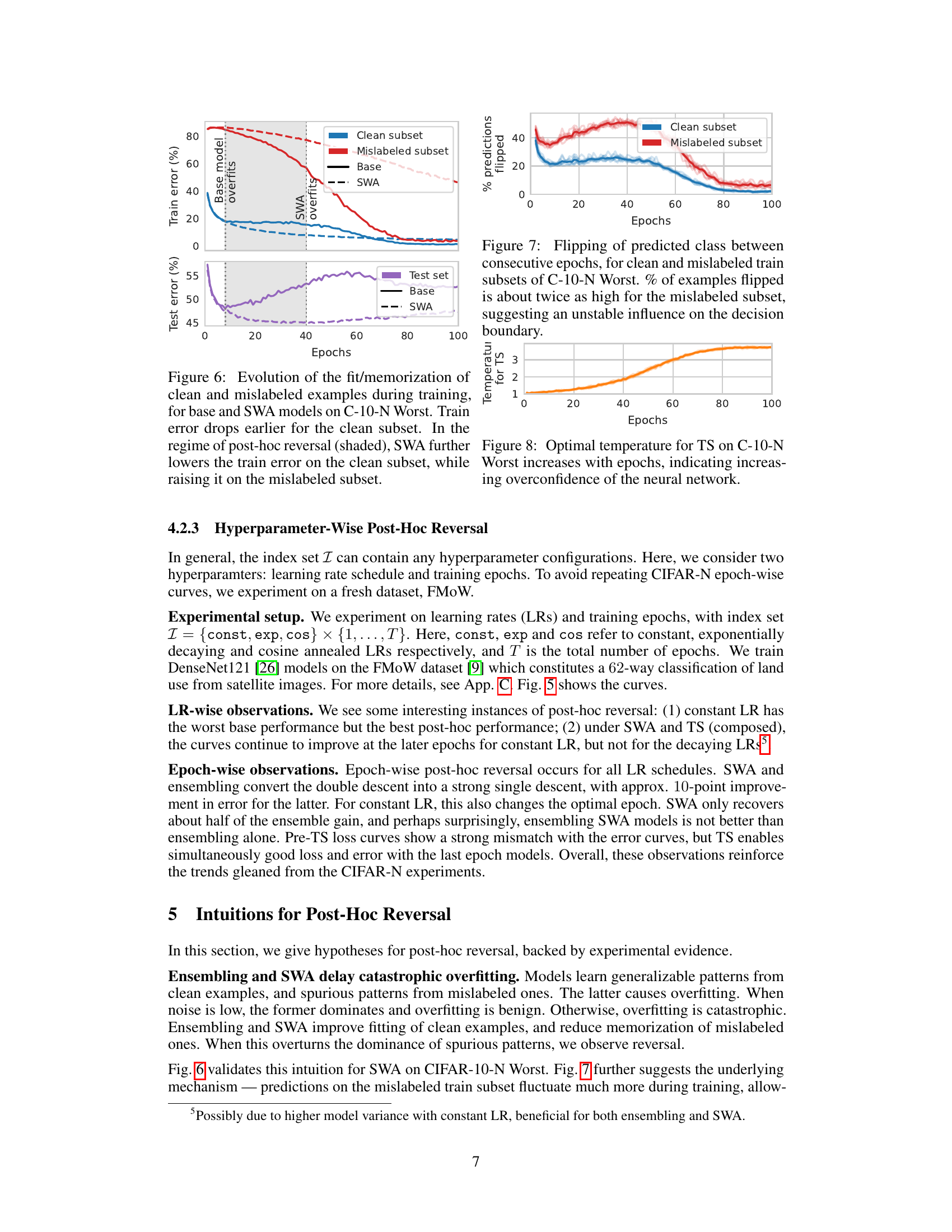
This figure shows the training and test errors for clean and mislabeled subsets of the CIFAR-10-N Worst dataset. The top plot shows the training error, illustrating how both the base model and the model using stochastic weight averaging (SWA) overfit. However, SWA overfits later than the base model. The shaded region highlights where post-hoc reversal occurs: the test error for SWA is lower than the base model, even though SWA’s training error is higher, showing that SWA helps to correct for the detrimental influence of mislabeled examples. The bottom plot shows the test error. It indicates that post-hoc reversal is happening in the epoch range between 20 and 50.

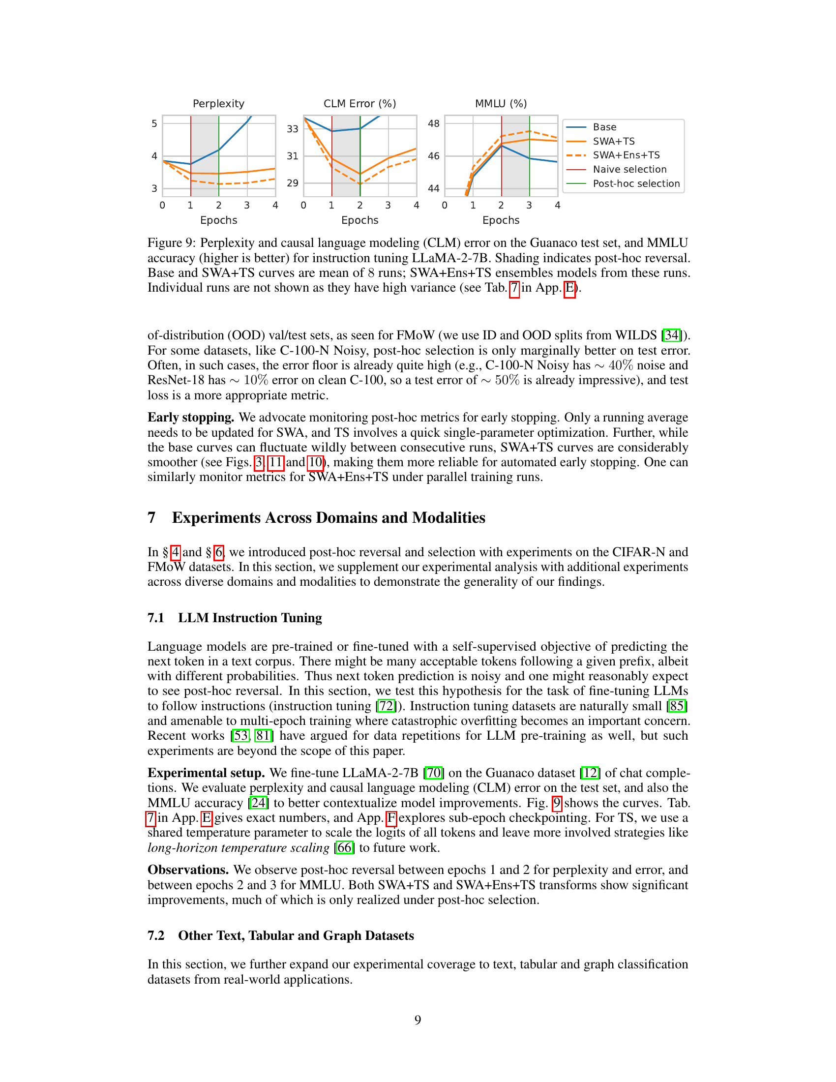
This figure shows the perplexity, causal language modeling error, and MMLU accuracy for instruction-tuning the LLaMA-2-7B model on the Guanaco dataset. It compares the performance of the base model to models using SWA+TS and SWA+Ens+TS transforms. The shaded regions highlight instances of post-hoc reversal, where performance trends change after the application of post-hoc transformations. The results suggest that post-hoc selection, which considers post-hoc metrics, outperforms the naive selection that only considers the metrics before the post-hoc transformations.
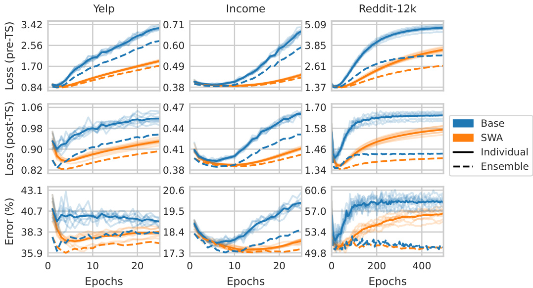
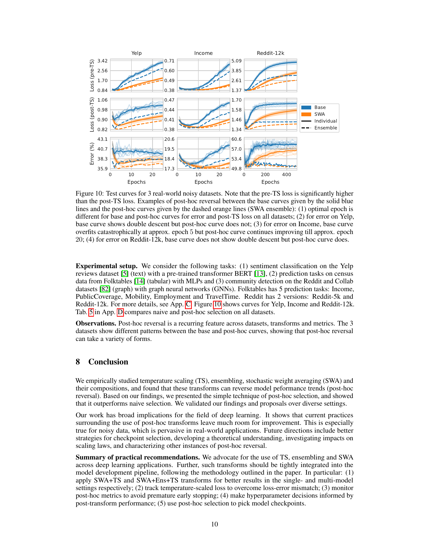
This figure shows the test loss and error curves for three real-world noisy datasets: Yelp, Income, and Reddit-12k. It demonstrates post-hoc reversal, where the performance trends (loss and error) of the base models are reversed after applying post-hoc transforms (SWA ensemble). Key observations include differing optimal epochs for base and post-hoc metrics and the impact on double descent behavior.

This figure illustrates the concept of post-hoc reversal. The naive selection method chooses a model based on its initial performance, while the post-hoc selection method incorporates post-hoc transformations (SWA, ensembling, temperature scaling) to assess performance and select a superior model based on improved metrics. The example shows a scenario where a model performs worse initially but significantly better after transformations are applied.

This figure shows the perplexity, causal language modeling error, and MMLU accuracy for instruction-tuned LLaMA-2-7B model. It compares the performance of base models with those enhanced by SWA+TS and SWA+Ens+TS post-hoc transforms across different training epochs. The shaded areas highlight instances of post-hoc reversal, where performance trends reverse after applying post-hoc transforms. Notably, the SWA+Ens+TS ensemble, which combines multiple models, demonstrates improved results overall.

This figure visualizes the decision boundaries learned by two individual models and their ensemble on a synthetic 2D spiral dataset at epochs 440 and 1000. The goal is to illustrate the phenomenon of post-hoc reversal. At epoch 440, the individual models show complex and spiky decision boundaries, especially around noisy data points. The ensemble, however, displays a smoother decision boundary. At epoch 1000, while the individual models’ decision boundaries become even more erratic, the ensemble’s boundary remains relatively consistent. This demonstrates how post-hoc transforms like ensembling can mitigate the impact of noisy data by suppressing the influence of mislabeled examples, which leads to the reversal of performance trends observed between the base models and the ensemble.
More on tables
This table compares the performance of naive model selection (selecting the best performing model based on the base metric) versus post-hoc selection (selecting the best-performing model based on the post-hoc metric after applying SWA+TS or SWA+Ens+TS transforms) on several real-world datasets. The results show that post-hoc selection often leads to better results, especially on datasets with noise in the labels.

This table details the training hyperparameters used for each dataset in the paper. It shows the model architecture, whether or not pre-training was used, the optimizer, learning rate, weight decay, learning rate schedule, number of epochs, and batch size. The datasets include image datasets (CIFAR-10/100-N, FMOW), text datasets (Yelp, Guanaco), tabular data (Folktables), and graph datasets (Collab, Reddit). Each dataset is trained with a specific set of hyperparameters optimized for that dataset.

This table shows the approximate percentage of noisy labels in different label sets of the CIFAR-N dataset. The noise is introduced by human annotators, resulting in various levels of label noise across different sets. The sets include ‘Clean’, ‘Aggre’ (aggregate of Rand1, Rand2, Rand3), ‘Rand1’, ‘Rand2’, ‘Rand3’, and ‘Worst’. The percentages represent the approximate noise level in each set, ranging from 0% (Clean) to 40% (Worst). This table is used in the paper to illustrate and define different levels of noise present in the datasets used for the experiments.
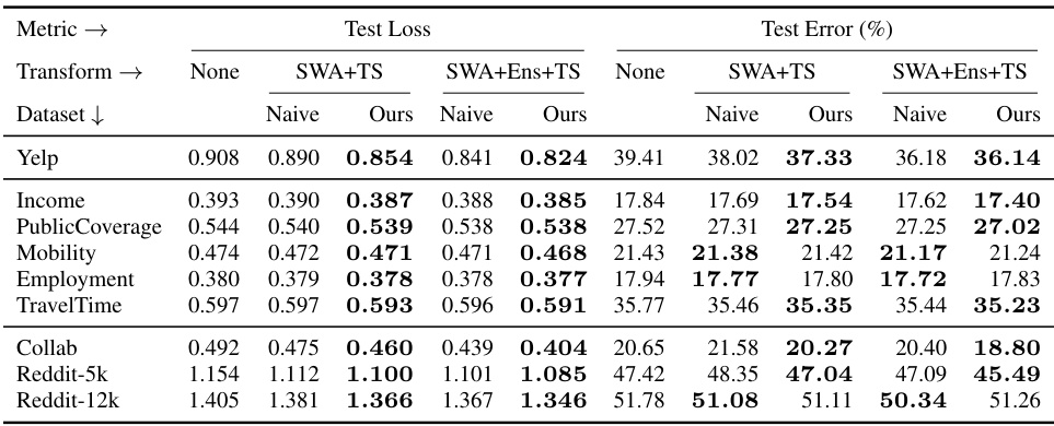
This table compares the performance of naive model selection and post-hoc selection methods using two different post-hoc transforms (SWA+TS and SWA+Ens+TS) across several real-world datasets. The naive approach selects models based on their performance before applying the post-hoc transforms, while the post-hoc approach selects models based on their performance after applying the transforms. Better results (lower test loss and error) are shown in bold, highlighting the effectiveness of post-hoc selection, particularly in improving generalization performance.
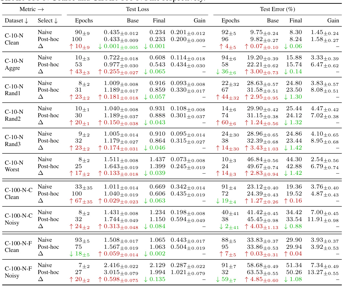
This table presents a detailed breakdown of the experimental results on CIFAR-N datasets. It compares the performance of models with no transformation (Base), with SWA+TS and SWA+Ens+TS transformations (Final), and highlights the improvement achieved by post-hoc selection compared to the naive selection method. The table includes metrics such as test loss and test error, with mean and standard deviation across multiple runs, showing results for various noise levels and dataset variations (Clean, Aggre, Rand1, Rand2, Rand3, Worst).

This table presents the detailed results for the LLM instruction tuning experiments. It compares the performance of different methods (None, SWA+TS, SWA+Ens+TS) using various metrics (Perplexity, Error, MMLU). The results are divided into those obtained using naive selection and post-hoc selection. For better readability, the values that indicate better performance are highlighted in bold. Because the base and gain calculations involve 8 separate runs, mean and standard deviation values are presented for these metrics.

This table compares the performance of naive model selection (selecting models based on their base performance before applying post-hoc transformations) against post-hoc selection (selecting models based on their performance after applying post-hoc transformations like SWA+TS and SWA+Ens+TS). The results show that post-hoc selection significantly improves performance in most noisy datasets, often more than doubling the improvement compared to not using any transformations. Standard deviations are available in appendix tables 6 and 8.
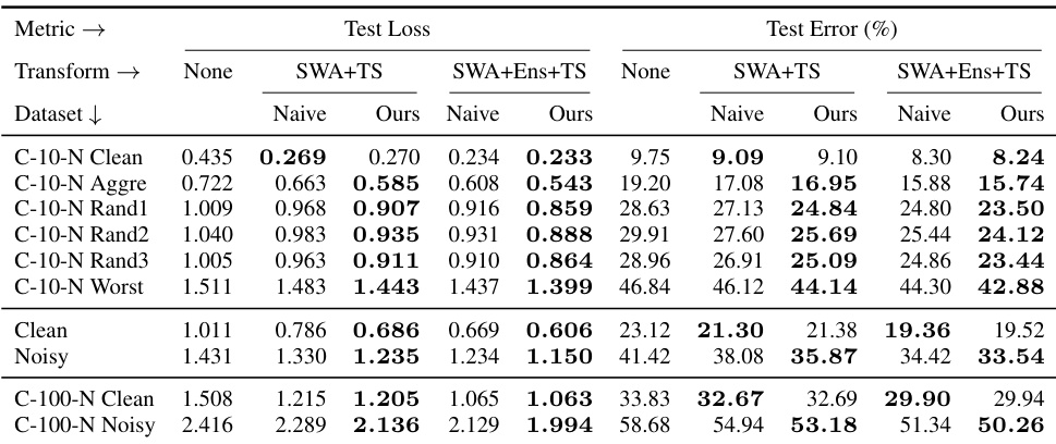
This table compares the performance of naive model selection (selecting models based on the base metrics before applying post-hoc transforms) against the proposed post-hoc selection method (selecting models based on metrics after applying post-hoc transforms). It shows test loss and test error for various datasets and transform combinations (SWA+TS and SWA+Ens+TS). The results demonstrate that post-hoc selection generally yields better results, often significantly improving upon both naive selection and the performance of models without post-hoc transformations. Standard deviations are available in supplementary tables.
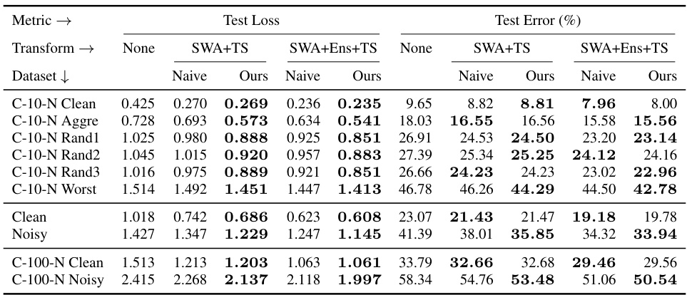
This table compares the performance of naive and post-hoc model selection methods on CIFAR-N datasets using cross-entropy loss. It shows test loss and test error for different noise levels (Clean, Aggre, Rand1, Rand2, Rand3, Worst) and for different transforms (None, SWA+TS, SWA+Ens+TS). Bold values highlight the better performance achieved with post-hoc selection.

This table compares the performance of naive model selection (selecting the best-performing model before applying post-hoc transformations) against the proposed post-hoc selection method (selecting models based on post-hoc metrics). The results demonstrate post-hoc selection’s effectiveness across various datasets and transformations (SWA+TS and SWA+Ens+TS). Post-hoc selection consistently outperforms naive selection, often resulting in more than double the improvement compared to using no post-hoc transformations. Standard deviations for all values are available in Appendix E.
Full paper#
